1. Introduction
1.1. Overview
The word cryptocurrency has become the topic of the 21st century. Not understanding cryptocurrencies is equivalent to not understanding Covid-19. The cryptocurrency was first adopted as a transaction for gaming in 2014, as suggested by [
1] that large corporations are indicating that they may legally accept it as an exchange of their goods and services.
Mukhopadhyay et al. [
2], cryptocurrency is a digital currency (digital money) in which transactions are verified, and records use a decentralised system. This decentralised system is called a peer-to-peer network and operates as cryptography, ensuring that no one controls the system, neither the government nor rich individuals. The decentralised system differs from the traditional monetary system, whereby a central bank controls a currency. To ensure security and fairness amongst the users, a well-structured complex encryption hashing algorithm constructed from the basis of blockchain technology is put in place.
Blockchain technology was not widely used until a mysterious individual who used Satoshi Nakamoto’s pseudonym created the first cryptocurrency, famously known as Bitcoin, in 2009. Due to the hidden identity of the author of Bitcoin, the cryptocurrency environment has been deemed by many as an illegal way of transacting, resulting in high volatility and the cryptocurrency crashing several times. Bitcoin may be the largest cryptocurrency by market value, but it is not the only cryptocurrency in the market.
Ethereum is the software platform enabling cryptocurrency transactions ether’; Ethereum is the second-largest cryptocurrency launched by programmer Vitalik Buterin on the 30
th of July 2015 [
3]. On the 7
th of May 2021, Ethereum had a market capitalisation of
according to [
4]. Two weeks later, the new market capitalisation is
. There is a dramatic change in price ether between the 7
th of May 2021 and 21
st of May 2021. This raises concerns for investors about whether it is a reliable asset due to its high fluctuation.
A much more informal name for machine learning is ‘the prophet method’, as it is known for its good learning algorithms to make future predictions. The development of the machine learning algorithm dates back to the 1970s by experimenting with different architectures of neurons [
5]. Machine learning is defined as the ability of a computer to learn a task without explicitly following instructions, guided by algorithms, and then be able to extract meaningful conclusive information [
6]. Machine learning may either be supervised, semi-supervised or unsupervised.
This incredible learning ability demonstrated by computers leads to the term artificial intelligence. Today, several methods have been developed that one can use to apply artificial intelligence. These include recurrent neuron networks (RNN), gradient boosting machines (GBM), generalized linear models (GLM), distributed random forests (DRF) and deep neural networks (DNN). This capstone dissertation will use RNN, GBM, GLM, DRF and DNN to predict the daily closing price of Ethereum.
Natural language processing (NLP), which was formally known as natural language understanding (NLU), is a subset of artificial intelligence (AI) used to analyse text through a set of computerised technologies and theories that are put together to imitate human-like language processing [
7]. NLP methods can process oral or written texts. For this research, only written texts will be processed by NLP methods.
We are living in an age where digital communication is thriving. Twitter has been one of the most successful and popular social media of the 21st Century. As of 2021, according to Twitter company metrics, Twitter had 221 total monetisable daily active users, with more than 500 million tweets sent per day in the fourth quarter of 2021. These users are worldwide, tweeting about different subjects, including many cryptocurrencies traded daily on crypto-exchange platforms.
Ethereum is the world’s second-largest cryptocurrency after Bitcoin, which has a much lower value, indicating that it can be used for day-to-day transactions; thus, it is important to predict its closing price due to its rapid price fluctuation. However, previous studies fail to predict Ethereum’s closing price accurately. To date, it has attracted investors and risk portfolio managers, predicting its closing price will be a good measure of risk and give investors confidence to invest in the cryptocurrency.
When trading securities such as Ethereum, investors, traders, and investment banks need to know how profitable it is to buy, hold or sell Ethereum. This study intends to forecast the daily closing price of Ethereum using machine learning algorithms RNN, GBM, GLM, DRF and DNN with the help of Ethereum tweets from Twitter.
1.2. Literature Review
Predicting the stock market volatility can be dated back to 1995 as a crucial decision-making tool. Fleming et al. [
8] aims to predict the stock market volatility. The reason behind [
8] aim is that the stock market volatility is essential for day-to-day investment decision-makers, for example, portfolio insurance. Fleming et al. [
8]’s study is structured by executing three objectives. Firstly, [
8] examines the properties of the Chicago Board Options Exchange Volatility Index (VIX) and evaluates its predictive power. Secondly, [
8] study the correlation between the volatility and the stock market returns and how well VIX predicts the stock market volatility. The VIX is modelled using the Black-Scholes framework using the implied volatility of eight Chicago Board Options Exchange options. The results detail that VIX strongly correlates with the expected stock market returns, indicating that it is a good measure.
Other variables other than price returns have been used to forecast price volatility. Jain and Jiang [
9] aim to predict future price volatility using the limit order book (LOB) from the Shanghai Stock Exchange (SHSE). The data is obtained from SHSE from January 2009 to December 2009. A LOB slope was constructed that will be used in the prediction process. It is concluded that LOB efficiently predicts price volatility with the limitations of poor performance during major market-wide movements. The underlying factor of efficiently predicting price volatility is the high correlation between buy orders and future price volatility.
If the security is big enough for market capitalisation, its price might impact the stock market volatility. Tang et al. [
10] investigated the oil future price predictability power towards the United States (US) market volatility. The use of autoregressive conditional heteroskedasticity methodology is applied to construct models. Data is obtained from the Thomson Reuters Tick History Database from January 2007 to April 2017. It is concluded that oil future price predictability significantly predicts the US stock market.
Generalised autoregressive conditional heteroskedasticity (GARCH) models are less computationally expensive than ANN (artificial neural network) models; however, the rapid development of computers allows us to compare the best model between the two in predicting historical volatility. [
11] investigates the best approach for forecasting currency exchange rate volatility. The data consist of daily exchange rates from January 2010 to December 2013 collected from the federal economic database. The dataset is split into 80% for the training set and 20% for the testing set. The three models compared to each other are the GARCH, exponential-GRACH, and ANN. The ANN model outperforms the other models in predicting historical volatility because it produces the least mean square error.
When assessing a risk portfolio, one needs accurate technical measures. Combining models known to be great volatility predictors may be very fruitful. [
12] investigated the effect of combining RNN with LSTM and multiple GARCH models to forecast volatility. The data is collected from the KOSPI 200 index returns between January 2001 and September 2011. The models used in the combination technique are exponential weighted moving average (EWMA), EGARCH and RNN with LSTM. The combined RNN model with LSTM and three GARCH-type models produced the best predictions with a mean absolute error of 0.0107.
The use of RNN predictive power works well with time-series data. Anbazhagan and Kumarappan [
13] proposed predicting deregulated electricity market price for the next day in Spain. The architecture of RNN is Elamn Network, which proves to be very robust. The Elman network is compared to other models such as the autoregressive integrated moving average (ARIMA), weighted nearest neighbours, wavelet ARIMA, neural networks with wavelet transform and wavelet-ARIMA radial basis function neural networks. The results conclude that the proposed RNN with Elam Network is the most efficient model.
Derbentsev et al. [
14] focused on predicting three cryptocurrencies using Random Forests (RF) and Stochastic Gradient Boosting Machine (SGBM). The three cryptocurrencies are Bitcoin (BTC), Ethereum (ETH) and Ripple (XRP). The dataset is their historical daily close prices. To check the effectiveness of these models, an out-of-sample forecast was made for the selected time series using the one-step ahead technique. For the three cryptocurrencies (BTC, ETH, and XRP), the out-of-sample accuracy of the short-term prediction daily close prices derived by the SGBM and RF fell between 0.92 and 2.61 in terms of Mean Absolute Percentage Error (MAPE). The outcomes confirm that the ML ensembles approach may be applied to forecast cryptocurrency prices.
Poongodi et al. [
15] proposed using a time series made up of the closing values of the cryptocurrency Ether every day, two machine learning techniques—linear regression (LR) and support vector machine (SVM)— to predict daily closing prices. Filters with varying weight coefficients are employed to anticipate the price of ether cryptocurrency over a range of window lengths. Cross-validation is a technique used in the training phase to build a high-performance model that is not dependent on the dataset. The results showed that the SVM method has a higher accuracy (96.06%) than the LR method (85.46%).
Deep learning models are known to be good predicting models; recently, researchers have been investigating if they are better when stacked together. [
16] proposed ensemble models evaluated as combinations of long short-term memory (LSTM), Bi-directional LSTM and convolutional layers. The ensemble models were tested for regression (predicting the next hour’s cryptocurrency price) and classification (predicting whether the price of a cryptocurrency will rise or fall in relation to the current hour). Empirical results from the study showed that deep and ensemble learning can effectively support one another in creating robust, steady, and dependable forecasting models.
Henrique et al. [
17] investigated the relationship between social media posts and the volatility price movement of cryptocurrency. This was achieved by analysing the social media posts of a Chinese platform, Sina-Weibo, Sina-Weibo, WeChat, and QQ groups. Sina-Weibo can produce approximately 24000 accompanied by 70000 comments and tweets about cryptocurrency in just eight days. A sentiment dictionary is constructed to categorise three distinct moods from the tweet. These are bag holders, new highs, and abandoned ships. Combining these social media sentiments with an RNN with LSTM fueled by historical cryptocurrency price is more efficient in predicting the volatility price movement than the based ARIMA model by 18.5% accuracy.
Vadivukarassi et al. [
18] investigated the polarity of tweets from Twitter as either positive or negative. Luo et al. [
19] extracted the tweets from Twitter using Twitter API. A Chi-Square test and a naïve Bayes classifier are used for training and testing the model for selecting the best features to evaluate sentimental polarity using Python. Different features of s 10,100,1000,10000 were applied respectively. It was concluded that as the number of features increases, the accuracy of the selected feature also increases.
Luo et al. [
19] presented an NLP framework that uses sentiment analysis to analyse the opinions of Twitter users on Human papillomavirus (HPV) vaccination over ten years from 2008 to 2017. Luo et al. [
19] used sentiment analysis and AI, amongst other methods, on the phrase ‘
associationmining’ search through Twitter. The results showed that from 2008 to 2011 and 2015 to 2016. The top negative words were safety concerns, deaths, adverse/side effects, injuries and scandal, while the top positive words were cervical screens, prevents, vaccination campaigns and cervical cancers. The result from the sentiment analysis helped public health researchers gain a better understanding of the influence of social media on HPV vaccination attitudes and also develop strategies that will deal with misinformation.
The use of machine learning models and the application of NLP with naive Bayes classifying tweets into positive or negative news has been discussed in detail in the above literature review. This research seeks to study the effect of adding tweets as an additional variable in predicting the closing price of cryptocurrency.
1.3. Research Highlights and Contributions
The main contribution of this study is to carry out a comparative study of the predictive capabilities of some machine and deep learning algorithms with a stacking ensemble modelling framework of ETH closing prices for the next two days using historical Ethereum prices and Ethereum tweets. The rest of the paper is organised as follows. A discussion of the modelling closing price of Ethereum using the RNN, Stacked RNN, GBM, GLM, DRF and DNN, Stacked GBM, GLM, DRF and DNN (GGDD) is given in
Section 2. Empirical results are presented in
Section 3 while
Section 4 presents a discussion of the performance of the models.
Section 5 concludes.
2. Methods
2.1. Natural Language Processing Method
Naive Bayes is the NLP method for text (tweet) classification into good or bad news. The classified tweet will be treated as an additional explanatory variable coded 0 and 1 for good and bad news, respectively. The naive Bayes model is part of a group of generative models in NLP. The Naive Bayes model is given in equation (
1) [
20].
where
k is the class containing 1 for good news and 0 for bad news, and
) is the feature vector. As input is embedded into the NLP model, it will go through the function TextBlob, a classifying technique for tweets into either good/positive news or bad/negative news. The TextBlob will compute the subjectivity and polarity of the tweets. If the polarity of the tweet is positive, it will be considered good news, and if it is negative, it will be considered bad news.
2.2. Recurrent Neural Network with LSTM
RNN is despised for having a gradient vanishing problem, which results in poor results. Through this challenge, a modified version of RNN with long short-term memory (LSTM) was developed [
21]. RNN with LSTM is an advanced version of RNN that remembers past data in memory using three gates in each neuron in the hidden layer. The three gates are the input gate, forget gate and output gate. The input gate modifies the memory; the forget gate decides what details to discard from the block, and the output gate combines the values from the input gate and the forget gate.
RNN algorithm is implemented by initialising weights, forward propagation and backward propagations. After the output has been calculated from the forward propagation during training, the error between the predicted and actual values is used to adjust weights using mini-batch gradient descent. Adjusting these weights from the output layer to the first layer is called Backward propagation. Most RNNs primarily use the following activation functions sigmoid, hyperbolic tangent (tanh) and Rectified linear unit (ReLu). These activation functions help prevent the gradient from exploding and vanishing.
Equation (
2) defines the sigmoid activation.
The tanh function is defined by equation (
3).
The ReLu function is given in equation (
4).
2.3. Gradient Boosting Machine
The second methodology used is the Gradient Boosting Machine (GBM), a recommended algorithm, which [
22] proposed. The GBM algorithm is a forward learning ensemble method driven by the principle that more accurate approximations can yield better prediction outcomes. Regression trees are progressively constructed on all of the dataset’s characteristics by H2O’s GBM in a completely distributed manner; each tree is constructed in parallel. Gradient boosting machines have demonstrated notable effectiveness in a variety of real-world applications. They can be easily tailored to meet specific application requirements and establish a connection with the statistical framework, such as learning various loss functions [30]. In order to produce a response variable estimate that is more precise, the GBM learning process fits new models one after the other. This technique’s main concept is to build new base-learners with the highest possible correlation with the loss function’s negative gradient [30].
Because of their great adaptability, the GBMs may be tailored to almost any specific data-driven task. It adds great flexibility to the model design, so selecting the best loss function becomes a trial-and-error process. Given a dataset that has a response variable y and a set of explanatory variables
with a training sample
of known
[31]. The GBM general formula to estimate the response variable is given in equation (
5).
where function
,is a simple parameterized function of the input variables x, characterized by parameters
.
2.4. Generalized Linear Model
The third methodology will be used is the Generalized Linear Model (GLM). [
23] describes GLM as a family of models consisting of Gaussian regression, Poisson regression, Binomial regression (classification), Fractional binomial regression, Quasibinomial regression, Multinomial classification, Gamma regression, Ordinal regression, Negative Binomial regression and Tweedie distribution. Given the nature of our data, which is in an integer form, the evaluation model used is Gaussian regression.
According to [
23], the dependence between a response vector (y) and a covariates vector (x) is modelled by Gaussian as a linear function given by the following function:
where
,
and
is the error coefficient.
2.5. Distributed Random Forest
The fourth methodology that will be used is the Distributed Random Forest (DRF). Instead of producing a single classification or regression tree, [
24] states that DRF creates a forest of them. Weak learners are based on a subset of rows and columns comprised of each tree. The variance will decrease with more trees. Whether predicting for a class or a numerical value, classification and regression both use the average prediction across all of their trees to arrive at a final prediction.
Cevid et al. [32] suggested a forest design for multivariate responses based on their joint conditional distribution, independent of the estimation target and the data model. If we let
be a multivariate random variable representing the data of interest, but whose joint distribution is heterogeneous and depends on some subset of a potentially large number of covariates
. An estimate of the conditional distribution will give a certain target object
:
where
is an arbitrary point in
.
2.6. Deep Neutral Networks
The fifth methodology will be used is the Deep Neutral Networks (DNN). [
25] illustrates how a multi-layer feedforward artificial neural network trained by back-propagation stochastic gradient descent is the foundation for deep learning. Numerous hidden layers of neurons with maxout, rectifier, and tanh activation functions may be present in the network. High prediction accuracy is made possible by sophisticated features like adaptive learning rate, rate annealing, momentum training, dropout, L1 or L2 regularization, checkpointing, and grid search.
Since the deep learning model of the neural network was compiled using
. The methodology below primarily focuses on the feedforward architecture used by
. This model uses a similar architecture to the RNN, which has a weighted combination of aggregated input signals given by [32]:
having an output signal
transmitted by the connected neuron. Unlike the RNN described in sub
Section 2.2, the Deep Neutral Network uses the LSTM extension. However, it uses the same activation functions illustrated in equations (
2) to (
4).
2.7. Stacked Ensemble
The seventh methodology used is the Stacked Ensemble for GBM, GLM, DRF and DNN (ESGGDD). According to [
26], the Stacked Ensemble method is a supervised ensemble machine learning algorithm that uses a technique known as stacking to determine the best configuration of a set of prediction algorithms. This paper stacks GBM, GLM, DRF and DNN to produce a stacked GMM GLM DRF DNN (GGDD model). Another stacked model will combine three RNN models trained at different train test split ratios.
The stack ensemble method used here is from the to find the optimal combination from several predictions. stacked ensemble algorithm is included in the system algorithms here [34].
2.8. Model Forecast Accuracy
The best-performing models will be selected under the following criteria:
2.8.1. Root Mean Square Error
Root mean squared error (RMSE) is the square root of the second sample moment of the differences between predicted and observed values or the quadratic mean of these differences, [
27]. Its formula is given by:
where
is the predicted value,
is the actual value
n is the total number of observations.
2.8.2. Mean Square Error
Mean squared error (MSE) measures residuals squared between the expected and actual observations, [
28]. Its formula is given by:
where
is the predicted value,
is the actual value and
n is the total number of observations.
2.8.3. Mean Absolute Error
Mean absolute error (MAE) measures absolute errors between the expected and actual observations, [
29]. Its formula is given by:
where
is the predicted value,
is the actual value and
n is the total number of observations.
3. Empirical Results and Discussion
3.1. Exploratory Data Analysis
The dataset of daily observations of the closing price in Ethereum’s United States Dollar (USD) currency has been obtained from a reliable open source called Coindesk. It is dated from the 1st of January 2022 to the 6th of December 2022.
The primary data used is quantitative. The closing price of Ethereum will be used in calculating lag1 and lag2. The tweets will be extracted using the search of #Ethereum on Twitter. Preprocessing the data includes:
Evaluating the lag1 and lag2 from the daily closing price, which will be used as two covariates.
Evaluating the noltrend from the daily closing price will be used as one of the covariates.
Extracting a monthtype variable from each observation date, which is to be used as one of the covariates.
Extracting a type variable from the date of each observation, which is to be used as one of the covariates.
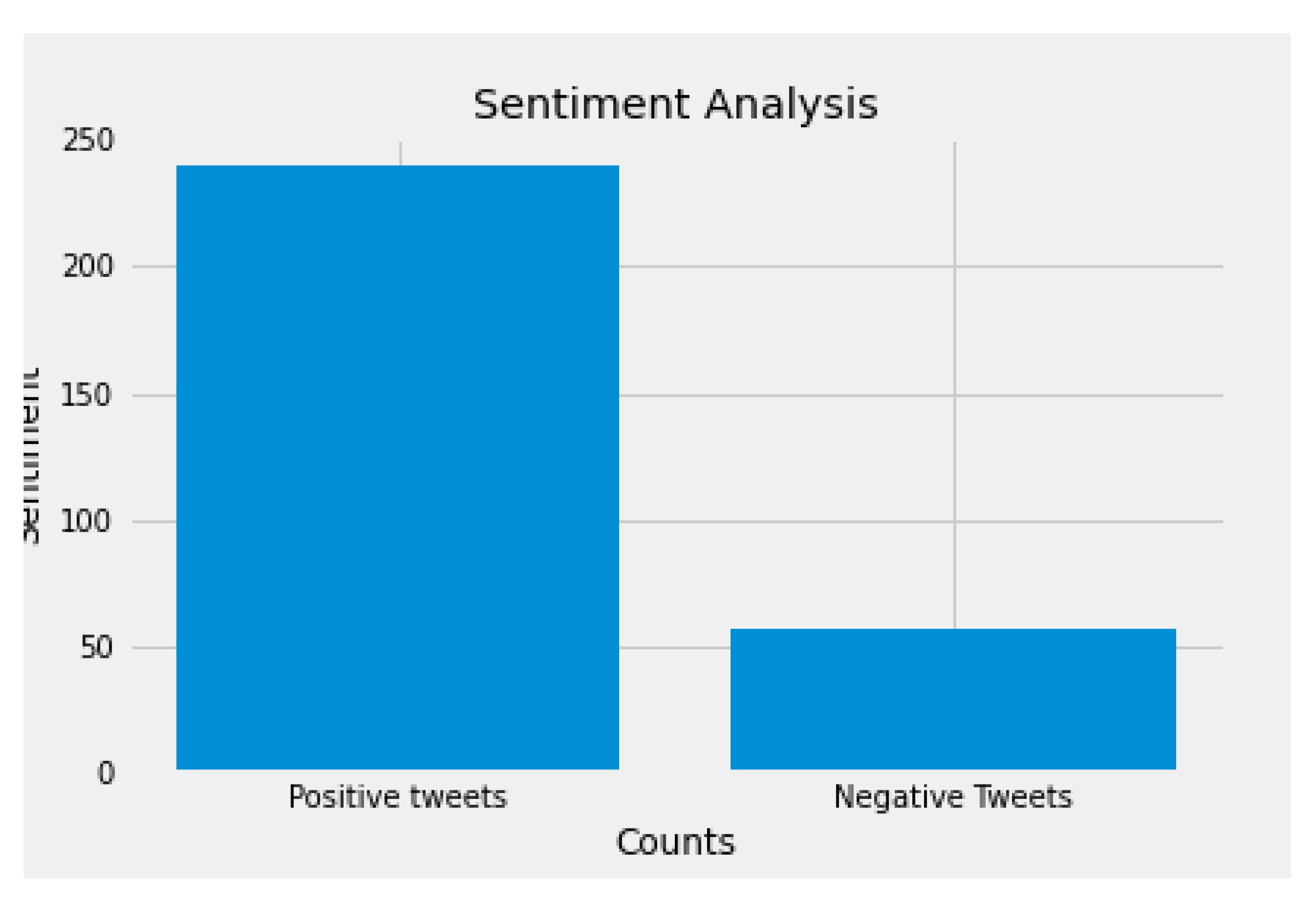
Computing positive and negative sentiments from tweets using a naive Bayes classifier.
Hot-coding positive news as 1 and bad news as 0.
The response variable is the daily closing price of Ethereum that undergoes scaling transformation to reduce the range between maximum and minimum closing price. The data will be split into three train and test splits; 80:20, 90:10 and 95:5. The variables in the dataset are described as follows:
Ethereum Closing Price (ETH_CP): this is the daily closing price of Ethereum.
Lag 1 (lag 1): this is the computed first lag of each closing price of Ethereum.
Lag 2 (lag 2): this is the computed second lag of each closing price of Ethereum.
Daytype (lag 2): this is the computed day from each date of each closing price of Ethereum.
Monthtype (lag 2): this is the computed month from each date of each closing price of Ethereum.
Noltrend 2 (lag 2): this is Ethereum’s computed smooth spine of the closing price.
Tbc (lag 2): this is the computed tweet polarity of each closing price of Ethereum.
Table 1 shows summary statistics of the overall data. It displays the minimum value (min), first quartile (Q1), mean, median, third quartile (Q3), maximum value (Max), Skewness and Kurtosis. There are 294 observations of each variable. The ETH_CP has a minimum of
and a maximum of
. The range between the minimum and maximum
is more than
$2000. Hence, the scaling transformation has reduced the range, making it easier to compute the predictions. The ETH_CP has a skewness of 0.244, and the kurtosis of
reflects a platykurtic curve that has lighter tails than its normal distribution.
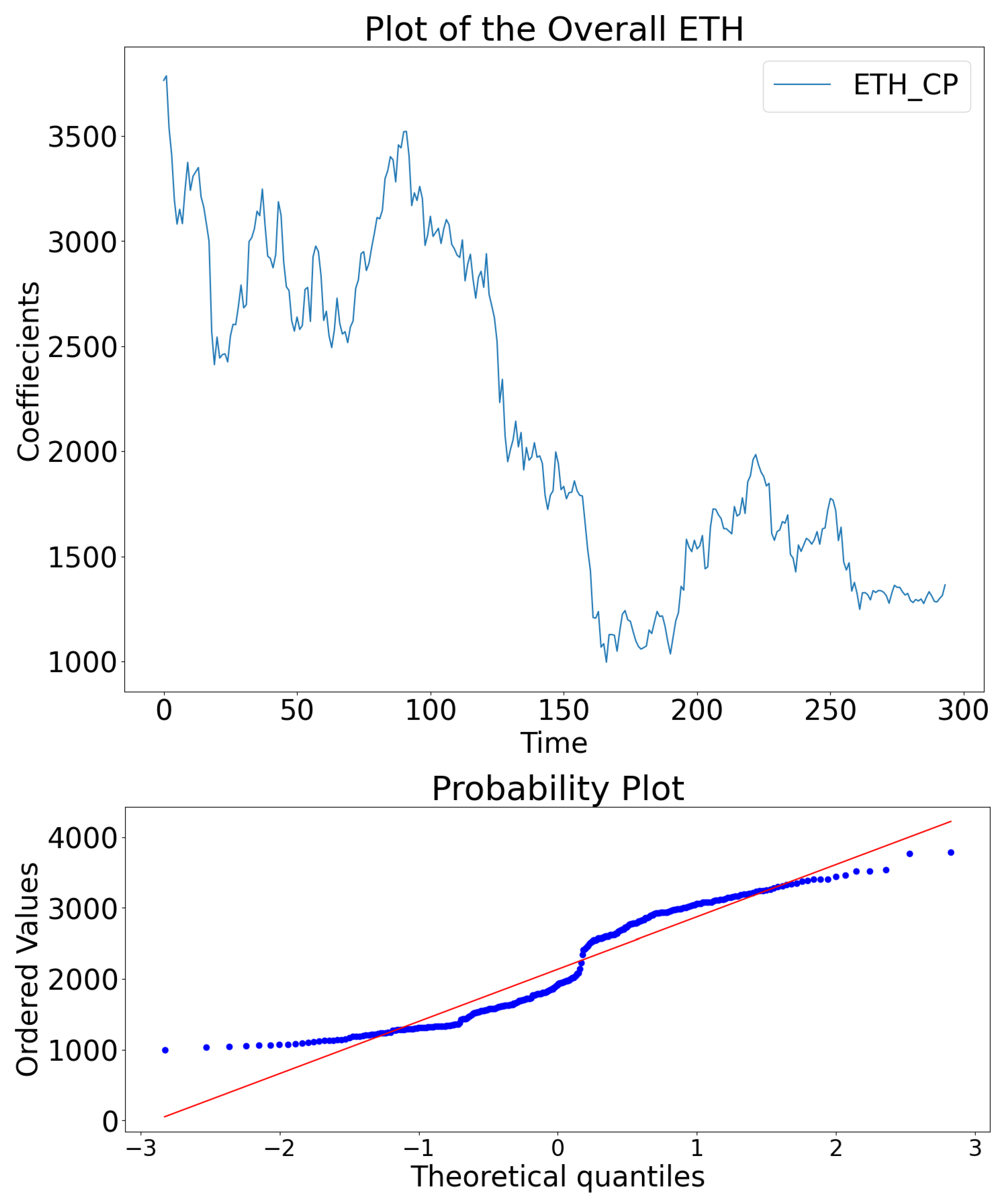
Figure 1 top panel displays
, showing a better visual display of closing prices of Ethereum over the months. The quantile-quantile plot illustrated in
Figure 1, bottom panel indicates that
is not a typical normal distribution since it has heavy outliers in the left and right tails. Furthermore, an evaluation of the chi-square normality test at
alpha level of significance with the null hypothesis of
is a normal distribution and alternative hypothesis that
is not a normal distribution. The test produced a p-value less than
of
, indicating that
does not display a normal distribution after rejecting the null hypothesis.
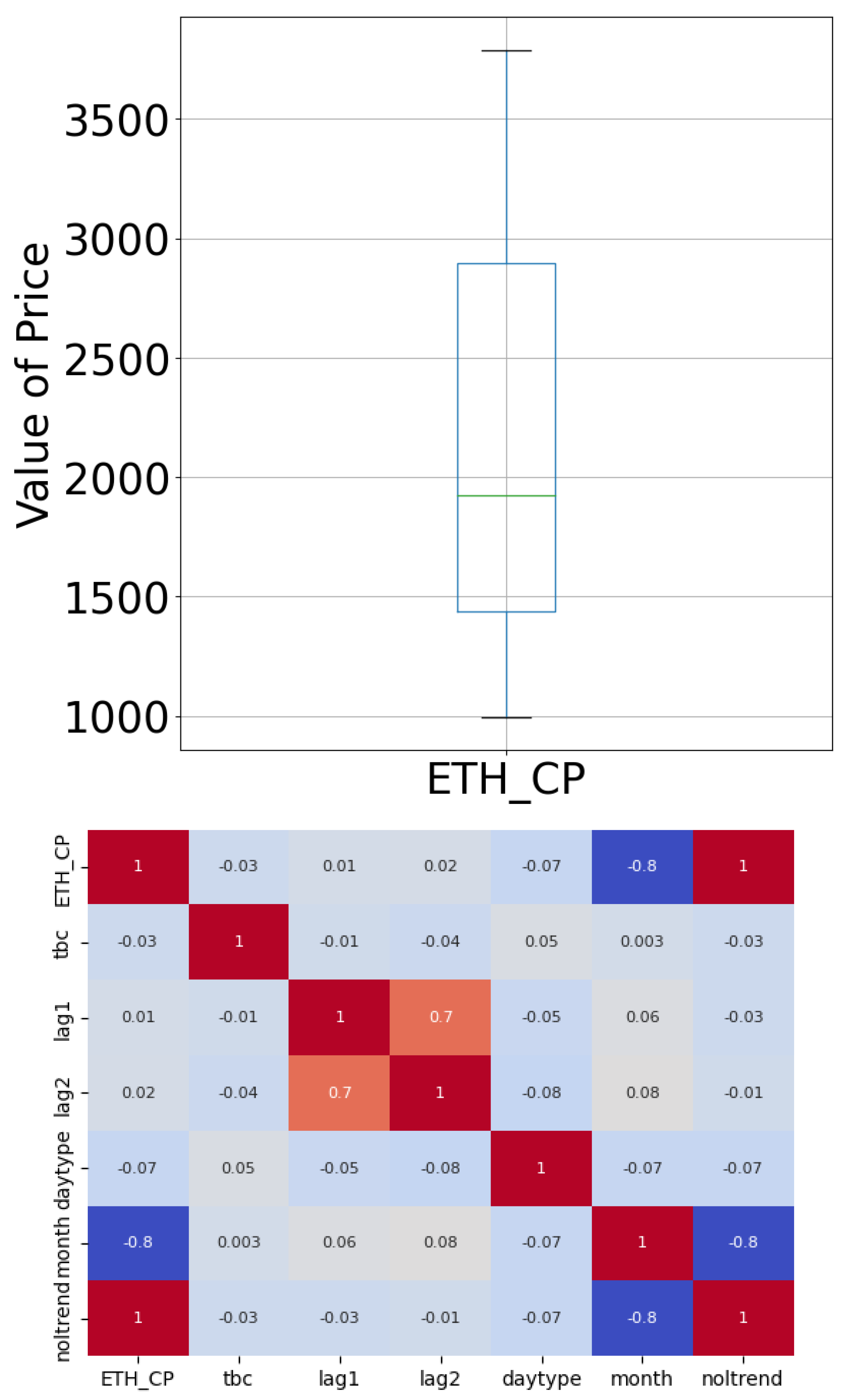
The box and whiskers plot in
Figure 2 top panel represents the density distribution and the outliers.
Figure 2 top panel displays a non-asymmetric distribution, which does not represent a normal distribution with many outliers on its tails.
Figure 2 bottom panel evaluates the correlation of the elements in the dataset. Noltrend and monthtype are the only covariates with a good correlation with
, meaning the variables are highly related to the response variable; the rest have little correlation with
.
A total of 788 tweets were extracted from Twitter from the 1st of January 2022 to the 06th of December 2022 using the following query on Twitter APIs: “
" This query assists in reducing Ethereum tweets noise as it makes sure that the tweets do not contain certain keywords that are not inline with Ethereum. The tweets were then subjected to data cleaning, which includes removing mentions, unwanted symbols, retweets and hyperlinks, as shown in
Table 2.
Table 2 further shows that by using the Textblob function, subjectivity and polarity were computed to indicate whether the tweet is good or bad news. If the polarity of the tweet is less than one, then it is bad news. If it is greater than one, it is considered good news. Since there is more than one tweet that can be good or bad, the tweets are further aggregated into one category daily. For example, if on the 1st of January, there are three tweets of bad news and one tweet of good news, the four tweets will be aggregated, and the 1st of January will be assigned 0 as
, meaning that the outcome of the 1st of January is negative.
Figure 3.
Partial Extracted tweets of #Ethereum.
Figure 3.
Partial Extracted tweets of #Ethereum.
3.2. Results
Table 3 summarises the accuracy measures of the seven comparative machine learning models evaluated at three train test ratios, i.e. 80:20, 90:10 and 95:5. All models had the same subset of training and testing data. The models were evaluated using three accuracy measures, i.e. MAE, MSE and RMSE. GLM is the model that had the lowest MAE of 21.31 when evaluated at a 95:5 train test ratio. An MAE of 21.31 means that on average days, the GLM predictions will be off the actual value by an error of
$21.31. This means that after creating a lower and upper bound of
$21.31 when forecasting the closing price of Ethereum, and it happens that it is sufficient when compared to the actual value, the investor can estimate their profitability when trading.
Furthermore, GLM also had the lowest MSE and RMSE when evaluated at a 95:5 train test ratio. According to MAE, the second-best model that performs well after GLM is the RNN, which produced an MAE of 29.81. This hierarchy of performance was followed by Stacked GGDD, GBM, Stacked RNN and DRF, respectively, up until we got to the least performing model according to MAE the DNN, which produced an MAE of 81.26 when evaluated at 95:5 train test ratio.
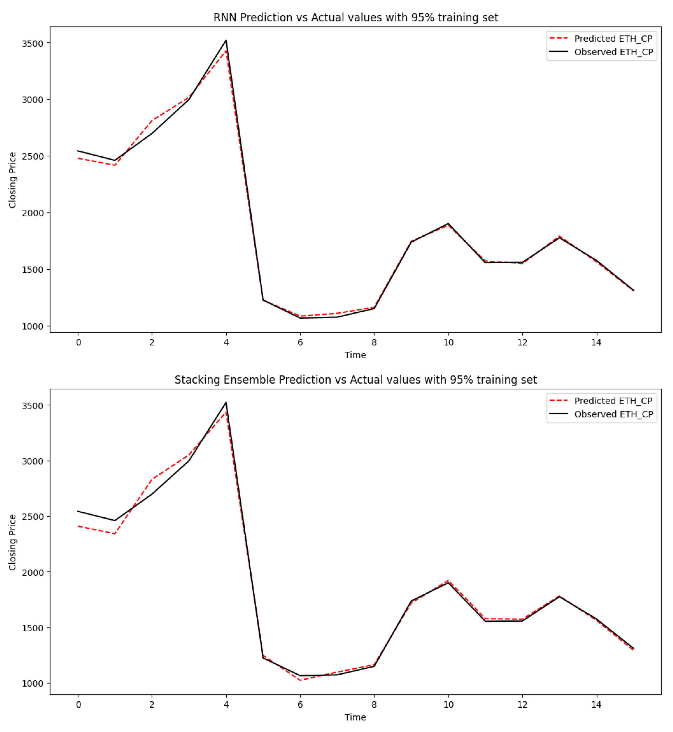
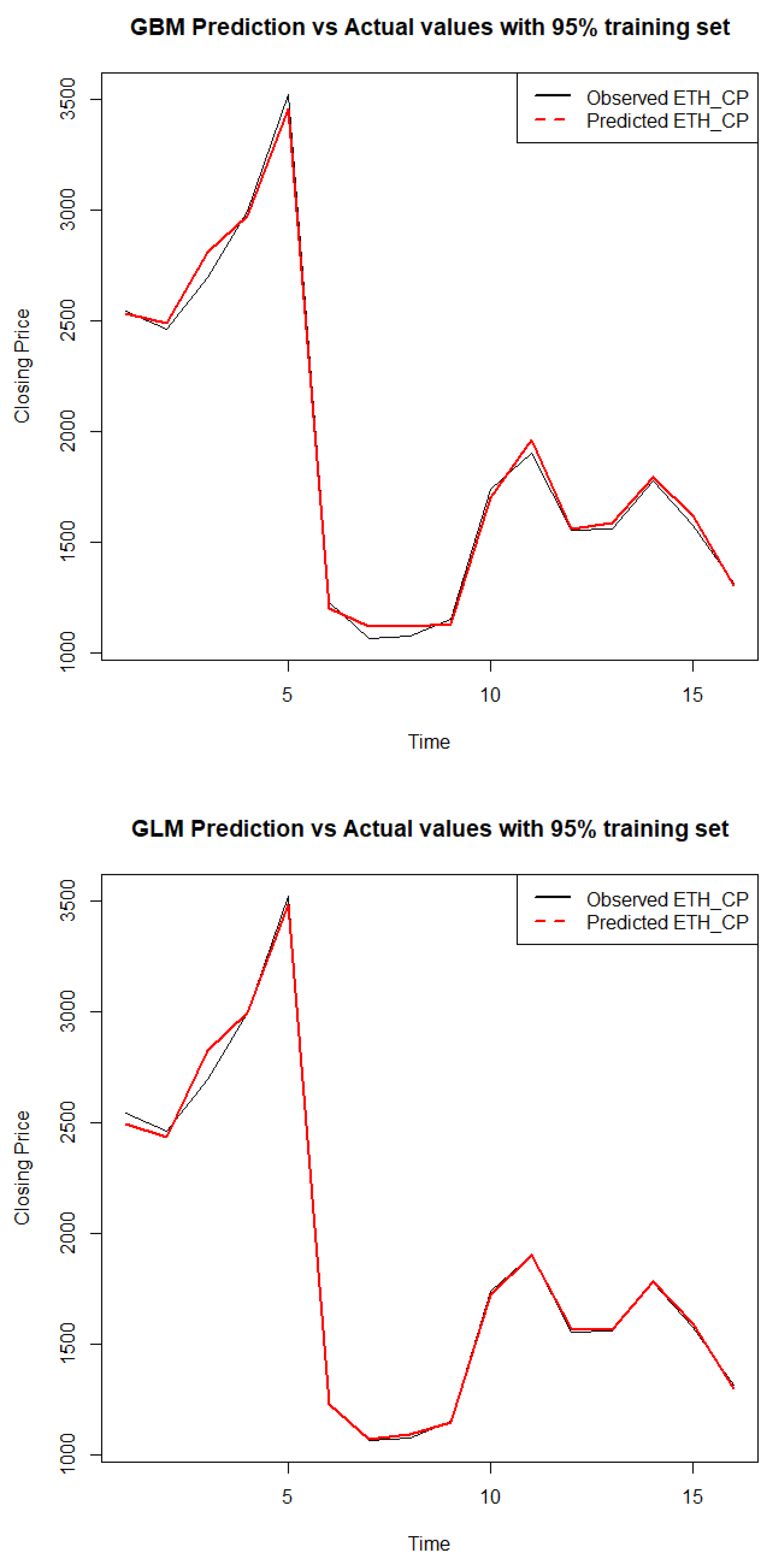
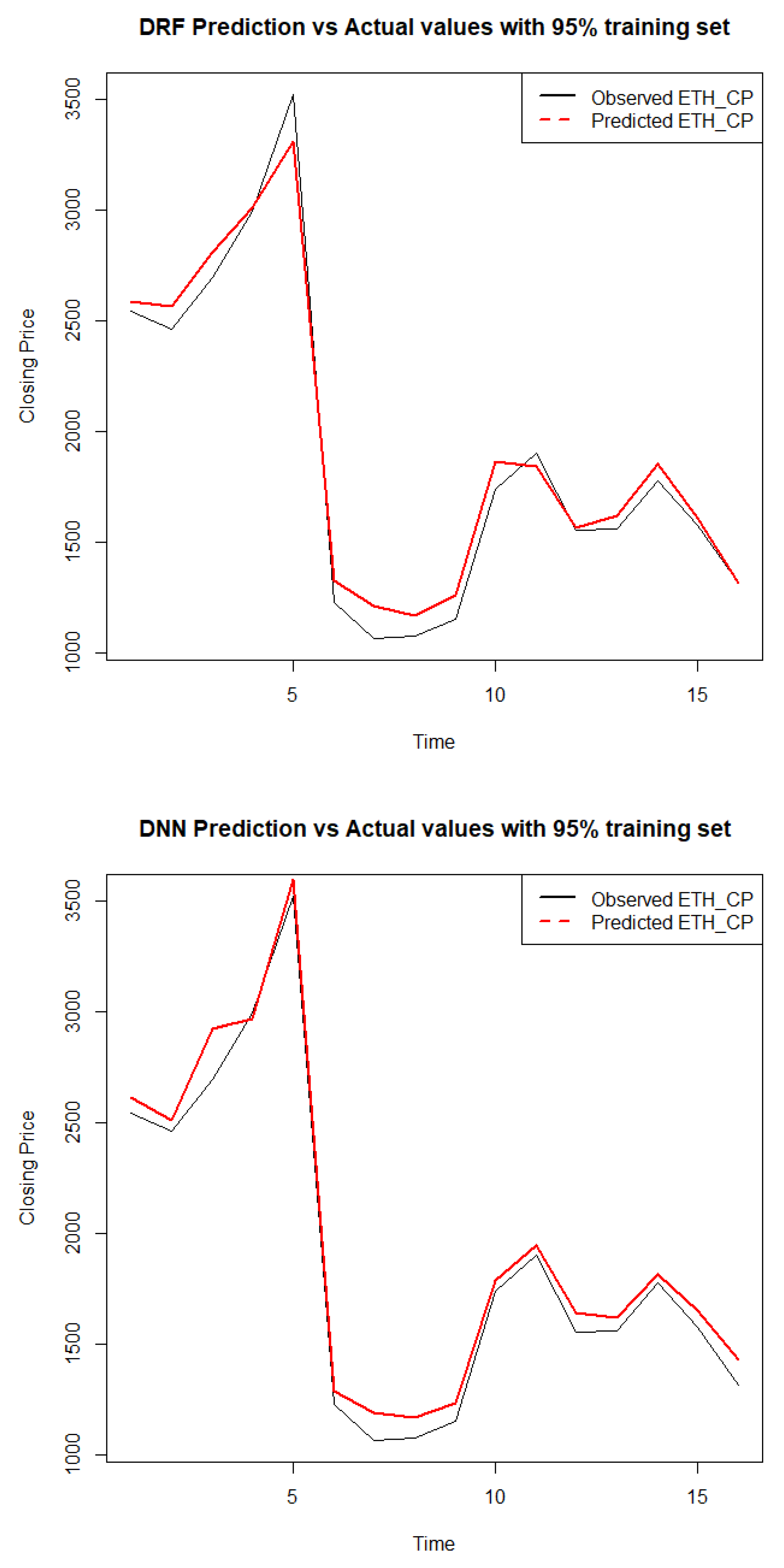
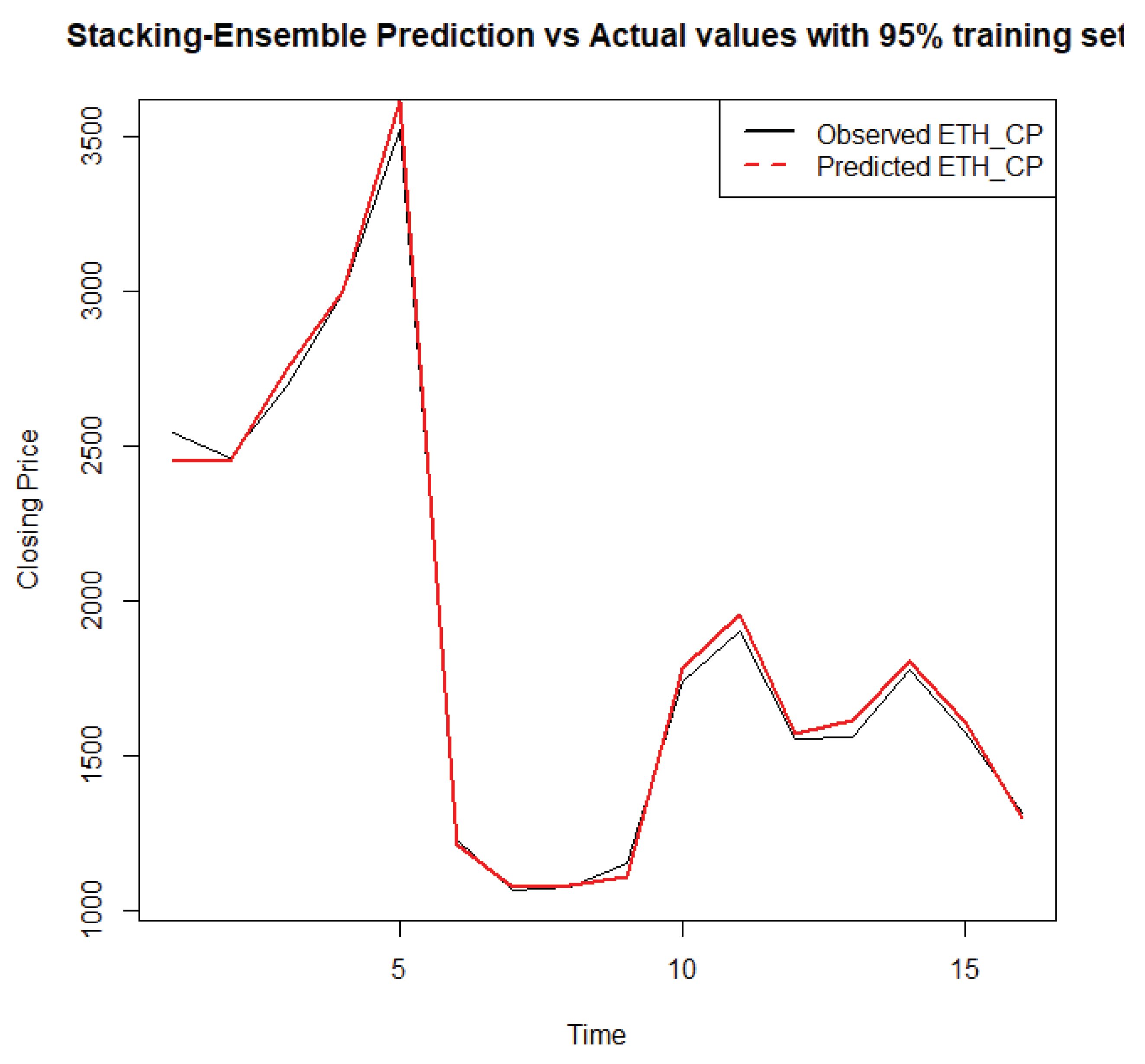
Figure 4,
Figure 5,
Figure 6 and
Figure 7 display the forecasted closing price of Ethereum against its actual closing price of all the models when evaluated at a 95:5 train test ratio. The red lines show the predicted values, whereas the black lines show the observed values. It is evident from
Figure 5b, which displays the GLM model, that the predicted and observed values are very close to each other, whereas, in
Figure 6b, which displays the DNN model, it is evident that the observed and actual values are not so close to each other as compared to
Figure 5b.
4. Discussion
The study focussed on the complexities of predicting Ethereum’s daily closing price, a cryptocurrency known for its volatile nature. With the widespread acceptance of cryptocurrencies as an alternative payment and currency exchange mode, the financial world has seen a surge in interest from academics, economists, investors, traders, and investment banks. However, accurately forecasting cryptocurrency prices remains a formidable challenge due to their rapid fluctuations.
The study uses deep learning algorithms within a stacking ensemble modelling framework to tackle this prediction task. This approach integrates various models to harness their collective predictive power, thereby improving the accuracy of the forecasts. The dataset comprises daily historical observations of Ethereum prices sourced from Coindesk, tweets extracted from Twitter spanning from August 1, 2022, to August 8, 2022, and five additional covariates derived from Ethereum’s closing price (closing price lag1, closing price lag2, noltrend, daytype, and month).
Seven models are employed to forecast Ethereum’s daily closing price: Recurrent neural network, Ensemble stacked recurrent neural network, Gradient boosting machine, Generalized linear model, Distributed random forest, Deep neural networks and Stacked ensemble (combining Gradient Boosting Machine, Generalized Linear Model, Distributed Random Forest, and Deep Neural Networks). The main evaluation metric used to assess the performance of these models is MAE, which quantifies the average magnitude of errors in the predictions. The lower the MAE, the better the model’s forecasting accuracy.
Empirical results from this study suggest that the RNN model is the best-performing model with an MAE of 0.0309. This indicates that, on average, the RNN model’s predictions deviate from the actual Ethereum closing prices by approximately 0.0309 units. This result suggests that RNNs are particularly good at capturing Ethereum’s price movements’ complex patterns and dynamics, outperforming other models considered in the study.
5. Conclusion
The predictive capabilities of various algorithms, including RNN, Stacked RNN, GBM, GLM, DRF, DNN, and Stacked GGDD models, were examined using a stacking ensemble modelling framework to forecast the closing price of Ethereum. Among these, the GLM model, trained with a 95:5 train-test ratio, gave the most accurate forecasts based on MAE. The MAE for GLM was 21.31, outperforming the RNN (29.81), Stacked RNN (56.36), GBM (36.92), DRF (81.06), DNN (81.28), and Stacked GGDD (34.67) models under the same 95:5 train-test ratio conditions. Therefore, according to MAE, GLM with a 95:5 train-test ratio yielded superior results to the other models assessed in this study. This suggests that when forecasting Ethereum’s closing price, GLM is preferable to other models. Precise forecasts of Ethereum’s closing price using covariates can aid in assessing profitability in Ethereum trading.
The study stresses the potential of deep learning techniques, particularly RNNs, in forecasting cryptocurrency prices. However, it is important to note that the cryptocurrency market is highly unpredictable and influenced by numerous factors beyond traditional financial data, including sentiment analysis from social media platforms like Twitter. Thus, while these findings offer valuable insights, continued research and refinement of forecasting models are essential to steer effectively the complexities of cryptocurrency trading and investment.
As useful as the tweets were significant when predicting the closing price of Ethereum, as noted from the high correlation between the tweets and the closing price of Ethereum, for further improvement, when extracting tweets from X, formerly known as Twitter, one can use different windows/ lag on how impactful a tweet might be after a certain number of days. In addition to this, we also recommend making use of other use from another platform such as Google and crypto blogs. Given the range between the minimum and maximum closing price, normalising the data before training helped models like GLM and RNN perform better. It is worth noting that other scaling techniques may produce better MAE results.
Author Contributions
Conceptualization, VRR. and CS.; methodology, VRR and CS; software, VRR; validation, VRR, CS and TR; formal analysis, VRR; investigation, VRR; data curation, VRR; writing—original draft preparation, VRR; writing—review and editing, VRR, CS and TR; visualization, VRR; supervision, CS and TR; project administration, CS and TR; funding acquisition, VRR. All authors have read and agreed to the published version of the manuscript.
Funding
This research was funded by the DST-CSIR National e-Science Postgraduate Teaching and Training Platform (NEPTTP)
http://www.escience.ac.za/.
Institutional Review Board Statement
Not applicable.
Informed Consent Statement
Not applicable.
Data Availability Statement
Acknowledgments
The support of the DST-CSIR National e-Science Postgraduate Teaching and Training Platform (NEPTTP) towards this research is hereby acknowledged. Opinions expressed, and conclusions arrived at are those of the authors and are not necessarily to be attributed to the NEPTTP. In addition, the authors thank the anonymous reviewers for their helpful comments on this paper.
Conflicts of Interest
The authors declare no conflict of interest. The funders had no role in the study’s design, in the collection, analyses, or interpretation of data, in the writing of the manuscript, or in the decision to publish the results.
Abbreviations
The following abbreviations are used in this manuscript:
| ANN |
Artificial neural network |
| BTC |
Bitcoin |
| DNN |
Deep neural network |
| DRF |
Distributed random forest |
| ETH |
Ethereum |
| GBM |
Gradient boosting machines |
| GLM |
General linear model |
| LSTM |
Long short term memory |
| MAE |
Mean absolute error |
| MAPE |
Mean absolute percentage error |
| MSE |
Mean square error |
| NLP |
Natural language processing |
| NLU |
Natural language understanding |
| RF |
Random forest |
| RMSE |
Root mean square error |
| RNN |
Recurrent neural network |
| SGBM |
Stochastic gradient boosting machines |
| SVM |
Support vector machines |
References
- Middlebrook, S. T. (2014), ‘Bitcoin for merchants: Legal considerations for businesses wishing to accept bitcoin as a formof payment’, Business Law Today p. 1.
- Mukhopadhyay, U., Skjellum, A., Hambolu, O., Oakley, J., Yu, L. and Brooks, R.(2016), A brief survey of cryptocurrency systems, in ‘2016 14th annual conference on privacy, security and trust (PST)’, IEEE, pp. 745–752.
- Warner, J. (2018), ‘The founder of ethereum: Vitalik buterin’, IG. https://www.ig.com/en/news-and-trade-ideas/forex-news/the-founderof-ethereum–vitalik-buterin-41892-180131.
- Times, T. E. (2021), ‘Cryptocurrency ethereumis flourishing but risks linger’. https://economictimes.indiatimes.com/markets/forex/cryptocurrencyethereum-is-flourishing-but-risks-linger/articleshow/82475252.cms.
- Shavlik, J.W., Dietterich, T. and Dietterich, T. G. (1990), Readings in machine learning,Morgan Kaufmann.
- Anderson, J. R. (1990),Machine learning: An artificial intelligence approach, Vol. 3,Morgan Kaufmann.
- Liddy, E. D. (2001), ‘Natural language processing’.
- Fleming, J.; Ostdiek, B.; Whaley, R. E. Predicting stock market volatility: A new measure. Journal of FuturesMarkets 1995, 15, 265–302. [Google Scholar] [CrossRef]
- Jain, P.; Jiang, C. Predicting future price volatility: empirical evidence from an emerging limit order market. Pacific-Basin Finance Journal 2014, 27, 72–93. [Google Scholar] [CrossRef]
- Tang, Y.; Xiao, X.; Wahab, M.; Ma, F. The role of oil futures intraday information on predicting us stock market volatility. Journal of Management Science and Engineering 2021, 6, 64–74. [Google Scholar] [CrossRef]
- Lahmiri, S. Modeling and predicting historical volatility in exchange rate markets. Physica A: StatisticalMechanics and its Applications 2017, 471, 387–395. [Google Scholar] [CrossRef]
- Kim, H.Y.; Won, C.H. Forecasting the volatility of stock price index: A hybrid model integrating lstm with multiple garch-type models. Expert Systems with Applications 2018, 103, 25–37. [Google Scholar] [CrossRef]
- Anbazhagan, S.; Kumarappan, N. Day-ahead deregulated electricity market price forecasting using recurrent neural network. IEEE Systems Journal 2012, 7, 866–872. [Google Scholar] [CrossRef]
- Derbentsev, V.; Babenko, V.; Khrustalev, K.I.R.I.L.L.; Obruch, H.; Khrustalova, S.O.F.I.I.A. Comparative performance of machine learning ensemble algorithms for forecasting cryptocurrency prices. International Journal of Engineering 2021, 34, 140–148. [Google Scholar] [CrossRef]
- Poongodi, M.; Sharma, A.; Vijayakumar, V.; Bhardwaj, V.; Sharma, A.P.; Iqbal, R.; Kumar, R. Prediction of the price of Ethereum blockchain cryptocurrency in an industrial finance system. Computers and Electrical Engineering 2020, 81, 106527. [Google Scholar] [CrossRef]
- Livieris, I.E.; Pintelas, E.; Stavroyiannis, S.; Pintelas, P. Ensemble deep learning models for forecasting cryptocurrency time-series. Algorithms 2020, 13, 121. [Google Scholar] [CrossRef]
- Henrique, B.M.; Sobreiro, V.A.; Kimura, H. Stock price prediction using support vector regression on daily and up to the minute prices. The Journal of Finance and Data Science 2018, 4, 183–201. [Google Scholar] [CrossRef]
- Vadivukarassi, M.; Puviarasan, N.; Aruna, P. Sentimental analysis of tweets using naive bayes algorithm. World Applied Sciences Journal 2017, 35, 54–59. [Google Scholar]
- Luo, X.; Zimet, G.; Shah, S. A natural language processing framework to analyse the opinions on hpv vaccination reected in twitter over 10 years (2008-2017). Human Vaccines and Immunotherapeutics 2019, 15, 1496. [Google Scholar] [CrossRef] [PubMed]
- Rish, I. et al. (2001), An empirical study of the naive bayes classifier, in ‘IJCAI 2001 workshop on empiricalmethods in artificial intelligence’, Vol. 3, pp. 41–46.
- Williams, R.J.; Zipser, D. A learning algorithmfor continually running fully recurrent neural networks. Neural Computation 1989, 1, 270–280. [Google Scholar] [CrossRef]
- Friedman, J.H. Greedy function approximation: a gradient boosting machine. Annals of statistics 2001, 1189–1232. [Google Scholar] [CrossRef]
- Lee, Y.; Nelder, J.A. Hierarchical generalized linear models. Journal of the Royal Statistical Society Series B: Statistical Methodology 1996, 58, 619–656. [Google Scholar] [CrossRef]
- Geurts, P.; Ernst, D.; Wehenkel, L. Extremely randomized trees. Machine learning 2006, 63, 3–42. [Google Scholar] [CrossRef]
- Candel, A., Parmar, V., LeDell, E., and Arora, A. (2016). Deep learning with H2O. H2O. ai Inc, 1-21.
- LeDell, E. E. (2015). Scalable ensemble learning and computationally efficient variance estimation. University of California, Berkeley.
- Letcher, T. (2022), ‘Comprehensive renewable energy’.
- Douaik, A.; VanMeirvenne, M.; Tóth, T. Soil salinity mapping using spatio-temporal kriging and bayesian maximumentropy with interval soft data. Geoderma 2005, 128, 234–248. [Google Scholar] [CrossRef]
- Schneider, P. and Xhafa, F. (2022), Anomaly Detection and Complex Event Processing Over IoT Data Streams: With Application to EHealth and Patient DataMonitoring, Academic Press.
- Natekin, A.; Knoll, A. Gradient boosting machines, a tutorial. Frontiers in neurorobotics 2013, 7, 21. [Google Scholar] [CrossRef] [PubMed]
- Friedman, J.H. Greedy function approximation: a gradient boosting machine. Annals of statistics 2001, 1189–1232. [Google Scholar] [CrossRef]
- Cevid, D.; Michel, L.; Näf, J.; Bühlmann, P.; Meinshausen, N. Distributional random forests: Heterogeneity adjustment and multivariate distributional regression. Journal of Machine Learning Research 2022, 23, 1–79. [Google Scholar]
- Candel, A., Parmar, V., LeDell, E., and Arora, A. (2016). Deep learning with H2O. H2O. ai Inc, 1-21.
- Stacked Ensembles. Available online: https://docs.h2o.ai/h2o/latest-stable/h2o-docs/data-science/stacked-ensembles.html?highlight=stacked (accessed on 11 February 2024).
|
Disclaimer/Publisher’s Note: The statements, opinions and data contained in all publications are solely those of the individual author(s) and contributor(s) and not of MDPI and/or the editor(s). MDPI and/or the editor(s) disclaim responsibility for any injury to people or property resulting from any ideas, methods, instructions or products referred to in the content. |
© 2024 by the authors. Licensee MDPI, Basel, Switzerland. This article is an open access article distributed under the terms and conditions of the Creative Commons Attribution (CC BY) license (http://creativecommons.org/licenses/by/4.0/).
