Preprint
Article

Novel Calibration Approach for Freeway Traffic Models in Single and Multi-Regimes Fundamental Diagram

Altmetrics

Downloads

107

Views

44

Comments

0

This version is not peer-reviewed

Submitted:

26 February 2024

Posted:

27 February 2024

You are already at the latest version

Alerts
Abstract
The speed-density or flow-density relationship is a fundamental aspect of traffic flow theory. Single-regime models often face challenges in consistently fitting empirical data under diverse traffic conditions. This paper addresses the inaccuracies of single-regime models, attributing them not only to their functional forms but also to data dispersion and sample selection bias. To mitigate these issues, the data is segmented into day and night periods, leading to the creation of separate models for each. Calibration results, conducted on data from two freeways, Tehran-Karaj and Tehran-Qom, reveal distinct challenges, with the former exhibiting high dispersion and the latter showing low dispersion. Surprisingly, single-regime models demonstrate notable effectiveness when applied to distinct day and night data. Further analysis, categorizing data into day and night, results in reduced errors (20-60% improvement in R-Square), emphasizing the potential for enhanced accuracy by considering distinct regimes. Overall, the study underscores the significance of regime-specific considerations for accurate traffic flow modeling. Upon thorough evaluation, the study highlights the superiority of the neural network Multi-layer Perceptron (MLP) over traditional models. The research discusses the implications of incorporating day and night parameters into the models, emphasizing their potential for accuracy enhancement.
Keywords: 
Subject: Engineering  -   Transportation Science and Technology

1. Introduction

The examination of traffic flow is inherently complex [1], especially when speeds decrease in congestion scenarios [2]. To comprehend and measure traffic flow dynamics, three principal methods are utilized. The first method adopts a macroscopic approach [3], treating flow as a cumulative concept. The second method employs a microscopic perspective [4], scrutinizing the response of individual vehicles in a non-cumulative manner. The third method, known as the human factor approach, seeks to elucidate the mechanisms by which individual drivers establish their positions relative to other vehicles, thereby contributing to the development of a strategic road system [5]. The imperative need for analyzing traffic flow and establishing a precise model to determine road capacity and enhance the Level of Service (LOS) has long been recognized [6]. This process is crucial for calculating trip times across different sections of the road, ensuring efficient transportation systems [7]. According to the Highway Capacity Manual's definition, highways are classified as uninterrupted flows [8]. This paper specifically concentrates on modeling uninterrupted traffic flows, aiming to establish the correlation between speed and density on Iran's highways. To achieve this objective, the research is centered on the Karaj-Tehran and Qom-Tehran highways, utilizing traffic data for in-depth calculations. The methodology section outlines the approach taken in data collection and analysis, ensuring a robust foundation for the study. Subsequently, the results section provides insights into the relationship between speed and density on the selected highways. It appears challenging for a single-regime model with three or fewer parameters to precisely capture the intricate relationship in traffic flow dynamics. The primary contribution of this paper lies in unveiling a concealed factor responsible for the inadequacy of single-regime models across diverse traffic states [9]. Addressing this challenge, the study introduced multi-regime models, demonstrating an enhanced capability to accurately capture the relationships between speed, density, and flow [10]. Unlike single-regime models, the multi-regime approach acknowledges and accommodates the diverse patterns present in traffic data, offering improved accuracy and a more nuanced representation of the complex dynamics within varying traffic conditions [11]. This adaptation contributes to a more robust modeling framework, better suited to handle the intricacies associated with different regimes in traffic flow [12]. In a comprehensive study, it is evident that the predominant focus of traffic data collection for freeways lies in free-flow conditions. For instance, a substantial 86.3% of the dataset represents low densities (<20 veh/km). This emphasizes that the inaccuracies observed in single-regime models cannot be solely attributed to their functional forms; the presence of sample selection bias significantly contributes to these inaccuracies. In essence, the overrepresentation of data collected under free-flow conditions underscores the need to address and mitigate sample selection bias for a more nuanced and accurate understanding of traffic flow dynamics [9]. Therefore, it can be hypothesized that the better ability of multi-regime models compared to single-regime models is not because the model is better, but because the data used in the model has less dispersion. Enhanced data quality leads to the development of models with reduced error [13].This paper deals with the modeling of traffic uninterrupted flows. The purpose of this paper is to determine the relationship between speed and density on Iran`s highways. For this purpose, Karaj-Tehran and Qom-Tehran highways were selected and traffic data was used to perform the calculations.

2. Literature Review

Many traffic flow models draw inspiration from fluid flow theory, wave theory and statistical methods. Notably, the initial development of flow models incorporated equations rooted in hydrodynamic theories, marking a groundbreaking departure. The seminal work by Greenshields in 1934 laid the groundwork for understanding the fundamental relation in traffic flow dynamics. Greenshields initially investigated the relationship between two key variables, spacing(s), representing the average distance between the fronts of two consecutive vehicles, and velocity (v), denoting the speed of vehicles. As traffic flow modeling progressed, researchers expanded their exploration beyond the original variables studied by Greenshields. The fundamental relation, originally expressed in terms of spacing and velocity, was subsequently examined using alternative variables such as density (q), representing the average number of vehicles per unit length of road, and flow (q), indicating the average number of vehicles per time unit [14]. Light Hill, in particular, played a pioneering role by introducing the concept of macro flow behavior in traffic, conceptualizing it as a continuous flow of fluid. Light Hill's contributions are encapsulated in the kinematic waves model, representing a significant advancement in understanding traffic dynamics [15]. Following Light Hill's groundwork, subsequent researchers, including Phillips [16] and Pipes [17], further contributed to the refinement and validation of this model. Phillips and Pipes extended the understanding of traffic flow dynamics by building upon the hydrodynamic framework, incorporating additional insights and considerations [18]. Greenshields proposed a fundamental linear relationship between flow and concentration [19]. This relationship is typically expressed through the following Equation (1).
V = v f ( 1 k / k j )
where vf is Free-flow speed and kj is the jam density. In 1961, Trying to overcome the limitation of Greenberg’s model, Underwood put forward an exponential model as shown in Equation (5) below. The problem with this model is to maximize the density of the traffic jams
Underwood [20] has demonstrated a model of the Equation (2).
V = v f e k / k j
In Equation (1), Greenberg assumed a logarithmic relationship between speed and density as in Equation (3) that was based on fluid flow theory and v0 is for optimal speed [21]. It is assumed that the optimal speed is half the design speed.
V = v 0 ln ( 1 k / k j )
Further developments were made with the introduction of a new parameter (n) to provide for a more generalised modelling approach. When n = 1, Pipe’s model resembles Greenshield’s model [17].
V = v f ( 1 ( k / k j ) n )
All the aforementioned models operate under the assumption that the same speed-density relation is valid for the entire range of densities observed in traffic streams [11]. Consequently, these models are referred to as single-regime models. A primary challenge in traffic flow modeling is effectively representing near-capacity conditions, where traditional models frequently encounter difficulties. Despite their simplicity, single-regime models display a notable discontinuity between free-flow and congested states, thereby falling short in capturing the nuanced dynamics near capacity. To overcome this limitation, multi-regime models have emerged, incorporating elements from single-regime approaches but introducing distinct regimes to account for different traffic conditions [22]. However, multi-regime models face their own set of hurdles [23]. The main challenge lies in precisely identifying breakpoints between regimes, as slight variations in these points can significantly impact model performance. Moreover, the heightened complexity of multi-regime models often results in higher computational demands, potentially limiting their applicability in real-time scenarios. To address this issue, non-parametric models can offer a viable solution in handling different regimes. In fact, non-parametric smoothing functions can be seen as a generalization of multi-regime models for q(k), where the number of regimes is allowed to vary in a systematic and controlled way [23].
Despite these challenges, multi-regime models generally exhibit lower mean deviation compared to single-regime models, indicating a closer fit to real-world data. The ongoing development of hybrid models and the integration of advanced data-driven techniques offer promising avenues for overcoming these limitations and achieving more accurate and robust traffic flow modeling, particularly at near capacity. One of the non-parametric models addressing this challenge is the neural network [24]. However, it is essential to note that proper data filtering is crucial for ensuring the neural network model achieves suitable performance [13].

3. Methodology

3.1. Data Preparation

Table 1 and Table 2 present the data for Tehran-Karaj and Tehran-Qom freeways, respectively. The data is sourced from the Iran Road Maintenance & Transportation Organization and is based on an hourly format for August 2020. As each day encompasses 24 hours and a month consists of 31 days, each table comprises 744 rows. For brevity, only 12 rows are shown, with the last row representing the average of all rows.Considering the three lanes for each freeway and dividing the average density of the road by three, then converting it to miles, it becomes evident that service levels C and B were typically established for both freeways (26 pc/mi/ln for service level C and 18 pc/mi/ln for service level A, following the service level criterion in the Highway Capacity Manual 2010). Before proceeding with the design and examination of the models, a series of definitions are required and will be utilized in the subsequent analysis.
Capacity: It is defined as the maximum rate at which persons or vehicles can reasonably be expected to traverse a point or a uniform segment of a lane or roadway during a given time period under prevailing roadway, traffic, and control conditions. In this paper, for Tehran-Karaj freeway, the capacity is 2400 p/hr/ln, and for Tehran-Qom freeway, it is 2300 p/hr/ln, which is lower than the former due to the lower free-flow speed.
Free-flow speed (uf or Sf): This is the traffic flow rate when the density approaches zero, i.e., the flow rate obtained at the level of service level A. In this paper, to calculate LOS Free-flow speed for Tehran-Karaj freeway, the average speed in LOS A is observed. The speed of vehicles has been measured on average in low flows (1300 pc/h/ln). The free-flow speed is calculated as 110 km/h for Tehran-Karaj Freeway and 95 km/h for Tehran-Qom freeway. It's important to note that both values are obtained during the daytime, as the traffic capacity is greater during the day due to increased brightness.

3.2. Model Calibration

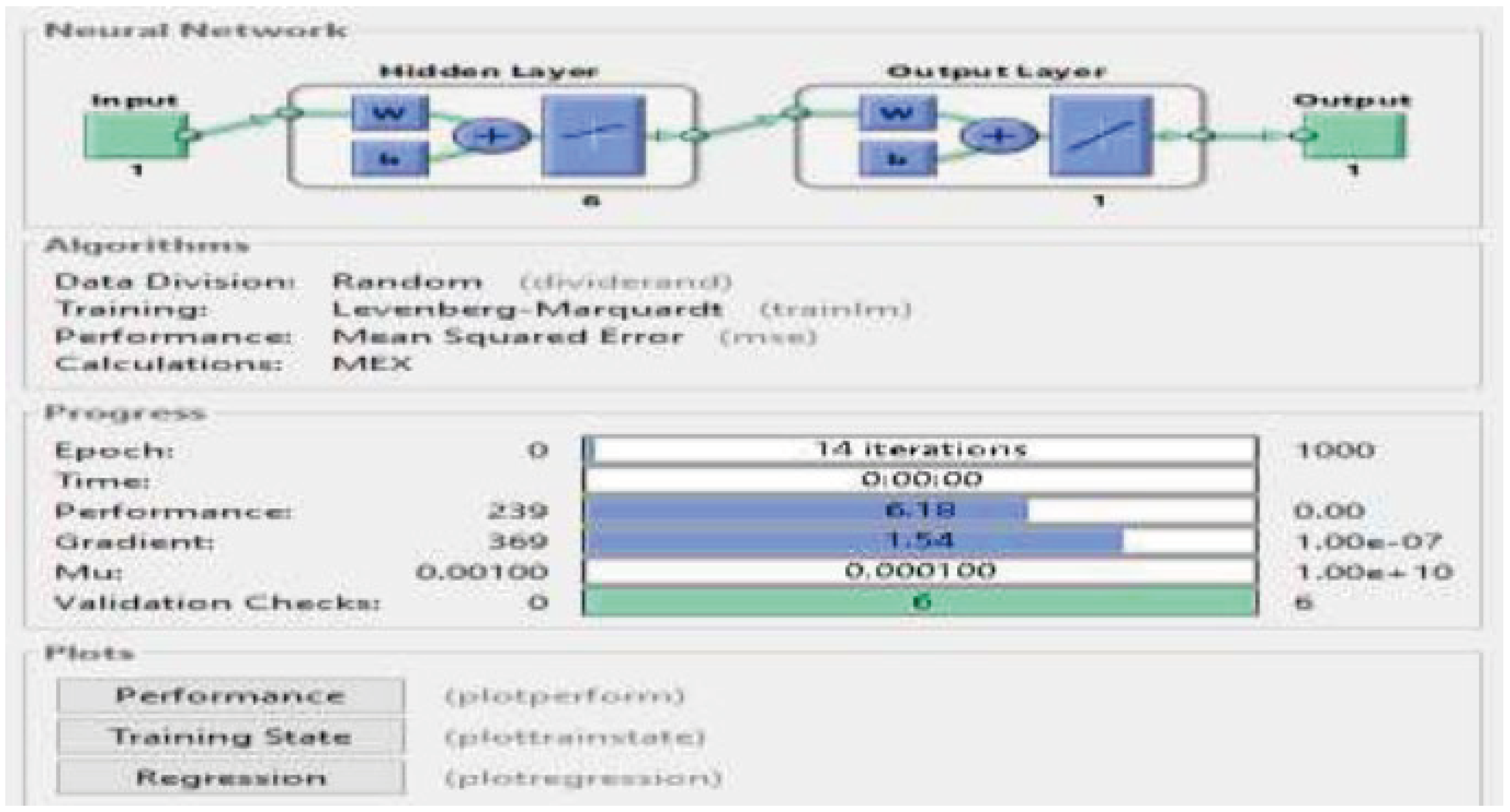
In this paper, the calibration of traffic flow models is investigated for two case studies: Tehran-Karaj Freeway and Tehran-Qom Freeway. Five models are compared, including GreenShields, Greenberg, Pipes, Underwood, and a Multi-Layer Perceptron (MLP) neural network.The methodology involves three main steps. The first step consists of determining the parameters using field data (Dj, Sf). In the second step, the obtained parameters are utilized in the respective models. The third step focuses on evaluating the fit of each model to the dataset by calculating the mean deviation. This involves inserting the data into the model, obtaining the dependent variable, and comparing it with the existing values to calculate error and variance, assessing the accuracy and prediction capability of each model. The MLP model, a fundamental neural network [25] that simulates the transient function of the human brain, is utilized in this study. It is composed of interconnected layers, where input values are multiplied by weights, pass through layers, and generate outputs. The training of the network is conducted using the error propagation method. Figure 1 illustrates the architecture, utilizing the TrainLM training function, a sigmoid function in the first layer, a linear function in the second layer, and Mean Square Error (MSE) for performance evaluation with six hidden neurons. The error propagation algorithm considers the stimulation function as the total weight of inputs related to the neuron. Equation (6) expresses the model, where W represents the weights between the input and next layers. Figure 1 provides an overview of the process, featuring a logistic function (sigmoid) in the first layer and a Purelin function in the second layer.
A j ( x ¯ , w ¯ ) = i = 0 n x i w j i
Each neuron in the first layer multiplies input data (x) by individual weights (W1), capturing feature influence. This sum is then "fired" through an activation function (like sigmoid) to introduce non-linearity and learn complex relationships. The resulting activation becomes the neuron's output. Typically, we split data into 70% for training, 15% for validation, and 15% for testing.
The hidden layer function, represented by the sigmoid function in MATLAB, is expressed in Equation (7). The MATLAB 2016 software is employed for designing and implementing the MLP model, following the same equations for both Tehran-Karaj Freeway and Tehran-Qom Freeway cases.
sigmoid(x) = 1 / (1 + exp(-x)).

3.2. Model Evaluation

MSE is a popular metric for assessing the performance of MLP models [26], especially in regression tasks where continuous values are predicted. It measures the average squared difference between predicted and actual values. MSE connects to the concept of error propagation through the training process. During training, MLPs utilize an algorithm like error propagation to adjust their internal parameters (weights) iteratively. This adjustment aims to minimize the error between predicted and actual values, often calculated using MSE as the loss function (Equation (7)).
M S E ( x ¯ ) = E [ ( x ¯ μ ) 2 ] = ( σ n ) 2 = σ 2 n

3.3. Collection and Analysis

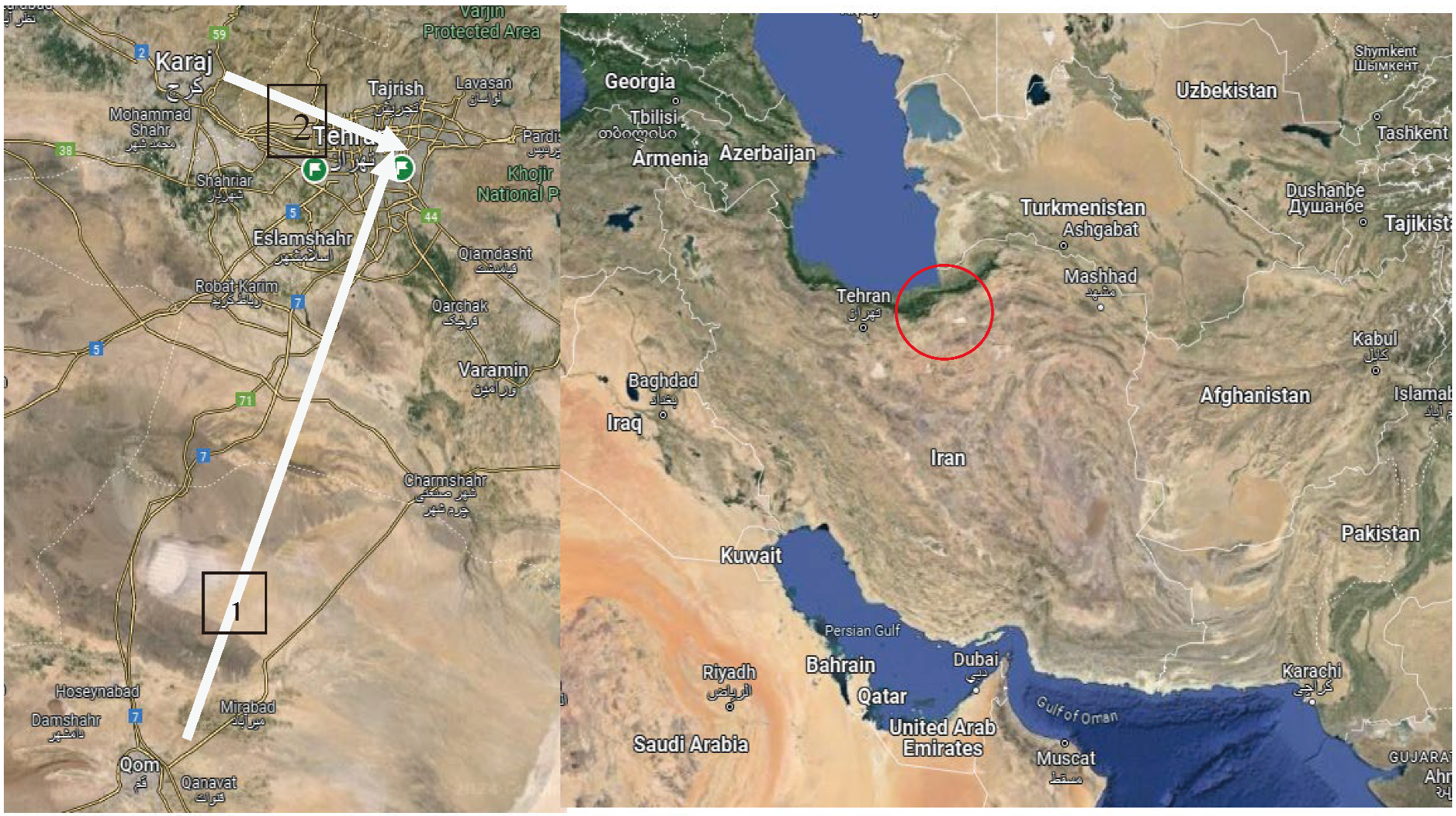
The case study investigates and compares the traffic flow on two major Iranian freeways, namely the Tehran-Karaj Freeway and the Tehran-Qom Freeway. The Tehran-Qom Freeway, spanning 120 kilometers and connecting the two cities, exhibits an average hourly traffic density of 29.01 vehicles/km. In contrast, the Tehran-Karaj Freeway, covering a distance of approximately 30 kilometers between the cities, demonstrates a significantly higher average hourly density of 48.02 vehicles/km. This discrepancy in traffic density highlights the substantial differences in the traffic volumes experienced by the two freeways, with the Tehran-Karaj Freeway notably having a much higher traffic volume than the Tehran-Qom Freeway. Table 1 and Table 2 present samples of data intended for modeling purposes.
The reason for choosing the two freeways of Tehran-Karaj and Tehran-Qom is that the different characteristics are due to the different flow regimes, as will be explained, freeway number 1 has one flow regime and freeway 2 has two flow regimes.
Figure 2. freeway 1 is Tehran-Qom and freeway 2 is Tehran-Karaj.
Preprints 99923 g002

4. Result

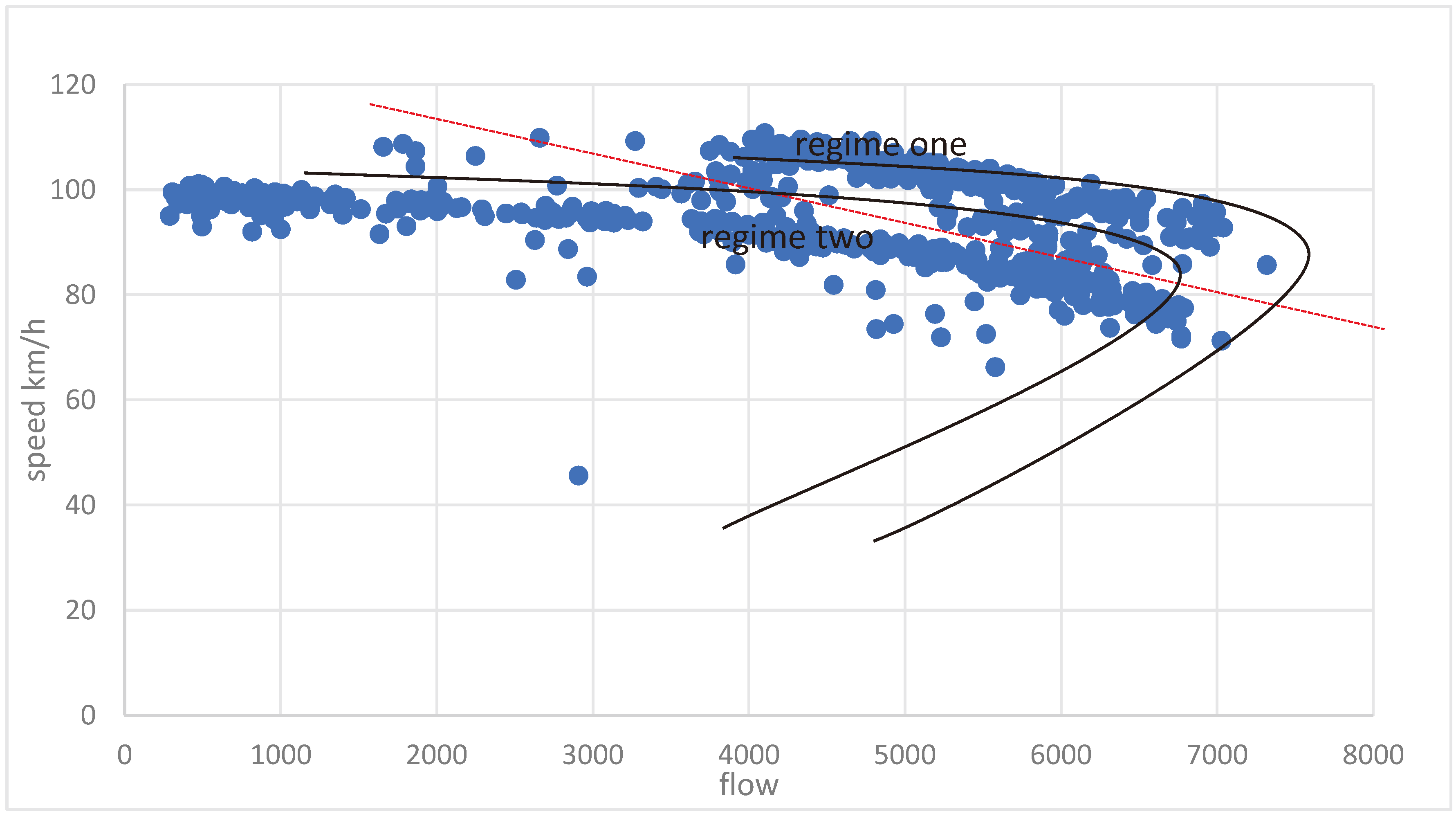
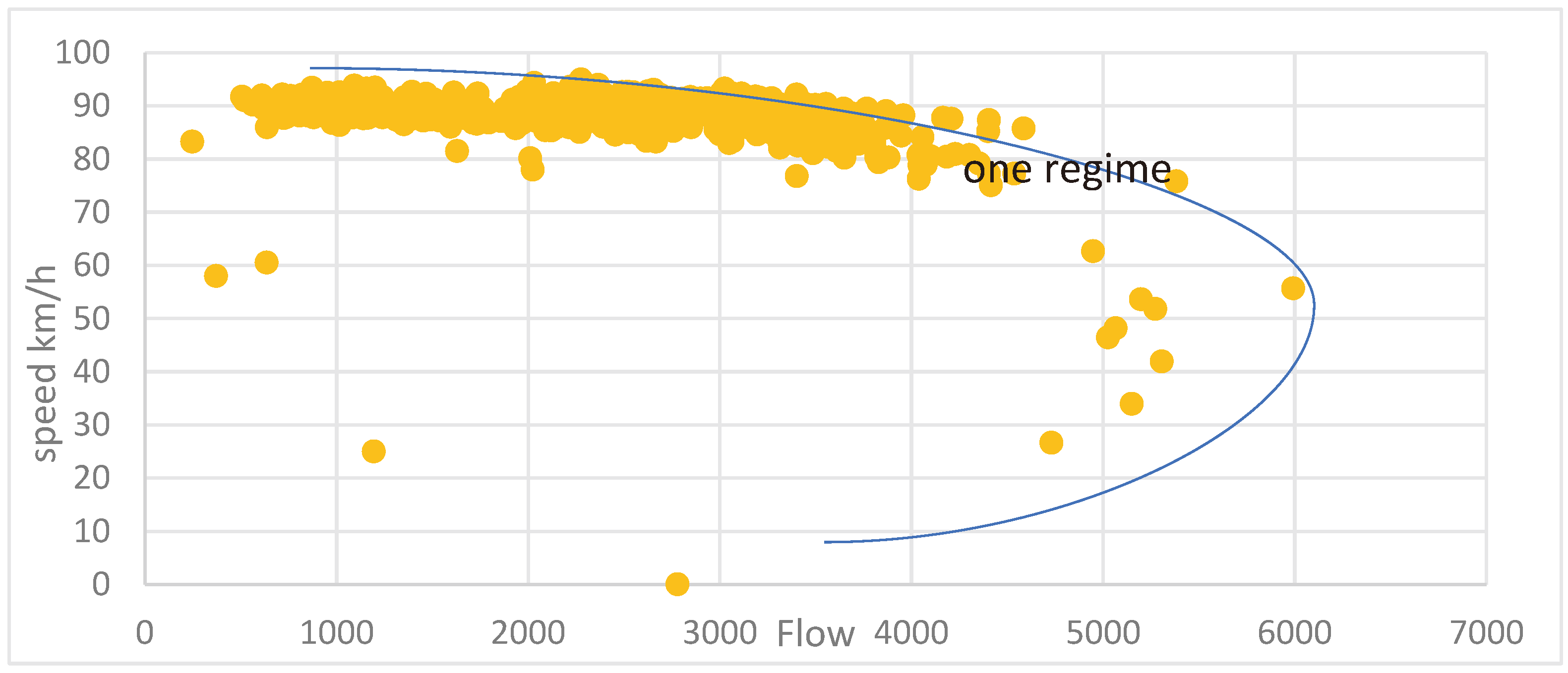
By plotting the flow velocity for both freeways, it becomes evident that one curve adequately represents the flow for freeway one. However, for freeway two, there is a noticeable distinction, with two discernible regimes, aptly named regime one and regime two. It is noteworthy, the second road connecting the two cities, exhibits a high-density flow both during the day and evening.
Figure 3. Flow-speed for Tehran - Qom freeway.
Preprints 99923 g003
The temporal segmentation into two distinct 12-hour periods, from 8 am to 8 pm, introduces a compelling layer to the analysis, revealing the variations in traffic patterns between day and night for both the Tehran-Qom and Tehran-Karaj Freeways. Regime one, associated with daytime flow, and regime two, linked to nighttime flow, showcase distinct characteristics during these timeframes. The red dashed line as a visual demarcation is a valuable addition, effectively partitioning the flow patterns between day and night. This visual cue serves a crucial role in highlighting the precise transition point where the dynamics of traffic flow shift. Its significance lies in providing a clear representation of the temporal distinction between regime one and regime two on the plotted curve for freeway two. By doing so, it enhances the interpretability of the data, enabling readers to discern and analyze the nuanced variations in flow velocity during different periods of the day and night, contributing to a more comprehensive understanding of the freeways' traffic dynamics.
Figure 3. Flow-speed for Tehran - karaj freeway.
Preprints 99923 g003a
The parameters for each model are acquired using the SPSS software. Subsequently, the model is formulated, and standard deviation along with R2 (R-Squared) values are computed and compared.
For the GreenShield Model, the speed is determined for free flow, reaching up to 93.16 km/h, while the traffic jam density (Dj) is established at a maximum of 153.49 pc/km/ln, as indicated in Table 3. By substituting these values into Equation (1), the GreenShield model for the Tehran-Qom freeway is derived, as represented in Equation (8). The ensuing analysis involves the assessment and comparison of standard deviation and R2, providing insights into the model's accuracy and effectiveness in capturing the traffic dynamics of the Tehran-Qom freeway.
S=93(1-D/153)
Continuing the analysis for the Tehran-Karaj highway, Equation (5-2) is obtained, and to streamline the presentation and avoid redundancy, reference is made to the corresponding table (Green Shields Tehran-Karaj).
S=101.8(1-D/234.4)
In the Greenberg's logarithmic model, the necessity for free-flow speed is alleviated, and the crucial parameter becomes the optimal speed denoted c. For the Tehran-Qom freeway, this optimal speed is determined to be 3.9 km per hour. Additionally, the density of traffic jam tends towards infinity. The formulated equation for the Tehran-Qom freeway is presented in Equation (10). Here, S represents the speed, c is the optimal speed parameter, Dj denotes traffic jam density, and D is the traffic density.
S=3.4ln(1+∞/D)
Similarly, for the Tehran-Karaj highway, the optimal speed parameter (c) is found to be 3.4 km per hour, and the traffic jam density tends towards infinity, as indicated in Equation (11).
S=3.4ln(1+∞/D)
Table 4. SPSS software output for the GreenShields model of Tehran -Qom.
Parameter Estimates
Parameter Estimate Std. Error 95% Confidence Interval
Lower Bound Upper Bound
D 35366937919.836 56882385717.037 -76311945740.05 147045821579.72
c 3.945 .287 3.381 4.508
In the Pipes Model, which shares similarities with the GreenShields model, an exploration with different values of the exponent n (specifically n=4,3,2,1) has been conducted. According to the findings presented in Table 5, the best regression line is achieved when n=4, yielding a free-flow speed (Sf) of 89 km/h and a traffic jam density parameter (Kj) of up to 31.6 pc/km/h for the Tehran-Qom Freeway. Substituting these values into the model equation results in Equation (12). For the Tehran-Karaj Freeway, the optimal parameters are Sf =98.5 km/h and K j =43.6 pc/km/ln, as indicated in the same model equation.
S = 89 [1- (D / 31.6) 4]
S = 98.5 [1- (D / 43.6) 4]
In the Underwood's exponential model, two crucial parameters, namely the free-flow speed (Sf) and optimal density (Do), are obtained through the utilization of SPSS software, as detailed in Table 6. It is noted that, to streamline the presentation, the specific table for the Tehran-Karaj Freeway is not reiterated. For the Tehran-Qom Freeway, the free-flow speed is determined to be 87 kilometers per hour, and the optimal density is indicated as infinite, signifying a limitation in this model Similarly, for the Tehran-Karaj Freeway, the parameters are Sf =94.8 km per hour Do =∞.These equations encapsulate the Underwood's exponential model for the Tehran-Qom and Tehran-Karaj freeways, respectively.
S=87.16exp(-d/∞)
S=94.8 exp(-d/∞)
In this model utilizing a multi-layer perceptron (MLP), the Neural Network for both the Tehran-Qom and Tehran-Karaj Freeways is designed with specific characteristics. In Figure 4, the architecture of the network is illustrated, featuring two internal layers. The first layer employs a sigmoid function (logistic function), while the second layer utilizes a linear function. The training process employs the TrainLM training function in MATLAB2016, and the performance evaluation is based on the Mean Square Error (MSE) function
The results of various models are consolidated in Table 7. The findings in this table reveal that the R2 (coefficient of determination) for the neural network model stands out significantly, surpassing the R2 values of other models. This enhanced R2 can be attributed to the low standard deviation of the data for the neural network, indicating the model's robustness and ability to capture the intricate patterns within the freeway's traffic dynamics. The overall analysis suggests that the neural network model outperforms other models, establishing it as the most effective model for both the Tehran-Qom and Tehran-Karaj Freeways.
In Figure 3, it is evident that the traffic flow on the Tehran-Karaj freeway exhibits two distinct regimes. Subsequently, the data was partitioned into two categories, day and night, leading to a reevaluation of the modeling process. Notably, there has been a substantial improvement in the fit of the model. The results (Table 8) specifically pertain to the Tehran-Karaj freeway, indicating that the modeling adjustments based on the day and night categories have contributed significantly to enhancing the accuracy and effectiveness of the traffic flow model for this specific freeway section.
Table 9 provides an overview of the change in R-Square values for different traffic flow models applied to the Tehran-Karaj freeway, considering both one regime and two regimes. This table offers a breakdown of R-Square values for each model, emphasizing distinctions between day and night regimes.

5. Discussions

Single-regime models employ a single mathematical function to depict the relationship between speed, flow, and density across all traffic conditions [9]. In contrast, Multi-regime models utilize distinct functions for different regimes, offering a more accurate portrayal of the intricate relationship within traffic flow characteristics. Identifying these regimes often involves analyzing data based on speed, flow, and density. Methods such as clustering or density-based approaches are commonly employed for regime identification. For instance, a study applied a probabilistic approach with a hidden Markov model to describe similar density characteristics on a freeway [27]. Researchers strategically partitioned traffic flow data into distinct regimes, developing individualized models for each pattern, emphasizing the strategic significance and adaptability of a multi-regime strategy for enhancing forecasting precision [27,28].
The paper highlights a notable shift in R-Square values for various models when transitioning from one regime to two regimes, specifically during day and night periods. The Neural Network Model particularly excels, showcasing substantial improvements in R-Square for both day and night regimes. The distinction between day and night data allows for a nuanced evaluation of each model's performance across different time frames. Models like GreenShields, Greenberg, Pipes, and Underwood exhibit noteworthy enhancements in R-Square values for both day and night, demonstrating their adaptability to diverse traffic patterns. The change in R-Square provides valuable insights into the improved model fit after accounting for distinct regimes. A higher change in R-Square signifies enhanced explanatory power over observed traffic flow data. The consistent high performance of the Neural Network Model underscores its adaptability and proficiency in capturing intricate relationships within traffic dynamics, particularly evident in the two-regime scenario. The study suggests that considering distinct regimes, especially during day and night, significantly enhances modeling accuracy for freeways. These findings have practical implications for traffic management and planning, emphasizing the importance of understanding variations throughout the day for effective decision-making in traffic-related scenarios.
6. Conclusions

In conclusion, the calibration results indicate the challenging nature of consistently fitting empirical data with single-regime models, particularly in varying traffic conditions such as light-traffic/free-flow and congested/jam scenarios. However, this study reveals that the speed-density relationship can be effectively represented by single-regime models when utilizing distinct data for day and night conditions. With properly developed functional forms and calibration approaches, single-regime models exhibit surprising efficacy. Moreover, the observed dispersion can be meaningfully categorized into two distinct groups: day and night. By analyzing freeway data separately for day and night, a notable reduction in errors across all models, particularly in the Tehran-Qom freeway models, is achieved. This reduction in errors is attributed to the lower dispersion of the traffic rate parameter between day and night. Implementing this parameter across all models could significantly enhance overall accuracy. Notably, the neural network model outperforms other models, emphasizing the superiority of dynamic models over static ones. The application of the day and night parameter to the neural network model is suggested to further increase accuracy, aligning it with the performance of other models. In summary, the change in R-Square values and the model-specific performance under different regimes offer crucial insights into the adaptability and effectiveness of traffic flow models for the Tehran-Karaj freeway. The findings underscore the importance of considering distinct regimes to improve the models' representation of the intricacies within traffic dynamics in this specific context.

Author Contributions

Parisa Raufi - Writing, Review, data curation and Editing; Mohammad Maniat - Methodology, Conceptualization. All authors have read and agreed to the published version of the manuscript.

Data Availability Statement

The data presented in this study are available on reasonable request from the corresponding author.

Conflicts of Interest

The authors declare that there is no conflict of interest.

References

  1. MrcrlAloPoulos, P.G. Analysis of traffic flow at complex congested arterials. Trffic Flow Theory ønd 1988, 1, 77. [Google Scholar]
  2. Zeb, A.; et al. HetroTraffSim: A Macroscopic Heterogeneous Traffic Flow Simulator for Road Bottlenecks. Future Transportation 2023, 3, 368–383. [Google Scholar] [CrossRef]
  3. Khan; Z. H.; Gulliver, T.A. A macroscopic traffic model for traffic flow harmonization. European Transport Research Review 2018, 10, 1–12. [Google Scholar]
  4. Mahapatra, G.; Maurya, A.K.; Chakroborty, P. Parametric study of microscopic two-dimensional traffic flow models: A literature review. Canadian Journal of Civil Engineering 2018, 45, 909–921. [Google Scholar] [CrossRef]
  5. van Wageningen-Kessels, F.; et al. Genealogy of traffic flow models. EURO Journal on Transportation and Logistics 2015, 4, 445–473. [Google Scholar] [CrossRef]
  6. Elefteriadou, L. An introduction to traffic flow theory. 2014: Springer.
  7. Kerner, B.S. Understanding Real Traffic. 2021: Springer.
  8. Reilly, W. Highway capacity manual 2000. Tr News, 1997(193).
  9. Qu, X.; Wang, S.; Zhang, J. On the fundamental diagram for freeway traffic: A novel calibration approach for single-regime models. Transportation Research Part B: Methodological 2015, 73, 91–102. [Google Scholar] [CrossRef]
  10. Yugendar, P.; Ravishankar, K.V.R. Multi-regime modelling of large congregations. in Proceedings of the Institution of Civil Engineers-Transport. 2021. Thomas Telford Ltd.
  11. Sun, L.; Zhou, J. Development of multiregime speed–density relationships by cluster analysis. Transportation Research Record 2005, 1934, 64–71. [Google Scholar] [CrossRef]
  12. Kidando, E.; et al. Novel approach for calibrating freeway highway multi-regimes fundamental diagram. Transportation Research Record 2020, 2674, 561–574. [Google Scholar] [CrossRef]
  13. Maniat, M.; Eebrahimzadeh, A. Enhancing Traffic Prediction Accuracy: A Comparative Analysis of Data Quality and Model Evaluation Using Artificial Intelligence. 2024.
  14. Greenshields, B.D.; et al. A study of traffic capacity. in Highway research board proceedings. 1935. Washington, DC.
  15. Lighthill, M.J.; Whitham, G.B. On kinematic waves II. A theory of traffic flow on long crowded roads. Proceedings of the Royal Society of London. Series A. Mathematical and Physical Sciences 1955, 229, 317–345. [Google Scholar]
  16. Phillips, W.F. A kinetic model for traffic flow with continuum implications. Transportation Planning and Technology 1979, 5, 131–138. [Google Scholar] [CrossRef]
  17. Pipes, L.A. An operational analysis of traffic dynamics. Journal of applied physics 1953, 24, 274–281. [Google Scholar] [CrossRef]
  18. Ali, F.; et al. A Microscopic Traffic Model Considering Time Headway and Distance Headway. Applied Sciences 2023, 13, 7234. [Google Scholar] [CrossRef]
  19. Salter, R.; Salter, R. The relationship between speed, flow and density of a highway traffic stream. Highway Traffic Analysis and Design 1976, 125–134. [Google Scholar]
  20. Underwood, R.T. Speed, volume and density relationships, in quality and theory of traffic flow. Bur. Highway Traffic, Yale Univ. 1961, 141-188.
  21. Greenberg, H. An analysis of traffic flow. Operations research 1959, 7, 79–85. [Google Scholar] [CrossRef]
  22. Zhang, J. Probabilistic modelling for flow density relationship. 2018.
  23. Bramich, D.M.; Menéndez, M.; Ambühl, L. Fitting empirical fundamental diagrams of road traffic: A comprehensive review and comparison of models using an extensive data set. IEEE Transactions on Intelligent Transportation Systems 2022, 23, 14104–14127. [Google Scholar] [CrossRef]
  24. Wang, J.; Boukerche, A. Non-parametric models with optimized training strategy for vehicles traffic flow prediction. Computer Networks 2021, 187, 107791. [Google Scholar] [CrossRef]
  25. Oliveira, D.D.; et al. Forecasting vehicular traffic flow using MLP and LSTM. Neural Computing and applications 2021, 33, 17245–17256. [Google Scholar] [CrossRef]
  26. Dessain, J. Machine learning models predicting returns: Why most popular performance metrics are misleading and proposal for an efficient metric. Expert Systems with Applications 2022, 199, 116970. [Google Scholar] [CrossRef]
  27. Lu, Z.; et al. Short-term traffic flow forecasting via multi-regime modeling and ensemble learning. Applied Sciences 2020, 10, 356. [Google Scholar] [CrossRef]
  28. Li, Z.; Li, Y.; Li, L. A comparison of detrending models and multi-regime models for traffic flow prediction. IEEE Intelligent Transportation Systems Magazine 2014, 6, 34–44. [Google Scholar]
Figure 1. The designed neural network model and its functions.
Preprints 99923 g001
Figure 4. Neural Network Model in MATLAB Software for Tehran-Qom Freeway.
Preprints 99923 g004
Table 1. Sample of Traffic Data for Tehran-Qom Roads, Source: National Road Organization Iran.
Free Way Name Time Number of Vehicles (Hourly) Average Speed (Hourly) Density
Tehran-Qom 2020/06/01 00:00:00 1632 86.43 18.88
Tehran-Qom 2020/06/01 01:00:00 1226 86.59 14.16
Tehran-Qom 2020/06/01 02:00:00 816 88.99 9.17
Tehran-Qom 2020/06/01 03:00:00 708 89.92 7.87
Tehran-Qom 2020/06/01 04:00:00 694 93.71 7.41
Tehran-Qom 2020/06/01 05:00:00 998 91.52 10.9
Tehran-Qom 2020/06/01 06:00:00 2156 91.21 23.64
Tehran-Qom 2020/06/01 07:00:00 3336 91.06 36.64
Tehran-Qom 2020/06/01 08:00:00 3084 92.04 33.51
Tehran-Qom 2020/06/01 09:00:00 2518 92.17 27.32
Tehran-Qom 2020/06/01 10:00:00 2615 91.22 28.67
Tehran-Qom 2020/06/01 11:00:00 2355 91.63 25.7
Tehran-Qom 2020/06/01 12:00:00 2415 90.25 26.76
Continue until the end of the table for 31 days . . . .
days, including 744 row . . . .
Average 2527.26 87.13 29.01
Table 2. Sample of Traffic Data for Tehran-Karaj Roads, Source: National Road Organization Iran.
Free Way Name Time Number of Vehicles Average Speed Density
Tehran -Karaj 2020/06/01 00:00:00 2906 95.6 30.4
Tehran -Karaj 2020/06/01 01:00:00 1759 97.05 18.12
Tehran -Karaj 2020/06/01 02:00:00 904 97.15 9.31
Tehran -Karaj 2020/06/01 03:00:00 542 98.79 5.49
Tehran -Karaj 2020/06/01 04:00:00 707 98.51 7.18
Tehran -Karaj 2020/06/01 05:00:00 1175 99.59 11.8
Tehran -Karaj 2020/06/01 06:00:00 3851 100.27 38.41
Tehran -Karaj 2020/06/01 07:00:00 5545 94.37 58.76
Tehran -Karaj 2020/06/01 08:00:00 5122 94.98 53.93
Tehran -Karaj 2020/06/01 09:00:00 5082 97.76 51.98
Tehran -Karaj 2020/06/01 10:00:00 5212 97.92 53.23
Tehran -Karaj 2020/06/01 11:00:00 4960 104.53 47.45
Tehran -Karaj 2020/06/01 12:00:00 5094 105.05 48.49
Continue until the end of the table for 31 days . . . .
days, including 744 row . . . .
Average 4493.96 94.82 48.02
Table 3. SPSS software output for the Tehran -Qom GreenShields Model.
Parameter Estimate Std.Error 95%Confidence Interval
Lower Bound Upper Bound
S 93.16 0.32 92.51 93.8
D 153.49 7.29 139.18 167.81
Table 5. SPSS software output for the Pipes Model of Tehran -Qom.
Parameter Estimate Std. Error 95%Confidence Interval
Lower Bound Upper Bound
S 88.97 0.122 88.73 89.21
D 31.61 0.269 31.08 32.14
Table 6. SPSS software output for the Underwood Model Tehran -Qom.
Parameter Estimate Std. Error 95%Confidence Interval
Lower Bound Upper Bound
S 87.16 0.162 86.88 87.48
Do 9858665281 2.46E+15 -4.83E+15 4.83E+15
Table 7. Comparison of Model Performance for Tehran-Karaj and Tehran-Qom Freeways.
Tehran-Karaj Tehran-Qom
Model R-Squre Standard Deviation R-Squre Standard Deviation
GreenShields 0.194 6.01 0.35 3.3
Greenberg 0.11 6.4 0.21 3.6
Pipes 0.33 6.8 0.8 12
Underwood 0.194 6.8 0.19 6.8
neural network 0.76 5.1 0.82 2.5
Table 8. Model Performance for Tehran-Karaj freeway after distinct regimes.
Tehran-Karaj Day Tehran-Karaj Night
Model R-Squre Standard Deviation R-Squre Standard Deviation
GreenShields 0.78 3.2 0.79 3.2
Greenberg 0.64 3.4 0.65 3.3
Pipes 0.85 2.5 0.84 2.4
Underwood 0.71 3.5 0.72 2.9
neural network 0.95 1.6 0.96 1.6
Table 9. Change in R-Squre for Tehran-Karaj freeway after distinct regimes.
Tehran-Karaj
Type One Regime Two Regime
Model R-Squre R-Squre Day R-Squre Night Change R-Squre
GreenShields 0.194 0.78 0.79 0.60
Greenberg 0.11 0.64 0.65 0.54
Pipes 0.33 0.85 0.84 0.51
Underwood 0.194 0.71 0.72 0.53
neural network 0.76 0.95 0.96 0.20
Disclaimer/Publisher’s Note: The statements, opinions and data contained in all publications are solely those of the individual author(s) and contributor(s) and not of MDPI and/or the editor(s). MDPI and/or the editor(s) disclaim responsibility for any injury to people or property resulting from any ideas, methods, instructions or products referred to in the content.
Copyright: This open access article is published under a Creative Commons CC BY 4.0 license, which permit the free download, distribution, and reuse, provided that the author and preprint are cited in any reuse.
Prerpints.org logo

Preprints.org is a free preprint server supported by MDPI in Basel, Switzerland.

Subscribe

© 2024 MDPI (Basel, Switzerland) unless otherwise stated