Time Series Forecasting with Missing Values Using Multiple Models: An Application to Wind Energy Systems

Preprint

Article

Time Series Forecasting with Missing Values Using Multiple Models: An Application to Wind Energy Systems

Altmetrics

Downloads

Views

Comments

Xiaoou Li^*

This version is not peer-reviewed

Submitted:

27 February 2024

Posted:

28 February 2024

You are already at the latest version

Alerts

Abstract

When dealing with limited sample sizes or missing values in time series data, achieving high accuracy in forecasting becomes challenging. This challenge is particularly common in wind energy forecasting, where many wind farms lack complete data. In this paper, we employ the widely-used ARIMA (Autoregressive Integrated Moving Average) model for time series forecasting. To address the difficulties posed by limited sample sizes and missing values, we adopt a unique approach by utilizing multiple ARIMA models for different datasets. A key distinction from other multiple models methods for time series forecasting lies in each model within our approach using its own dataset, making the fusion process more intricate. To overcome this, we incorporate neural networks and two techniques for model fusion: direct fusion with a learning mechanism and compensation for missing data through training. For each ARIMA model, we introduce a noise estimation method to circumvent the white noise assumptions inherent in ARIMA models. Finally, we apply these methods to wind energy prediction, and our experimental results showcase a significant enhancement in forecasting accuracy.

Keywords:

Subject: Computer Science and Mathematics - Artificial Intelligence and Machine Learning

1. Introduction

The ARIMA (Autoregressive Integrated Moving Average) model is widely employed for time series forecasting, particularly in the context of non-stationary time series like wind energy. Utilizing ARIMA for wind energy prediction can enhance the reliability and quality of wind power generation [1]. This model captures the temporal correlation and probability distribution of time series by separating high and low frequencies [2]. In [3], the autocorrelation function is employed to determine the structure of the ARIMA model, while [4] improves ARIMA prediction accuracy by integrating aerodynamic atmospheric models. Yumeng’s analysis in [5] applies the ARIMA model to multivariate time series but falls short in achieving satisfactory accuracy for long-term predictions.

The presence of missing values in time series data significantly impacts prediction accuracy. Effectively handling these issues is crucial for reliable results [6]. Various methods have been developed to address missing values, categorized into two groups: physical and statistical approaches [7]. These methods can be applied across different time scales for wind energy forecasting, with statistical methods primarily used for complete datasets and physical methods for those with missing values [8]. To address the challenges of gas recognition in E-nose systems with limited labeled data, a Domain Adaptation Neural Network is proposed, emphasizing robust classification while maintaining efficiency and learning ability [9]. Ye et al. tackle wide variability between old and new data in time series prediction by combining transfer learning and ensemble learning, effectively leveraging historical data and latent knowledge for current predictions [10]. In recent years, Long Short-Term Memory (LSTM) neural networks have gained popularity as an alternative to traditional models due to their capacity to handle missing data in time series and their nonlinear predictive capabilities [11].

Another contributing factor to the low accuracy with missing values lies in the linearity of the ARIMA model. However, the nonlinear models, such as Neural Networks (NN), have gained popularity and demonstrated success in wind energy forecasting applications [12]. These models incorporate long-term memory activation functions and utilize optimization algorithms. Additionally, Multilayer Perceptrons and Radial Basis Function Neural Networks have been effectively applied for wind speed prediction [13]. Bayesian regularization, Levenberg Marquardt, and Recursive Neural Networks have found application in other studies [14,15]. Various other nonlinear models have been explored for prediction with missing data, including Reinforcement Learning [16], Fuzzy Logic [17], and Support Vector Machines [18]. In [19], the combination of Empirical Mode Decomposition and Local Mean Decomposition complements each other, reducing errors in decomposition and enhancing the efficiency of Support Vector Machines, along with improving the accuracy of Stochastic Configuration Networks for large datasets. Furthermore, [20] proposes four hybrid methods for multi-step wind speed predictions, leveraging Adaboost and MLP Neural Networks. Due to the intricate nature of neural networks, interpreting them can be challenging. As indicated by the findings presented in [21], none of the nonlinear models have exhibited a significant improvement over linear models for time series forcasting.

Another approach to enhance forecasting accuracy in time series prediction involves utilizing multiple models. In [22], a multiple models method was introduced to enhance accuracy, particularly for very short-term wind speed forecasting. Gupta [23] combined deep wavelet decomposition with a feedback instrument, while others combined ARIMA with artificial neural networks. For instance, the ARIMA model is integrated to define the NN model in [24]. Soham [25] proposed a hybrid model, combining ARIMA with a dynamically evolving fuzzy neural inference system. Hybrid neural networks proposed by Mehdi [26] and Aly [27] incorporated the clonal selection algorithm, particle swarm optimization, and extreme learning machine

However, all of these multiple ARIMA models can only utilize a single dataset. When this dataset contains missing values, they are rendered ineffective, as noted by [28]. To address the issue of missing values, transfer learning and ensemble learning have proven effective, as suggested by [6]. Additionally, [9] proposes domain adaptation using limited labeled data. In [10], the problem of wide variability between old and new data in time series prediction was resolved using ensemble learning. However, for common problems in time series forecasting, such as missing values, conclusive results are still lacking.

To enhance the accuracy with missing values, we employ a multiple-model technique and neural networks in conjunction with the ARIMA model. We augment the training data using datasets from other wind farms. By fusing models from several wind farms with neural networks, we integrate knowledge from different monitoring locations to address the training problem arising from missing data. This paper makes the following contributions:

We propose an effective training method for a single ARIMA model. We use the noise estimation method, popular in adaptive control, to estimate the coefficients of the ARIMA model. One significant advantage over other ARIMA training methods is that we no longer assume the noise to be weak white noise.
We address the problem of low forecasting accuracy with missing data. By using multiple models and neural networks, we propose a novel multiple ARIMA that significantly improves the prediction accuracy of time series forecasting. To the best of our knowledge, this is the first time that multiple ARIMAs have been trained on different datasets.
The proposed multiple ARIMA models are successfully applied to wind energy prediction

2. Single Linear Model for Time Series Forecasting Using Noise Estimation

2.1. ARIMA Linear Model

The ARIMA model is an extended version of the ARMA (AutoRegressive Moving Average) model that incorporates an integration component. This model consists of three stages [2]:

(1) AutoRegressive (AR). It expresses the past values of time series

\{y_{t}\}

y_{t} = a_{0} + a_{1} y_{t - 1} + . . . + a_{p} y_{t - p} + ϵ_{t}

(1)

where

a_{i}

are the coefficients of the linear AR model,

ϵ_{t}

is white noise. It has zero mean and independent and identically distributed (i.i.d.)

(2) Moving Average (MA). It expresses the past values of noise

ϵ_{t}

y_{t} = ϵ_{t} + b_{1} ϵ_{t - 1} + . . . + b_{q} ϵ_{t - q}

(2)

(3) Integration (I). Stationarity is a critical factor in time series forecasting and a key parameter for designing the ARIMA model. We calculate the difference as

Δ y_{t} = y_{t} - y_{t - 1}

(3)

It introduces differentiation to smoothen the time series and make it closer to being stationary.

The zero mean

(p, q)

-order ARMA model is

(1 - a_{0}) y_{t} = a_{1} y_{t - 1} + . . . + a_{p} y_{t - p} + ϵ_{t} + b_{1} ϵ_{t - 1} + . . . + b_{q} ϵ_{t - q}

(4)

Let z be the lag operator

z^{- 1} y_{t} = y_{t - 1}, z^{- 2} y_{t} = y_{t - 2}

d-order integration can be defined as

y_{t} = ▽^{d} x_{t} = {(1 - z^{- 1})}^{d} x_{t}

(p, q, d)

-order ARIMA model is

(1 - \sum_{k = 1}^{p} a_{i} z^{- k}) {(1 - z^{- 1})}^{d} y_{t} = (1 + \sum_{k = 1}^{q} b_{j} z^{- k}) ϵ_{t}

(5)

The parameters of the

(p, q, d)

-order ARIMA model are

θ = [a_{1} \dots a_{p}, b_{1} \dots b_{q}]

(6)

2.2. Structure of the Linear Model

Time series forecasting entails predicting future values based on past values of a time series with a certain degree of precision. It involves a process of time series modeling, where the objective of utilizing ARIMA models is to identify a suitable ARIMA model (5), such that the prediction error, defined as:

e_{t} = y_{t} - y_{t}^{*}

is minimized. Here,

y_{t} = A R I M A_{θ} (p, q, d)

represents the output of the ARIMA model,

y_{t}^{*}

is the real vaule.

Time series modeling comprises two main components:

Structure determination: This involves finding optimal model orders $p,$ q and d, such that $(p, q, d)$ -ARIMA model exhibits the best forecasting accuracy with fixed parameters $θ$ ,

$(p, q, d) = min_{p, q, d} \{{[A R I M A_{θ} (p, q, d) - y_{t}]}^{2}\}$

(7)
Parameter estimation: This step entails estimating the model parameters $θ$ , so that the ARIMA model achieves the best forecasting accuracy with a fixed structure $(p, q, d)$

$θ = min_{θ} \{{[A R I M A_{θ} (p, q, d) - y_{t}]}^{2}\}$

(8)

It is impractical to obtain the optimal

A R I M A_{θ^{*}} (p^{*}, q^{*}, d^{*})

model since structure determination as in (7) requires the optimal parameter

θ^{*},

while the parameter estimation (8) requires the optimal structure

(p^{*}, q^{*}, d^{*})

Traditionally, the random walk method is employed to determine the ARIMA structure

(p, q, d),

after which the obtained structure is used to estimate the parameters

θ

using the training data. If the forecasting accuracy proves unsatisfactory, the random walk method is applied iteratively to find alternative

(p, q, d)

combination. This iterative process continues until the forecasting error is sufficiently minimized, although it can be time-consuming and inefficient.

Generally, finding the optimal ARIMA structure is not feasible. Hence, the Akaike Information Criterion (AIC) and Bayesian Information Criterion (BIC) are used as criteria for determining

(p, q, d)

. Both criteria aim to evaluate the trade-off between training error and model complexity, seeking a model that is simple yet accurately fits the training data.

Assuming the data set D consists of N data

y_{1}, \dots, y_{N}

, the AIC and BIC are calculated as follows:

AIC : 2 (p + q + 1) - 2 L, BIC : ln (N) (p + q + 1) - 2 L

(9)

Here,

(p + q + 1)

is the number of the structure parameters of

A R I M A (p, q, d)

L

represents the maximum likelihood value for the ARIMA model, estimated by:

L = N ln (\frac{1}{N} \sum_{t = 1}^{N} e_{t}^{2})

where

e_{t} = y_{t} - y_{t}^{*},

{\hat{y}}_{t}

is the output of the ARIMA model.

In the context of AIC (9), models with lower AIC scores are preferred as AIC penalizes models with more structural parameters. Therefore, if two models are compared on the same time series, the one with a lower

p + q

value will be favored due to its lower AIC score.

2.3. Time Series Forecasting Using Noise Estimation

If the noise

ϵ_{t}

is assumed to be white noise, there is no need for estimation. However, in most time series, it is not reasonable to assume it follows a Gaussian distribution. In this paper, we employ a separate regression method to estimate the noise and simultaneously estimate the parameter

θ .

Once

(p, q, d)

are determined, we can use least square method to estimate the parameter

θ .

For the i-th data

θ (i) = [a_{1} (i) \dots a_{p} (i), b_{1} (i) \dots b_{q} (i)], i = 1 \dots N

(10)

where n is the data size, the ARIMA model (5) in vector form is

y_{t} = [\begin{matrix} a_{1} & \dots & a_{p} & b_{1} & \dots & b_{q} \end{matrix}] [\begin{matrix} x_{t - 1} \\ ⋮ \\ x_{t - p} \\ ϵ_{t} \\ ⋮ \\ ϵ_{t - q} \end{matrix}]

(11)

The noises

ϵ_{t - k},

k = 0 \dots q,

are not available, but we can estimate them using their prior values as

{\hat{ϵ}}_{t} = y_{t} - (\sum_{k = 1}^{p} a_{k} z^{- k}) y_{t}^{*} - (\sum_{k = 1}^{q} b_{k} z^{- k}) {\hat{ϵ}}_{t}

(12)

Then ARMA model (11) becomes

Y = θ \bar{Y} + E

(13)

where

Y = {[y_{t - 1}^{*} \dots y_{t - p}^{*}, {\hat{ϵ}}_{t} \dots {\hat{ϵ}}_{t - q}]}^{T}, \bar{Y} = [\begin{matrix} y_{1, 1} & \dots & y_{1, N} \\ ⋮ & ⋮ \\ y_{p, 1} & y_{p, N} \\ {\hat{ϵ}}_{1, 1} & {\hat{ϵ}}_{1, N} \\ ⋮ \\ {\hat{ϵ}}_{q, 1} & \dots & {\hat{ϵ}}_{q, N} \end{matrix}]

E = [\begin{matrix} e_{1} & \dots & e_{p + q} \end{matrix}]

is the residual error vector. The objective of the parameter identification is

min_{θ} {∥ Y_{t} - θ \bar{Y} ∥}^{2}

(14)

Because (13) is a linear-in-parameter process, the optimal solution of

θ

θ = {[\bar{Y} {\bar{Y}}^{T}]}^{- 1} {\bar{Y}}^{T} Y

(15)

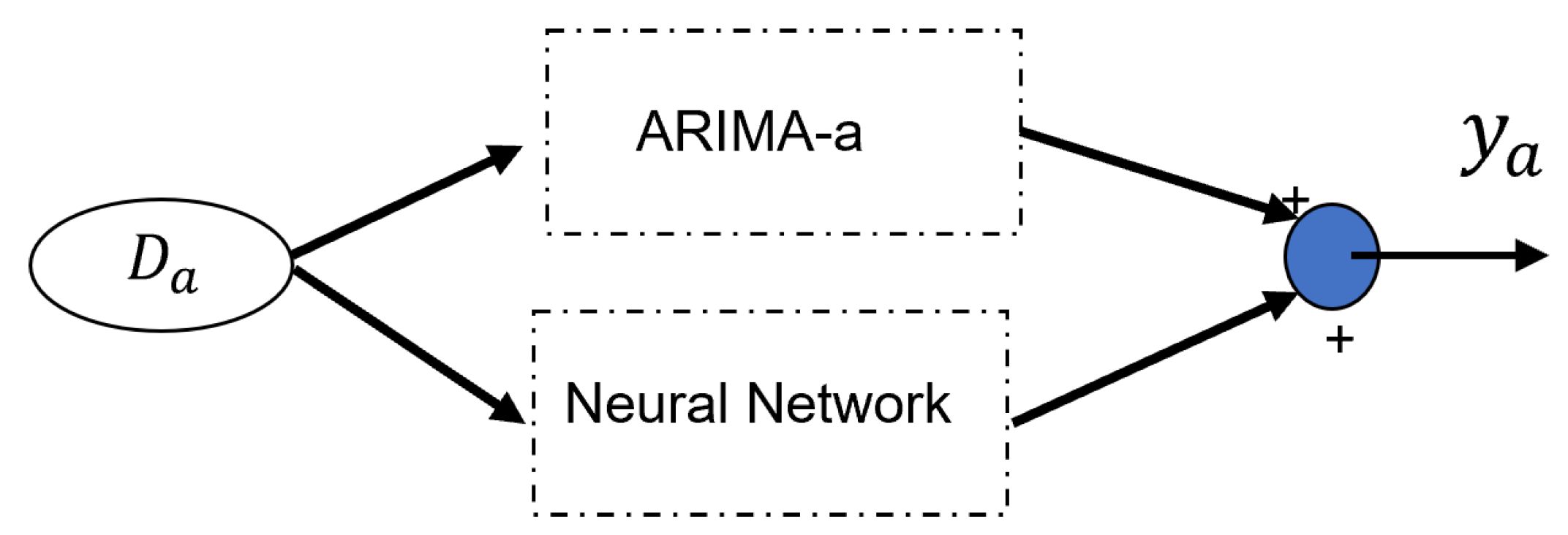
Finally, we obtain a single ARIMA model along with its historical data. The ARIMA model process for time series forecasting is illustrated in Figure 1 and Algorithm 1.

Algorithm 1 Single ARIMA model training

1:: Perform data pre-processing.
2:: Use the Dickey-Fuller method (ADF) to obtain stationary data.
3:: Use the Akaike Information Criterion (AIC) and the Bayesian Information Criterion (BIC) to determine the structure parameter.
4:: Use the least squares method to identify the coefficients (15).
5:: Return the single ARIMA model.

3. Multiple ARIMA Models with Neural Networks

3.1. Limitations of ARIMA and the Other Approaches

The ARIMA model excels in forecasting non-stationary time series, but its performance can suffer when dealing with missing data, high noise levels, or limited samples. This paper proposes utilizing multiple ARIMA models trained on different data sets to enhance forecasting accuracy.The ARIMA model is effective for non-stationary time series forecasting, but it may not work well when the training data sets have missing data, high noise, or small sample sizes. In this paper, we propose using multiple ARIMA models with different data sets to improve the accuracy of forecasting.

3.2. Multiple ARIMA Models

Given l distinct data sets, denoted as:

\{y_{t}^{σ}\}, σ = {1, 2, . . ., l}

we can train l ARIMA models (

M_{1} \dots M_{l}

) using the single ARIMA modeling approach outlined earlier. For each data set

σ

, the optimal

(p, q, d)

parameters are determined using AIC and BIC, followed by parameter estimation for each

(p, q, d)

-order ARIMA model via the least squares method (15).

Each ARIMA model is associated with a parameter vector

θ^{i}

. These multiple ARIMAs are represented as:

A R I M A_{θ^{i}} (p^{i}, q^{i}, d^{i}), i \in σ

(16)

where

θ^{i}

represents the estimated parameters for the i-th ARIMA model. Each ARIMA model,

A R I M A_{θ^{i}} (p^{i}, q^{i}, d^{i})

, is capable of predicting its corresponding data set

\{y_{t}^{i}\} .

3.2.1. Transfer Learning for Robust ARIMA Models

Traditional ARIMA models struggle with uncertainties like missing data, hindering their forecasting accuracy. To overcome this, we propose a novel approach leveraging transfer learning and multiple models.

Transfer learning capitalizes on pre-trained models to accelerate learning when data is limited. In this context, we utilize data from similar but complete domains (denoted as

Λ_{a}

and

Λ_{b}

) to compensate for missing information in the target domain (

Λ_{a}

Formally,

Λ_{a}

and

Λ_{b}

represent matrices of past observations (e.g.,

y_{a} (t - 1), y_{a} (t - 2), . . .,

)

\begin{matrix} Λ_{a} = Y_{a} (t) = [y_{a} (t - 1), y_{a} (t - 2), . . ., y_{a} (t - n)] \\ Λ_{b} = Y_{b} (t) = [y_{b} (t - 1), y_{b} (t - 2), . . ., y_{b} (t - n)] \end{matrix}

(17)

capturing the temporal dynamics of each domain. We exploit the inherent relationship between these domains to extract knowledge from

Λ_{b}

and fill the gaps in

Λ_{a}

Two strategies can be employed:

Joint Training: Train model $M_{a}$ directly using both datasets { $Λ_{a}$ , $Λ_{b}$ }.
Pre-training and Fine-tuning: Pre-train $M_{a}$ with the complete data $Λ_{b}$ , then fine-tune it with the target data $Λ_{a}$ .

Crucially, successful learning hinges on transferring features from the information-rich domain to the data-scarce one.

3.2.2. Generalizing to Multiple Models

This approach extends to l prediction models and their corresponding datasets {

Λ_{i}, \dots Λ_{l}

}. Each prediction task is modeled by an ARIMA equation utilizing past observations:

{\hat{y}}_{i} (t) = A R I M A_{i} [({\hat{y}}_{i} (t - 1), {\hat{y}}_{i} (t - 2), . . ., {\hat{y}}_{i} (t - n)]

(18)

where

σ

represents the domain index.

We define S as a bounded parameter space for each

A R I M A_{i} (D_{i})

model (where

D_{i}

is the i-th dataset). Each model has a parameter vector

θ^{i} \in S

, and we identify

θ^{i *}

as a sub-optimal parameter set within a closed region

Ω \in S

This framework allows us to combine and leverage multiple ARIMA models (

M_{i}

) across different domains, even with varying levels of data availability.

3.3. Combining ARIMA and Neural Networks for Enhanced Forecasting

While ARIMA models excel in time series analysis, their flexibility can be limited, especially with missing data or noisy environments. This paper proposes two novel integration methods combining ARIMA with neural networks to improve forecasting accuracy.

Limitations of Single ARIMA Models:

While ARIMA models excel in capturing temporal patterns in data, they can struggle with limitations like: 1) Limited flexibility: They may not be able to adapt to highly non-linear relationships or complex dynamics. 2) Missing data: Incomplete datasets can significantly impact their accuracy.

Combining ARIMA and Neural Networks:

Our approach addresses these limitations by combining the strengths of both models: (1) ARIMA’s strong performance on time series analysis. (2) Neural networks’ ability to learn complex non-linear relationships.

We propose two novel methods for combining ARIMA and neural networks:

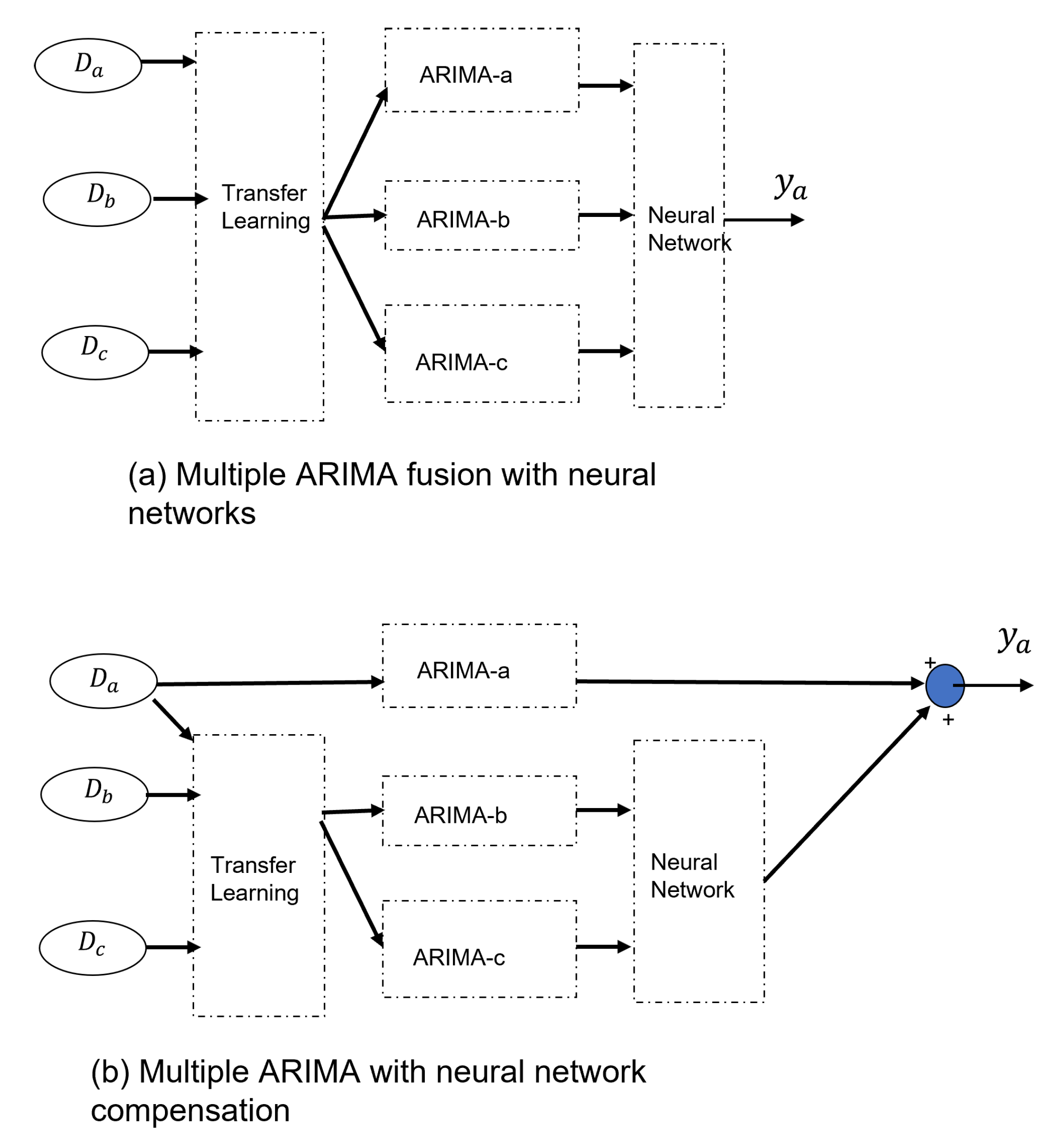
Multiple ARIMA Fusion with Neural Network

This method utilizes multiple ARIMA models trained on different datasets.
The outputs of these models are combined as input to a neural network.
The neural network extracts valuable features and patterns from each model through transfer learning.
This combined approach leads to more accurate predictions than using individual ARIMA models.

Multiple ARIMA Compensation with Neural Network

Each ARIMA model is trained on its own dataset.
A neural network learns the individual prediction errors of each ARIMA model.
This “error-learning” neural network adjusts the predictions of each ARIMA model, improving overall accuracy.

Key Advantages: (1) Improved accuracy: Both methods leverage the strengths of both ARIMA and neural networks, leading to more accurate forecasts than single ARIMA models. (2) Enhanced flexibility: The ability to learn complex non-linear relationships makes these methods suitable for various forecasting tasks. (3) Transfer learning: Leveraging knowledge from multiple datasets improves learning and generalizability.

These methods are particularly valuable in situations with limited data per individual model, such as forecasting power generation from multiple wind farms. By combining the knowledge from various sources, these methods can significantly improve forecasting accuracy and decision-making capabilities.

In the case of a single ARIMA model, there are several compensation types available, including direct compensation [29],

y = A R I M A (D) + y_{N N}

Here the neural network is used to learn the modeling error of

A R I M A (D)

Or product combination [30]

y = A R I M A (D) * y_{c}, y_{c} = \frac{y_{N N}}{A R I M A (p, q, d)}

where

A R I M A (p, q, d)

is pre-training result.

Or serial connection [31]

y_{N N} = \sum_{j = 1}^{n_{2}} v_{j} ϕ (\sum_{o = 1}^{n_{1}} w_{i j} A_{t - o}), A_{t - o} = A R I M A (p, q, d)

(19)

Figure 2 illustrates the classical combination method of ARIMA and neural networks. In this paper, we propose two types of combinations methods, whcih can solve the problems of long-term prediction and missing values. Figure 3 depicts these two integration methods. The two strategies are: (1) Multiple ARIMA fusion with neural network ; (2) Multiple ARIMA compensation with neural network.

The main difference between our proposed multiple ARIMA models method and the method in [31] is that the inputs to the neural network in (21) are the output of "multiple" ARIMA models, while the inputs to the neural network in [31] come from "one" ARIMA model. One advantage of our approach is that we can extract more features by applying transfer learning techniques on multiple datasets.

3.4. Neural Network Training for ARIMA Combination and Correction

This sub-section details the training procedures for two methods that combine traditional ARIMA models with neural networks

3.4.1. Fusion Strategy

A two-layer Multilayer Perceptron (MLP) is used. Each ARIMA model’s output serves as input to the first layer,

y_{i} (k + 1) = \sum_{j = 1}^{n} W_{j} ϕ [\sum_{o = 1}^{l} V_{o j} {\hat{y}}_{i} (k - o + 1)]

(20)

where

V_{o j}

and

W_{j}

denote the weights,

y_{i} (k + 1)

represents the output of the MLP,

ϕ

is a nonlinear activation function, and l and n are the number of neurons in the two layers.

If we use the multiple ARIMA fusion method shown in Figure 3-(a), the output of the neural network is

y_{n i} (k + 1) = \sum_{j = 1}^{n} W_{j} ϕ [\sum_{o = 1}^{l} V_{o j} A_{o} (k)]

(21)

where

A_{o} (k)

is the output of each ARIMA model obtained in Figure 1,

A_{o} (k) = A R I M A_{o} (D_{i}), o = 1 \dots l,

The training objective is to minimize the prediction error between the actual value and the neural network’s output. Backpropagation is used for optimization,

e_{i} (k + 1) = y_{i}^{*} (k + 1) - y_{n i} (k + 1)

i.e.,

[V^{*}, W^{*}] = arg min_{V, W} \sum e_{i}^{2} (k + 1)

(22)

where

V = \{V_{o j}\},

W = \{W_{j}\} .

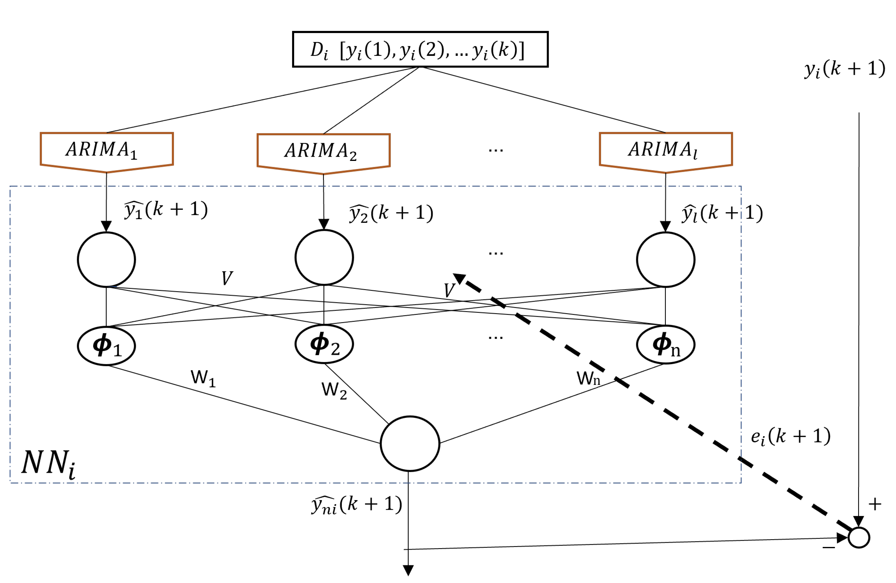
We use back-propagation algorithm to obtain

[V^{*}, W^{*}],

see Figure 4. Here

A R I M A_{j} (D_{j})

is trained by its own data set

D_{j}

as in Figure 1, then the neural network

N N_{i}

is trained by

D_{i}

, such that

{\hat{y}}_{n i} (k + 1)

from (21) is better than

{\hat{y}}_{i} (k + 1),

{\hat{y}}_{i} (k + 1) = A R I M A_{i} (D_{i})

(23)

Transfer Learning: Different datasets with their corresponding ARIMA models can improve each other’s accuracy via knowledge transfer within the neural network. The fusion scheme of different ARIMA models using a neural network is illustrated in Algorithm 2.

Algorithm 2 Fusion of ARIMA models using a neural network.

1:: Prepare datasets $D_{1}, D_{2}, . . . D_{l}$
2:: Use Algorithm 1 to obtain l ARIMA models $A R I M A_{1}, . . . A R I M A_{l}$
3:: The output of each ARIMA model serves as input to the neural network
4:: Use $D_{1}, D_{2}, . . . D_{l}$ again and backpropagation to train the fusion weights
5:: Return the fusion neural network

Algorithm Summary: (1) Train individual ARIMA models on separate datasets. (2) Feed outputs from each ARIMA model as input to the neural network. (3) Train the neural network using backpropagation to minimize prediction error.

3.4.2. Compensation Strategy

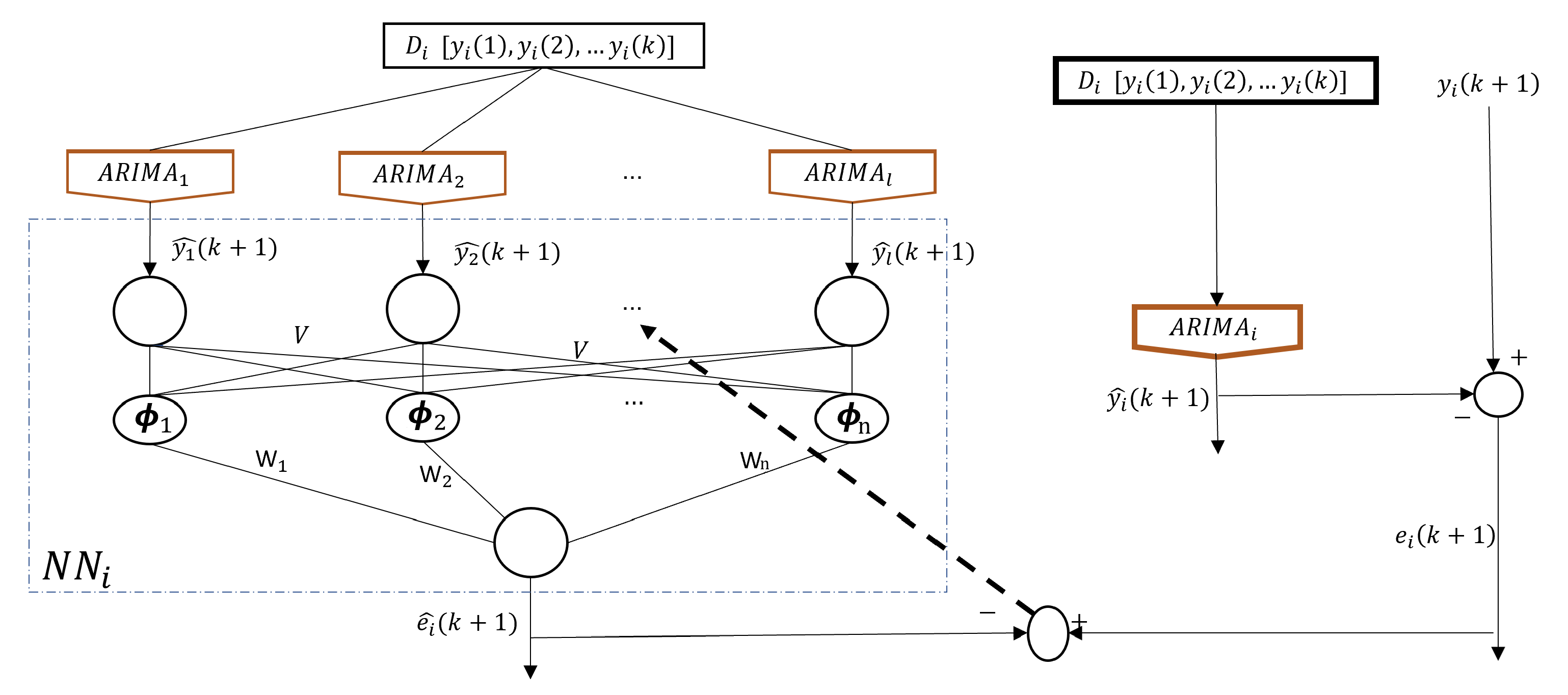
The network architectureis the same as in the fusion strategy. We use a neural network to learn the prediction error of ARIMA model, see Figure 5.

After the first step training as in Figure 1, the prediction error of ARIMA model is

e_{i} (k + 1) = y_{i}^{*} (k + 1) - A R I M A_{i} (D_{i})

The output of the multiple ARIMA models is the same as (21), but

A_{o} (k)

A_{o} (k) = A R I M A_{o} (D_{o}), o = 1 \dots l, o \neq i

The training objective is to minimize the difference between the prediction error of each ARIMA model and the neural network’s output,

{\hat{e}}_{i} (k + 1) = e_{i} (k + 1) - y_{n i} (k + 1)

The training error object is

[V^{*}, W^{*}] = arg min_{V, W} \sum {\hat{e}}_{i}^{2} (k + 1)

(24)

Error correction: The neural network learns the individual errors of each ARIMA model and corrects them, enhancing overall accuracy,

A R I M A_{i} (D_{i}) + {\hat{y}}_{n i} (k + 1) A R I M A_{i} (D_{i}) + {\hat{e}}_{i} (k + 1)

(25)

The training process of neural network compensation is shown in Algorithm 3.

Algorithm 3 Multiple ARIMA with neural network compensation.

1:: Prepare data sets $D_{1}, D_{2}, . . . D_{l}$
2:: Use Algorithm 1 to obtain l ARIMA models $A R I M A_{1}, . . . A R I M A_{l}$
3:: Calculate the modeling errors between $D_{1}, D_{2}, . . . D_{l}$ and neural networks
4:: Use the above modeling errors and back-propagation to train the neural netwwork
5:: Return the ARIMA model and neural network

Algorithm Summary: (1) Train individual ARIMA models on separate datasets. (2) Calculate the prediction error for each ARIMA model. (3) Train the neural network using combined prediction errors and backpropagation.

4. Experiments

4.1. Pre-Process of Wind Energy Data

In this section, we present the experimental results of our analysis on three different wind energy datasets from various locations around the world [29]:

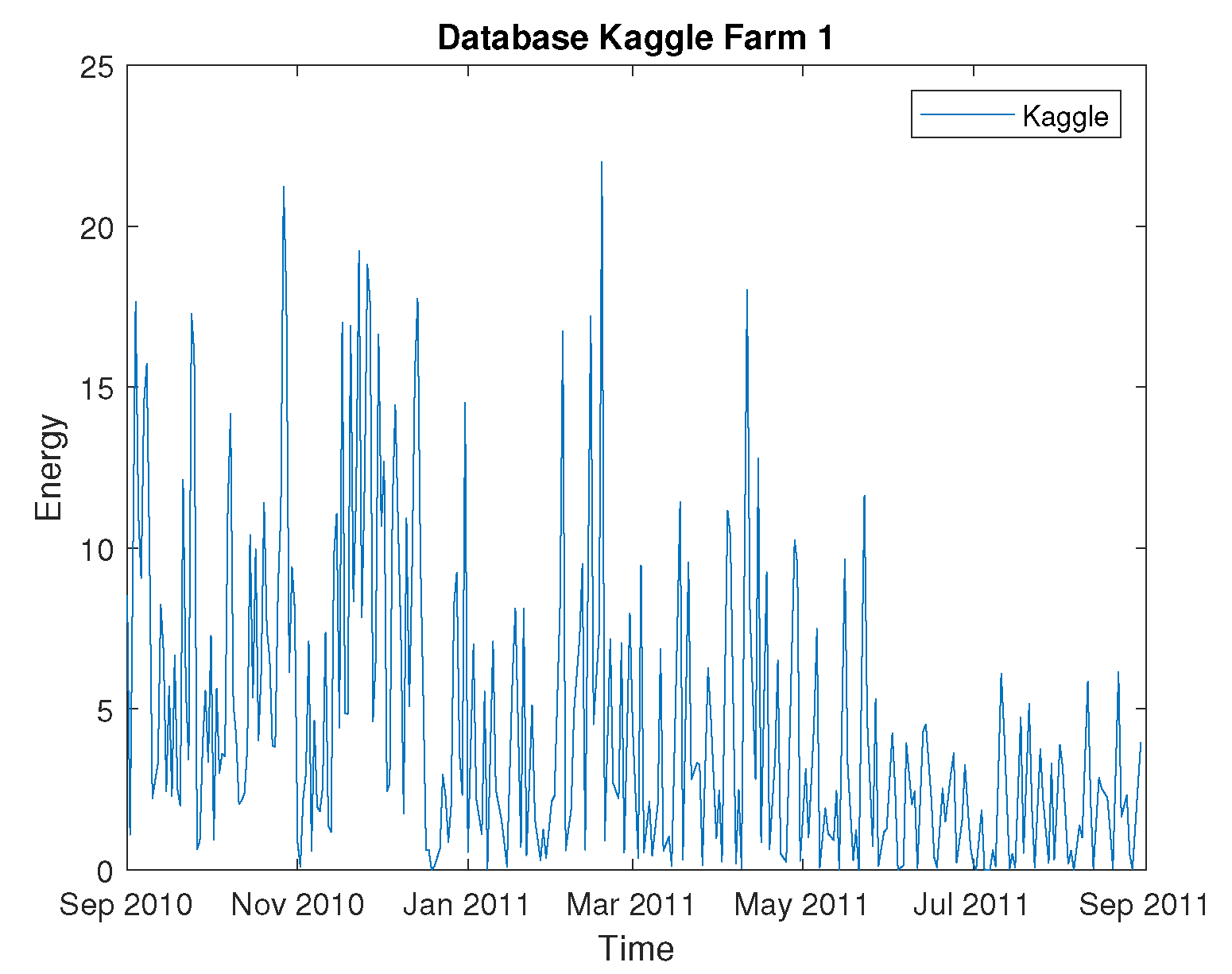
The Kaggle dataset contains hourly values from seven wind farms spanning from July 2009 to June 2012. We use data from the first wind farm between 1 July 2009, and 31 December 2010. To create a daily time series, we summarize 24 hours of data into one data point. The dataset contains 295 data points, of which 221 are used for training and 74 for testing.
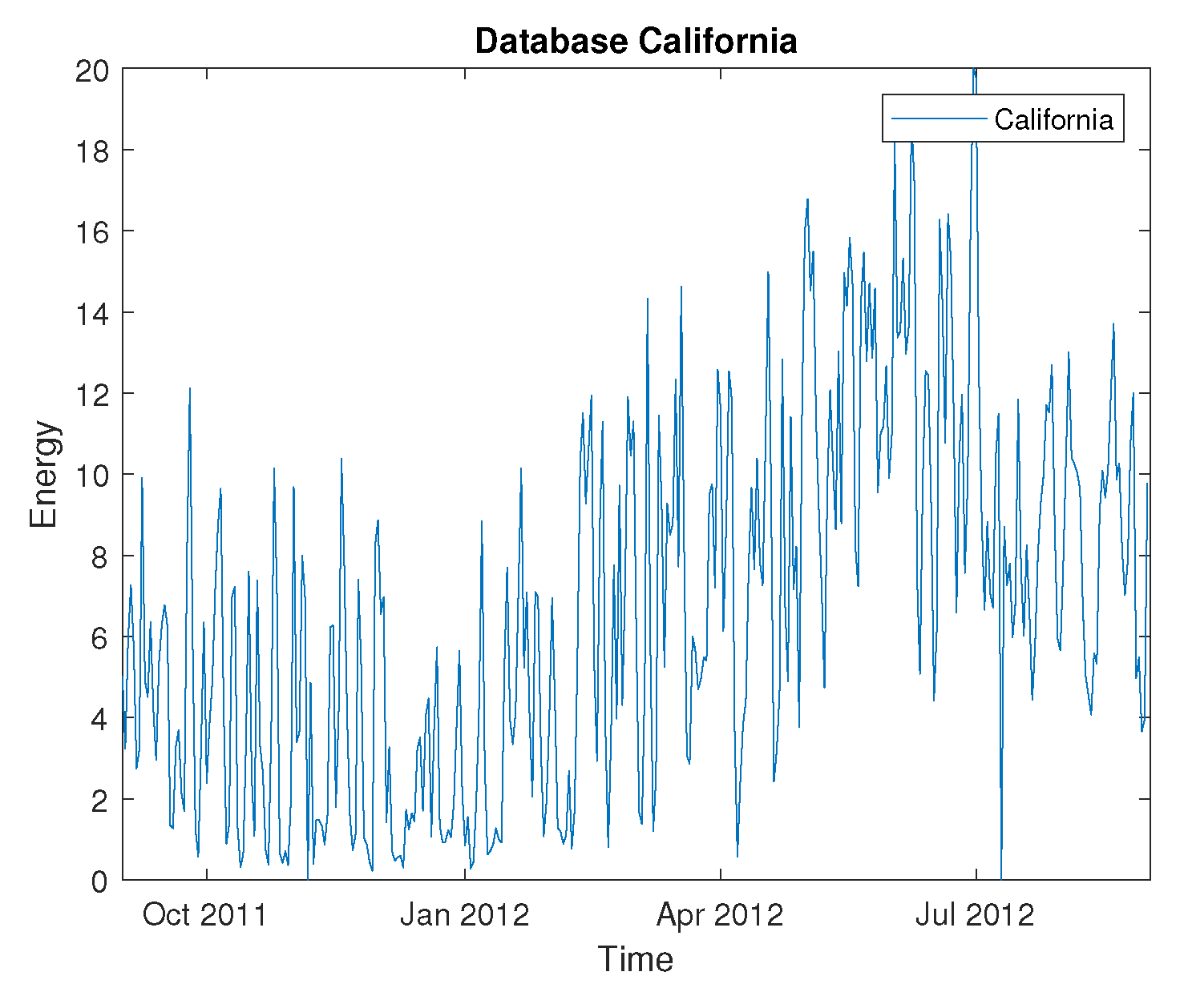
The California dataset records hourly energy production from various sources, including geothermal, biomass, biogas, mini-hydraulic, total wind, solar photovoltaic, and solar thermal. We use data from 1 September 2011, to 31 August 2012. Similar to the Kaggle dataset, we create a daily time series by summarizing 24 hours of data into one data point. The dataset contains 366 data points, of which 274 are used for training and 92 for testing.
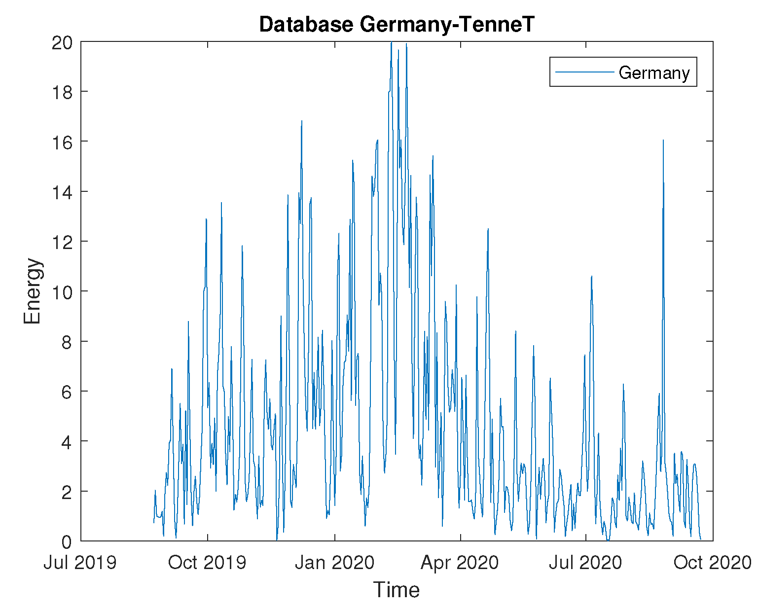
The Germany dataset records wind power measurements from four different wind farms: Tennet, 50Hertz, TransnetBW, and Amprion. The dataset records measurements every five minutes, resulting in 96 measurements per day. To create a daily time series, we summarize 96 measurements into one data point. The dataset contains 397 data points, of which 298 are used for training and 99 for testing.

We use

75 %

of the data for single ARIMA modeling and neural networks training, while the remaining

25 %

is used for testing. To avoid anomalies and redundancies, we normalize all datasets using the formula

x_{n o r m} (i) = \frac{x_{i} - m i n (x)}{m a x (x) - m i n (x)}

(26)

where

x_{i}

is each datum of the time series,

m i n (x)

is the minimum of the data

x,

and

m a x (x)

is the maximum of the data

x .

Figure 6, Figure 7 and Figure 8 display the normalized time series of the three datasets. The abscissa axis represents the days, while the ordinate axis represents wind energy in gigawatts.

4.2. Single ARIMA Modeling

The single ARIMA modeling needs two steps: structure determination and parameter identification, see Figure 1. Each single ARIMA model requires three structure parameters

(p, d, q)

p represents the order of the AR (auto-regression) term that uses past values in the regression equation (1) for the time series.
d represents the number of differentiations required for the time series to become stationary.
q represents the order of the MA (moving average) term that represents the model error as a combination of the above error terms as shown in the equation. For long-term prediction of time series, we use, $m > 0 .$

$y_{t + m} = y_{t} \sum_{k = 1}^{p} a_{i} z^{- k} + ϵ_{t} {(1 - z^{- 1})}^{- d} \sum_{k = 1}^{q} b_{j} z^{- k} + ϵ_{t} {(1 - z^{- 1})}^{- d}$

where $y_{t}$ represents the time series, $ϵ_{t}$ is white noise. In this paper, we regard it as the model error. For short-term forcating, $m = 0 .$ In this paper, we use thrre steps prediction, $m = 2 .$

To determine the structure of the ARIMA model

(p, d, q)

, we first need to analyze the stationary properties and obtain the parameter d. We use the augmented Dickey-Fuller method (ADF). The results of the stationary tests are shown in Table 1.

Next, we calculate the

(p, q)

values using the autocorrelation function, ACF/PAF. The critical values for ADF hypothesis are

1 %

5 %

and

10 %

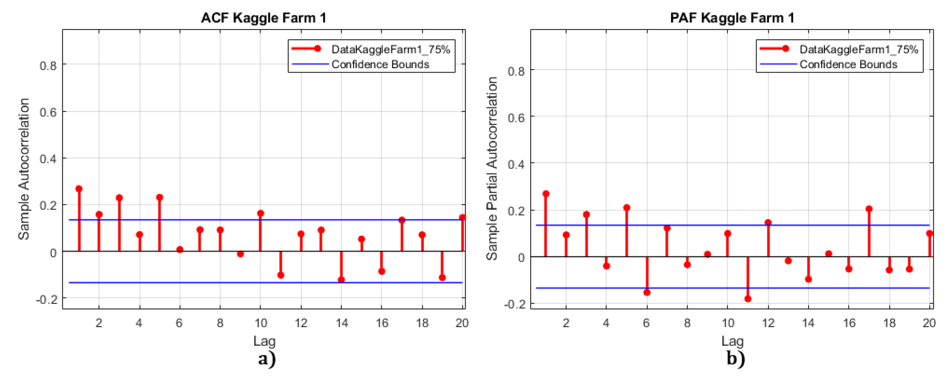
. These values are used to determine if the ARIMA model has a unit root, and if the series is non-stationary. ACF/PAF analysis for the three datasets is shown in Figure 9, Figure 10 and Figure 11.

For the Kaggle dataset, the first ADF test with zero differentiation has a value of $- 2.153$ . This value is less than all critical values, indicating that the time series needs to be differentiated. After one differentiation, the hypothesis is accepted and the series becomes stationary with $d = 1$ . Figure 9 shows the ACF analysis of the Kaggle dataset, which identifies possible candidates for the q parameter as $1, 2, 3, 4, 5$ , and 6.The PAF analysis of the Kaggle dataset identifies possible candidates for the p parameter as $1, 2, 3$ , and 4.
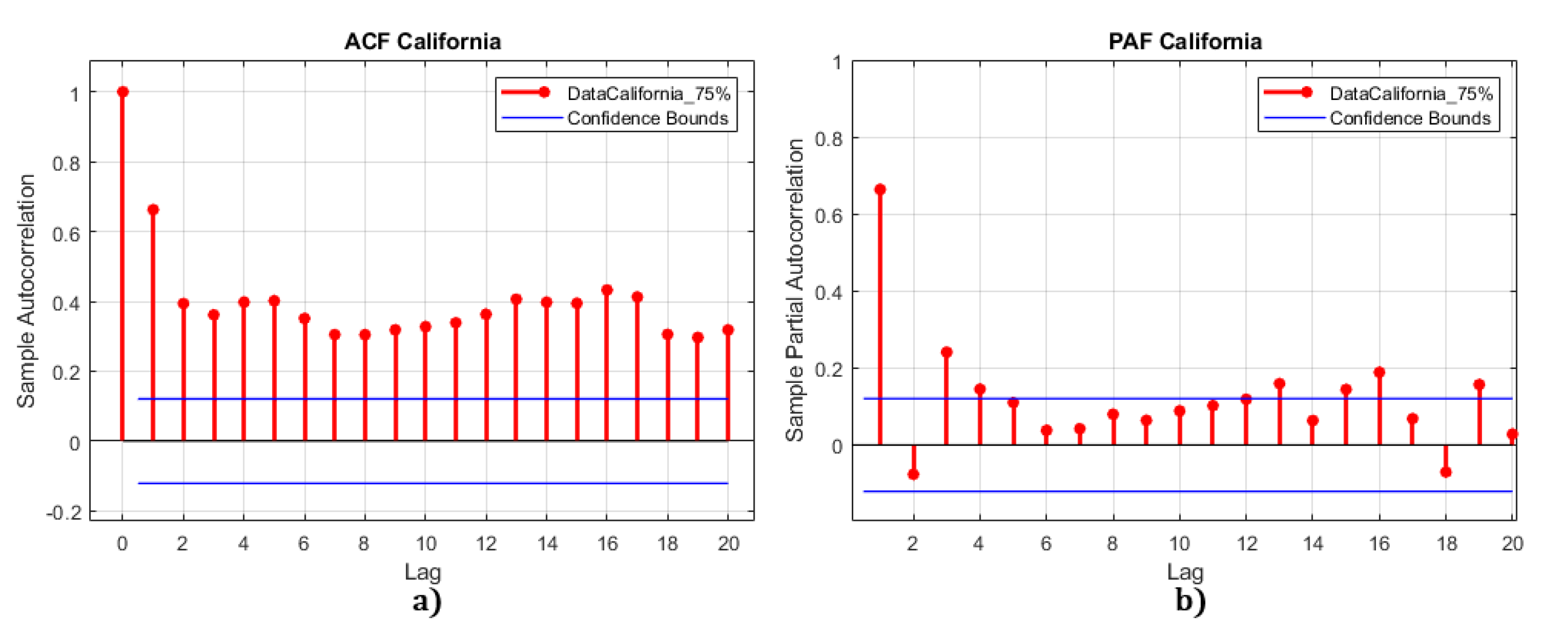
For the California dataset, the first ADF test has a value of $- 1.22$ , which is less than all critical values. After one differentiation, the series becomes stationary with $d = 1$ . Similarly, Figure 10 shows the ACF analysis of the California dataset, which identifies possible candidates for the q parameter as $1, 2$ , and 3, the PAF analysis of the California dataset identifies possible candidates for the p parameter as $1, 2$ , and 4.
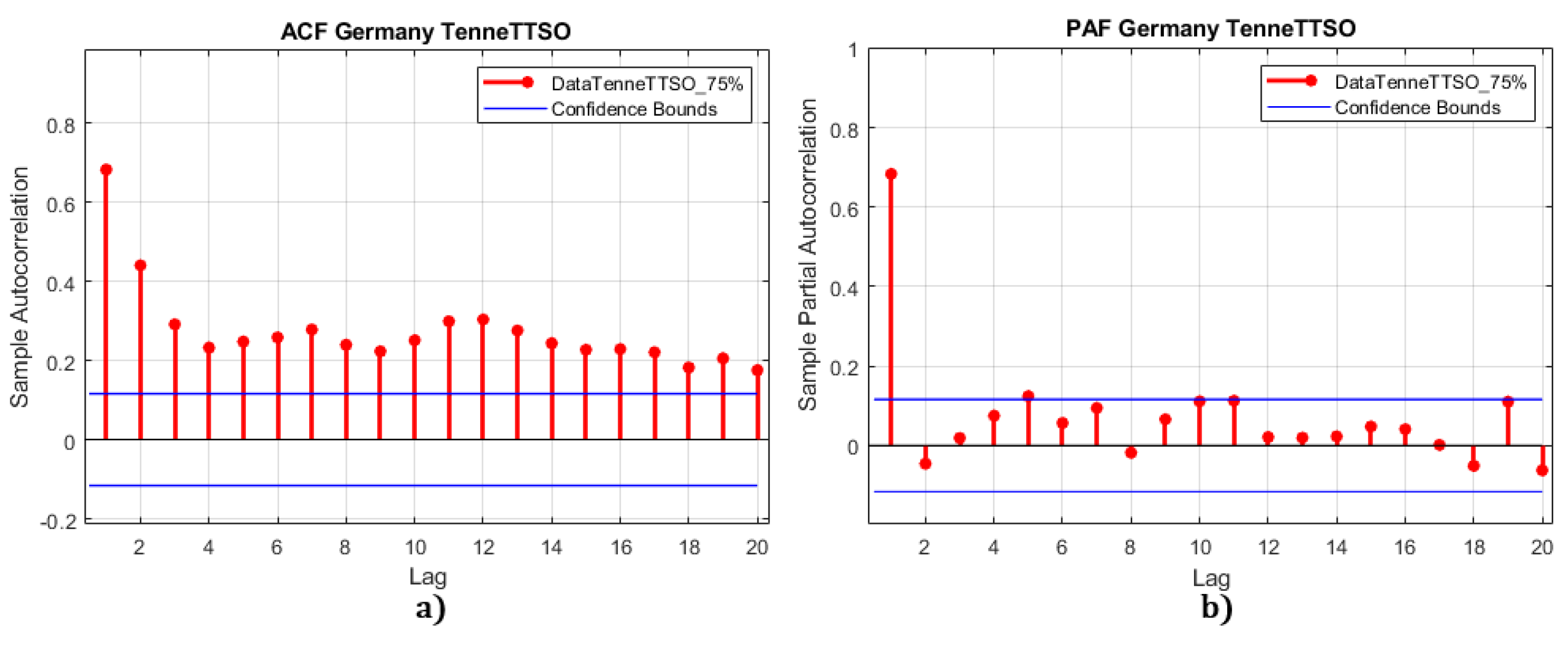
For the Germany dataset, the first ADF value is $- 2.898$ . The critical value $1 %$ is not valid, as it is greater than the other critical values ( $5 %$ and $10 %$ ). Therefore, the series is almost stationary with $d = 0$ . For Figure 11, the ACF analysis of the Germany dataset identifies possible candidates for the q parameter as $1, 2, 3, 4$ , and 5, the PAF analysis of the Germany dataset identifies possible candidates for the p parameter as 1 and 2.

Finally, the structure parameters of the three ARIMA models are summarized in Table 2.

The next step is to use the AIC (Akaike Information Criterion) criterion (9) to obtain the best ARIMA model. he best ARIMA model. The lower the AIC, the better the model. If two models have the same amount of variance, the one with fewer parameters will have a lower AIC and will be the best fit model. Table 3 presents the AIC values for different

(p, d, q)

combinations. Therefore, the best ARIMA model for the Kaggle dataset is

A R I M A (1, 1, 2)

, for the Germany dataset is

A R I M A (1, 0, 4)

, and for the California dataset is

A R I M A (0, 1, 2)

4.3. Multiple ARIMA Models Training

A fundamental requirement of transfer learning is for a larger domain

Λ_{a}

to transfer features to a smaller domain

Λ_{b}

. In our case, we have trained ARIMA models on three datasets as mentioned, and these pre-trained models will represent our domain

Λ_{a}

. The domain

Λ_{b}

will depend on the dataset to be evaluated, such as California, Kaggle, or Germany, and when a dataset is selected, it will be evaluated on all three pre-trained models. As discussed above, the outputs of these models will serve as inputs for our neural network, allowing us to train and optimize its weights using backpropagation to achieve fusion of the features.

However, it should be noted that the training samples are small, i.e., less than 300, and a single ARIMA model alone may not provide accurate prediction results. For the three datasets, the input data are denoted as

D_{i}

, where

i = \{C a l i f o r n i a, G e r m a n y, K a g g l e\}

. The trained single ARIMA models are represented as

A R I M A_{i,}

and the output of the ARIMA model is

y_{i} (k + 1) .

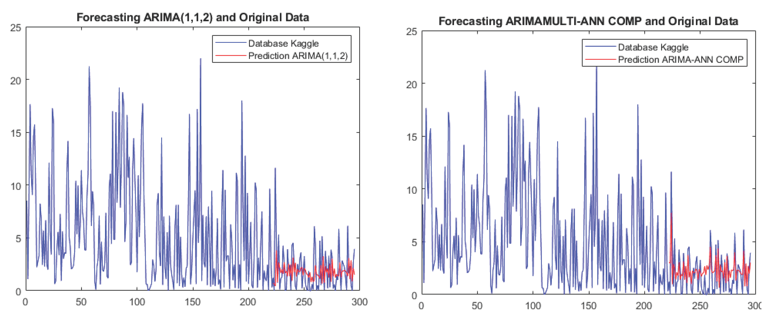
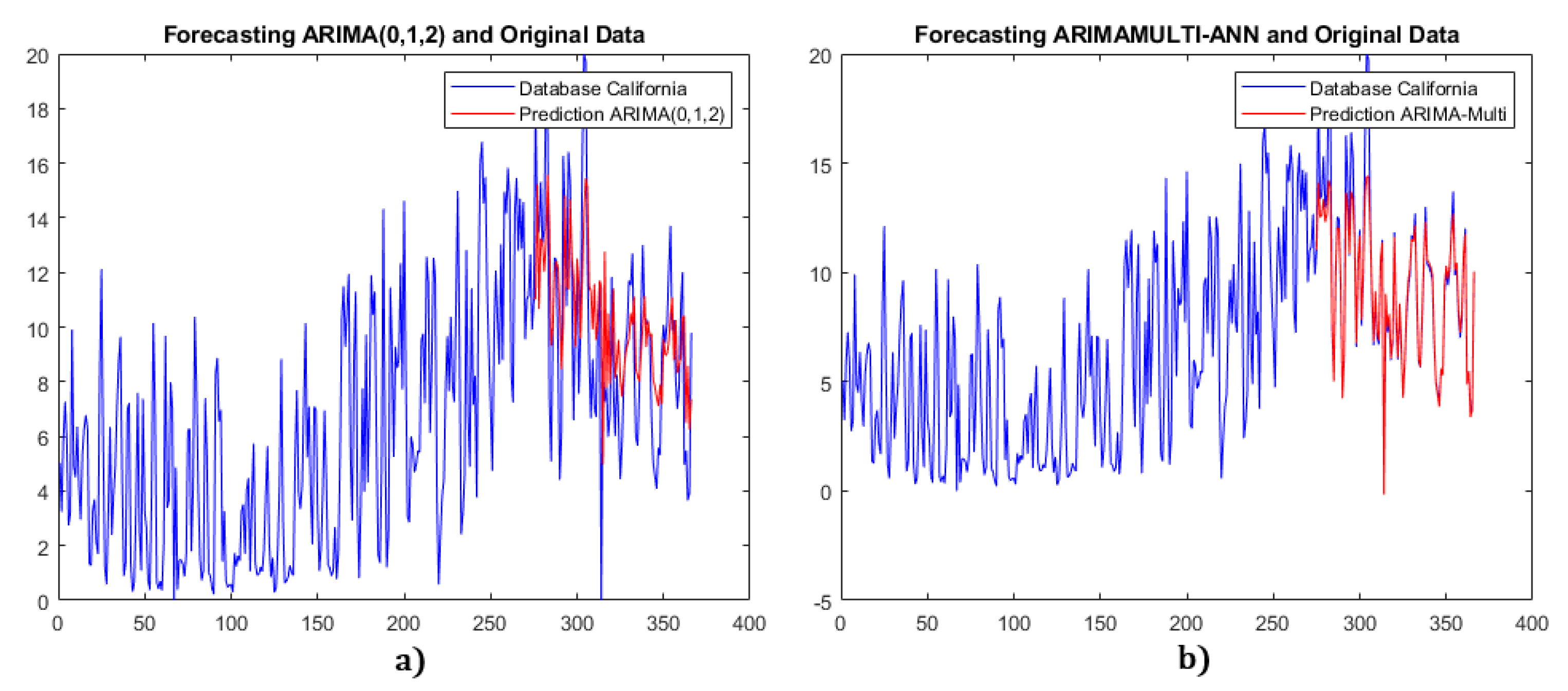
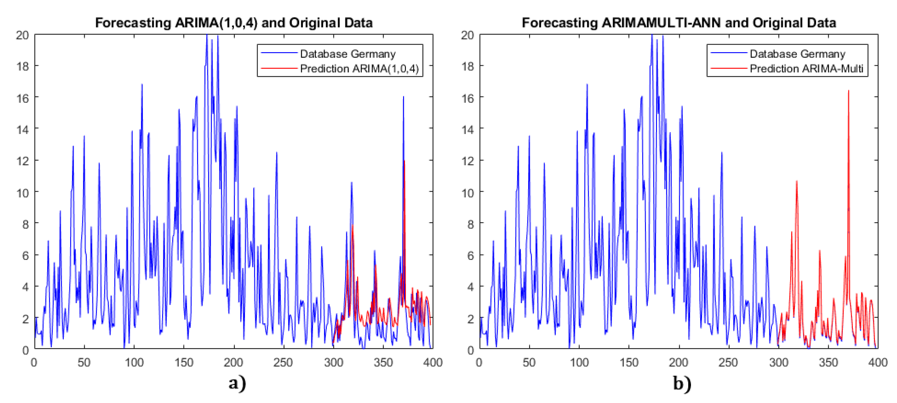
For the California and Germany datasets, we use the neural network fusion method for multiple ARIMA models, while for the Kaggle dataset, we use neural network compensation. Figure 12, Figure 13 and Figure 14 show the comparison results between the single ARIMA and multiple ARIMA with neural network fusion.

4.4. Comparison Results

The forecasting errors of the three datasets are shown in Table 4, Table 5 and Table 6, where the mean absolute error (MAE), symmetric mean absolute percentage error (SMAPE), root mean squared error (RMSE), and R-squared (RSQ) are defined as,

\begin{matrix} M A E = \frac{\sum_{i}^{n} |y_{i}^{*} - y_{i}|}{n} \\ S M A P E = \frac{1}{n} \sum_{i}^{n} \frac{|y_{i}^{*} - y_{i}|}{(y_{i}^{*} - y_{i}) / 2} \\ R M S E = \sqrt{\frac{\sum_{i}^{n} {(y_{i}^{*} - y_{i})}^{2}}{n}} \\ R S Q = 1 - \frac{\sum_{i}^{n} {(y_{i}^{*} - y_{i})}^{2}}{\sum_{i}^{n} {(y_{i}^{*} - \bar{y})}^{2}}, \bar{y} = \frac{1}{n} \sum_{i}^{n} y_{i} \end{matrix}

For the California data, each metric of the multiple ARIMA model has at least a

50 %

reduction compared to the single ARIMA model. For instance, the MAE metric shows an improvement of

74.37 %

. Similarly, for the Germany dataset, the multiple ARIMA model outperforms the single ARIMA model, with an average improvement of

89 %

. For the Kaggle dataset, the average improvement in SMAPE, RMSE, and RSQ metrics is

35.68 %

. These results demonstrate that the forecasting accuracies of the proposed multiple ARIMA models are better than those of the single ARIMA models.

Furthermore, we observe that the multiple ARIMA model for the Germany dataset has an average improvement of almost

90 %

over the single

A R I M A (1, 0, 4)

model, whereas for the California dataset, there is an improvement of approximately

65 %

, and for the Kaggle dataset, the improvement is around

35 %

. Finally, we performed iteration tests to verify the stability of the proposed models. We ran 1000 repetitions for each multiple ARIMA model, stored the errors, and calculated the average. The results showed a change of less than

1 %

in each set, demonstrating that the proposed models are stable and reliable.

In summary, the comparative tables indicate that the prediction errors are significantly lower with the proposed multiple ARIMA models than with the single ARIMA models. The MAE, SMAPE, and RMSE metrics are notably reduced, while the RSQ metric is closer to 1 in the proposed models compared to the single ARIMA models. RSQ is much better when the “ARIMA model with NN fusion” is used.

5. Conclusions

We introduce an innovative time series forecasting method designed to tackle the challenges associated with missing data, a common occurrence in wind energy systems. Our approach integrates multiple ARIMA models through neural network learning. The combination of these multiple ARIMA models incorporates two mechanisms: the fusion of diverse models and compensation derived from the others. Leveraging the strengths of both neural networks and ARIMA models, we apply our methods to wind energy systems, resulting in a significant improvement in prediction accuracy across three benchmark datasets: Germany, California, and Kaggle. Our focus will center on conducting experiments and validations to compare various models, including statistical, AI-based, and hybrid models. Additionally, we aim to study and test physical variables to analyze the behavior of the proposed model.

References

Yatiyana, E.; Rajakaruna, S.; Ghosh, A. Wind speed and direction forecasting for wind power generation using ARIMA model. In Proceedings of the 2017 Australasian Universities Power Engineering Conference (AUPEC), 2017; pp. 1–6. [Google Scholar] [CrossRef]
Yunus, K.; Thiringer, T.; Chen, P. ARIMA-Based Frequency-Decomposed Modeling of Wind Speed Time Series. Transactions on Power Systems 2016, 31, 977–990. [Google Scholar] [CrossRef]
Elsaraiti, M.; Merabet, A.; Al-Durra, A. Time Series Analysis and Forecasting of Wind Speed Data. In Proceedings of the 2019 IEEE Industry Applications Society Annual Meeting, 2019; pp. 1–5. [Google Scholar] [CrossRef]
Eldali, F.A.; Hansen, T.M.; Suryanarayanan, S.; Chong, E.K.P. Employing ARIMA models to improve wind power forecasts: A case study in ERCOT. In Proceedings of the 2016 North American Power Symposium (NAPS), 2016; pp. 1–6. [Google Scholar] [CrossRef]
Zhang, Y.; Zhao, Y. Research on Wind Power Prediction Based on Time Series. In Proceedings of the 2021 IEEE International Conference on Artificial Intelligence and Industrial Design (AIID), 2021; pp. 78–82. [Google Scholar] [CrossRef]
Maya, M.; Yu, W.; Li, X. Time series forecasting with missing data using neural network and meta-transfer learning. In Proceedings of the 2021 IEEE Symposium Series on Computational Intelligence (SSCI 2021), 2021; pp. 1–6. [Google Scholar] [CrossRef]
Lu, P.; Ye, L.; Tang, Y.; Zhao, Y.; Zhong, W.; Qu, Y.; Zhai, B. Ultra-short-term combined prediction approach based on kernel function switch mechanism. Renewable Energy 2021, 164, 842–866. [Google Scholar] [CrossRef]
Aasim; Singh, S.N.; Mohapatra, A. Repeated wavelet transform based ARIMA model for very short-term wind speed forecasting. Renewable Energy 2019, 136, 758–768. [Google Scholar] [CrossRef]
Zhang, L.; Zhang, D. Domain Adaptation Extreme Learning Machines for Drift Compensation in E-Nose Systems. IEEE Transactions on Instrumentation and Measurement 2015, 64, 1790–1801. [Google Scholar] [CrossRef]
Ye, R.; Dai, Q. A novel transfer learning framework for time series forecasting. Knowledge-Based Systems 2018, 156, 74–99. [Google Scholar] [CrossRef]
Long short-term memory neural network for traffic speed prediction using remote microwave sensor data. Transportation Research Part C: Emerging Technologies 2015, 54, 187–197. [CrossRef]
Pasari, S.; Shah, A.; Sirpurkar, U. Wind Energy Prediction Using Artificial Neural Networks. In Enhancing Future Skills and Entrepreneurship; Springer International Publishing, 2020; pp. 101–107. [Google Scholar] [CrossRef]
Navas, R.K.B.; Prakash, S.; Sasipraba, T. Artificial Neural Network based computing model for wind speed prediction: A case study of Coimbatore, Tamil Nadu, India. Physica A: Statistical Mechanics and its Applications 2020, 542, 123–383. [Google Scholar] [CrossRef]
Ahadi, A.; Liang, X. Wind Speed Time Series Predicted by Neural Network. In Proceedings of the 2018 IEEE Canadian Conference on Electrical Computer Engineering (CCECE); 2018; pp. 1–4. [Google Scholar] [CrossRef]
Madhiarasan, M. Accurate prediction of different forecast horizons wind speed using a recursive radial basis function neural network. Protection and Control of Modern Power Systems 2020, 5, 22. [Google Scholar] [CrossRef]
Liu, F.; Li, R.; Dreglea, A. Wind Speed and Power Ultra Short-Term Robust Forecasting Based on Takagi–Sugeno Fuzzy Model. Energies 2019, 12. [Google Scholar] [CrossRef]
Dhunny, A.; Doorga, J.; Allam, Z.; Lollchund, M.; Boojhawon, R. Identification of optimal wind, solar and hybrid wind-solar farming sites using fuzzy logic modelling. Energy 2019, 188, 116056. [Google Scholar] [CrossRef]
Shabbir, N.; AhmadiAhangar, R.; Katt, L.; Iqbal, M.N.; Rosin, A. Forecasting Short Term Wind Energy Generation using Machine Learning. In Proceedings of the 2019 IEEE 60th International Scientific Conference on Power and Electrical Engineering of Riga Technical University (RTUCON); 2019; pp. 1–4. [Google Scholar] [CrossRef]
Tian, Z.; Chen, H. Multi-step short-term wind speed prediction based on integrated multi-model fusion. Applied Energy 2021, 298, 117248. [Google Scholar] [CrossRef]
Liu, H.; Tian, H.Q.; Li, Y.F.; Zhang, L. Comparison of four Adaboost algorithm based artificial neural networks in wind speed predictions. Energy Conversion and Management 2015, 92, 67–81. [Google Scholar] [CrossRef]
Greff, K.; Srivastava, R.K.; Koutník, J.; Steunebrink, B.R.; Schmidhuber, J. LSTM: A Search Space Odyssey. IEEE Transactions on Neural Networks and Learning Systems 2017, 28, 2222–2232. [Google Scholar] [CrossRef] [PubMed]
Aasim; Singh, S.; Mohapatra, A. Repeated wavelet transform based ARIMA model for very short-term wind speed forecasting. Renewable Energy 2019, 136, 758–768. [Google Scholar] [CrossRef]
Gupta, A.; Kumar, A.; Boopathi, K. Intraday wind power forecasting employing feedback mechanism. Electric Power Systems Research 2021, 201, 107518. [Google Scholar] [CrossRef]
Liu, H.; Tian, H.Q.; Li, Y.F. Comparison of two new ARIMA-ANN and ARIMA-Kalman hybrid methods for wind speed prediction. Applied Energy 2012, 98, 415–424. [Google Scholar] [CrossRef]
Ye, R.; Suganthan, P.N.; Srikanth, N.; Sarkar, S. A hybrid ARIMA-DENFIS method for wind speed forecasting. In Proceedings of the 2013 IEEE International Conference on Fuzzy Systems (FUZZ-IEEE), 2013; pp. 1–6. [Google Scholar] [CrossRef]
Abbasipour, M.; Igder, M.A.; Liang, X. A Novel Hybrid Neural Network-Based Day-Ahead Wind Speed Forecasting Technique. IEEE Access 2021, 9, 151142–151154. [Google Scholar] [CrossRef]
Aly, H.H. An intelligent hybrid model of neuro Wavelet, time series and Recurrent Kalman Filter for wind speed forecasting. Sustainable Energy Technologies and Assessments 2020, 41, 100802. [Google Scholar] [CrossRef]
Li, X.; Sabas, F.; Duarte, V. Wind energy forecasting using multiple ARIMA models. In Proceedings of the 2022 IEEE 18th International Conference on Automation Science and Engineering (CASE), 2022; pp. 2034–2039. [Google Scholar] [CrossRef]
Khashei, M.; Bijari, M. An artificial neural network (p,d,q) model for timeseries forecasting. Expert Systems with Applications 2010, 37, 479–489. [Google Scholar] [CrossRef]
Wang, L.; Zou, H.; Su, J.; Li, L.; Chaudhry, S. An ARIMA-ANN hybrid model for time series forecasting. Systems Research and Behavioral Science 2013, 30. [Google Scholar] [CrossRef]
Aahin, A.A.; Ertekin, A. Improving forecasting accuracy of time series data using a new ARIMA-ANN hybrid method and empirical mode decomposition. Neurocomputing 2019, 361, 151–163. [Google Scholar] [CrossRef]

Figure 1. Single ARIMA model for time series forecasting

Figure 2. Classical combination method of ARIMA and neural networks

Figure 3. The proposed two integration methods between ARIMA and neural networks

Figure 4. Training for fusion strategy

Figure 5. Ttraining for compensation strategy.

Figure 6. California wind energy dataset.

Figure 7. Tennet wind energy dataset.

Figure 8. Kaggle wind energy dataset.

Figure 9. ACF/PAF analysis of the Kaggle data set

Figure 10. ACF/PAF analysis of the California data set.

Figure 11. ACF/PAF analysis of the Germany data set.

Figure 12. (a) Single ARIMA

(1, 0, 4)

for California data. (b) Multiple ARIMA model with NN fusion.

Figure 12. (a) Single ARIMA

(1, 0, 4)

for California data. (b) Multiple ARIMA model with NN fusion.

Figure 13. (a) Single ARIMA

(0, 1, 4)

for Germany data. (b) Multiple ARIMA model with NN fusion.

Figure 13. (a) Single ARIMA

(0, 1, 4)

for Germany data. (b) Multiple ARIMA model with NN fusion.

Figure 14. (a) Single ARIMA

(1, 1, 2)

for Kaggle data. (b) Multiple ARIMA model with NN compensation.

Figure 14. (a) Single ARIMA

(1, 1, 2)

for Kaggle data. (b) Multiple ARIMA model with NN compensation.

Table 1. Dickey-Fuller testing results of the data sets.

Serie	ADF Statistic	p-Value	1%	5%	10%	H0	d
Kaggle	−2.153723606	0.22346750	−3.449	−2.870	−2.571	not stationary	0
Kaggle	−7.903060508	4.1355332e-12	−3.449	−2.870	−2.571	stationary	1
Germany	−2.8986826	0.0455013	−3.447	−2.869	−2.569	stationary	0
California	−1.226807	0.661958	−3.449	−2.870	−2.571	not stationary	0
California	−9.737932	8.649381e-17	−3.449	−2.870	−2.571	stationary	1

Table 2. ARIMA parameters obtained with the tests of ACF, PAF and the augmented Dickey-Fuller test.

Serie	p	d	q
Germany	1,2	0	1,2,3,4,5
California	1,2,3,4,5,6	1	0
Kaggle	1,2	1	1,2,3

Table 3. ARIMA models with AIC criteria.

Germany[Tennet]		California		Kaggle[FARM 1]
Model	AIC	Model	AIC	Model	AIC
ARIMA(1,0,4)	1544.3	ARIMA(0,1,2)	1367.3	ARIMA(1,1,2)	1336.2
ARIMA(1,1,4)	1544.8	ARIMA(0,1,3)	1368.5	ARIMA(2,1,1)	1337.1
ARIMA(2,0,5)	1545.0	ARIMA(1,1,2)	1368.8	ARIMA(2,1,3)	1337.8
ARIMA(1,1,2)	1546.7	ARIMA(0,1,4)	1369.2	ARIMA(1,1,3)	1338.2
ARIMA(2,1,3)	1546.9	ARIMA(1,1,3)	1369.7	ARIMA(2,1,2)	1338.3
ARIMA(1,1,3)	1547.0	ARIMA(1,1,4)	1371.2	ARIMA(1,1,1)	1340.1
ARIMA(2,0,2)	1554.3	ARIMA(2,1,3)	1371.3
ARIMA(1,0,2)	1554.8	ARIMA(6,1,2)	1376.4

Table 4. Comparison of forecasting errors with California data.

Model	MAE	SMAPE	RMSE	RSQ
ARIMA(0,1,2) California	2.4117	0.2676	3.139	0.3428
ARIMA-Multi California	0.6181	0.0715	1.263	0.8934

Table 5. Comparison of forecasting errors with Germany data

Model	MAE	SMAPE	RMSE	RSQ
ARIMA(1,0,4) Germany	1.4644	0.6931	2.1952	0.1435
ARIMA-Multi Germany	0.0687	0.1239	0.0811	0.9988

Table 6. Comparison of forecasting errors with Kaggle data

Model	MAE	SMAPE	RMSE	RSQ
ARIMA-Multi Kaggle compensated	1.2064	0.8582	1.435	0.5322
ARIMA-Multi Kaggle	1.8351	0.9369	2.1223	-0.0231
ARIMA(1,1,2) Kaggle	1.6051	0.9938	2.2486	-0.1485

Disclaimer/Publisher’s Note: The statements, opinions and data contained in all publications are solely those of the individual author(s) and contributor(s) and not of MDPI and/or the editor(s). MDPI and/or the editor(s) disclaim responsibility for any injury to people or property resulting from any ideas, methods, instructions or products referred to in the content.

© 2024 by the author. Licensee MDPI, Basel, Switzerland. This article is an open access article distributed under the terms and conditions of the Creative Commons Attribution (CC BY) license (http://creativecommons.org/licenses/by/4.0/).

Copyright: This open access article is published under a Creative Commons CC BY 4.0 license, which permit the free download, distribution, and reuse, provided that the author and preprint are cited in any reuse.

MDPI Initiatives

Important Links

Choose an area of interest and we will send you notifications of new preprints at your preferred frequency.

Disclaimer

Time Series Forecasting with Missing Values Using Multiple Models: An Application to Wind Energy Systems

Abstract

1. Introduction

2. Single Linear Model for Time Series Forecasting Using Noise Estimation

2.1. ARIMA Linear Model

2.2. Structure of the Linear Model

2.3. Time Series Forecasting Using Noise Estimation

3. Multiple ARIMA Models with Neural Networks

3.1. Limitations of ARIMA and the Other Approaches

3.2. Multiple ARIMA Models

3.2.1. Transfer Learning for Robust ARIMA Models

3.2.2. Generalizing to Multiple Models

3.3. Combining ARIMA and Neural Networks for Enhanced Forecasting

3.4. Neural Network Training for ARIMA Combination and Correction

3.4.1. Fusion Strategy

3.4.2. Compensation Strategy

4. Experiments

4.1. Pre-Process of Wind Energy Data

4.2. Single ARIMA Modeling

4.3. Multiple ARIMA Models Training

4.4. Comparison Results

5. Conclusions

References

MDPI Initiatives

Important Links

Subscribe