Submitted:
29 February 2024
Posted:
29 February 2024
You are already at the latest version
Abstract
Keywords:
1. Introduction
2. Ground Reaction Force Estimation Methods
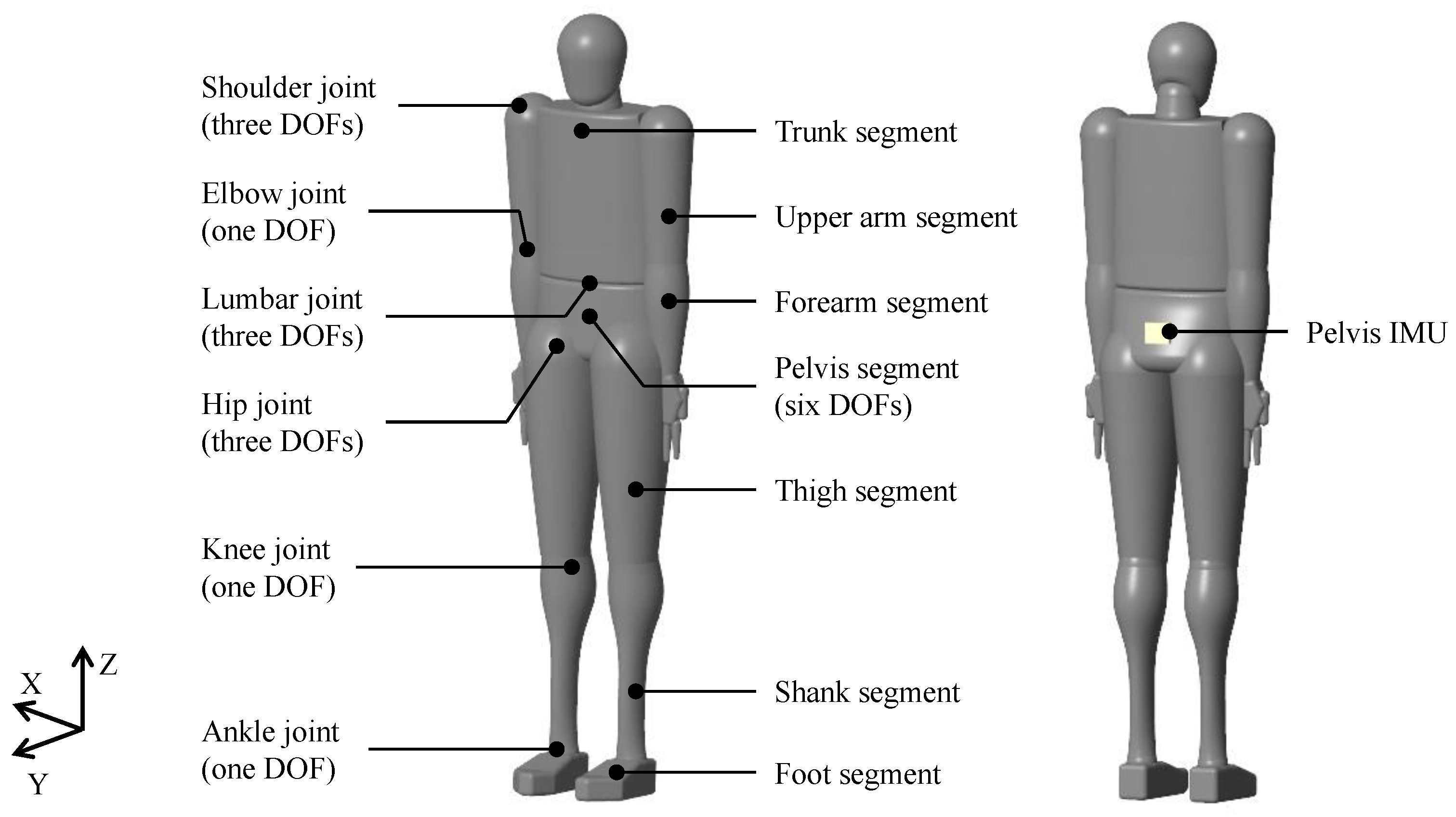
- The height and weight are input into the system, and a human model is constructed based on the inertia parameters calculated from them.
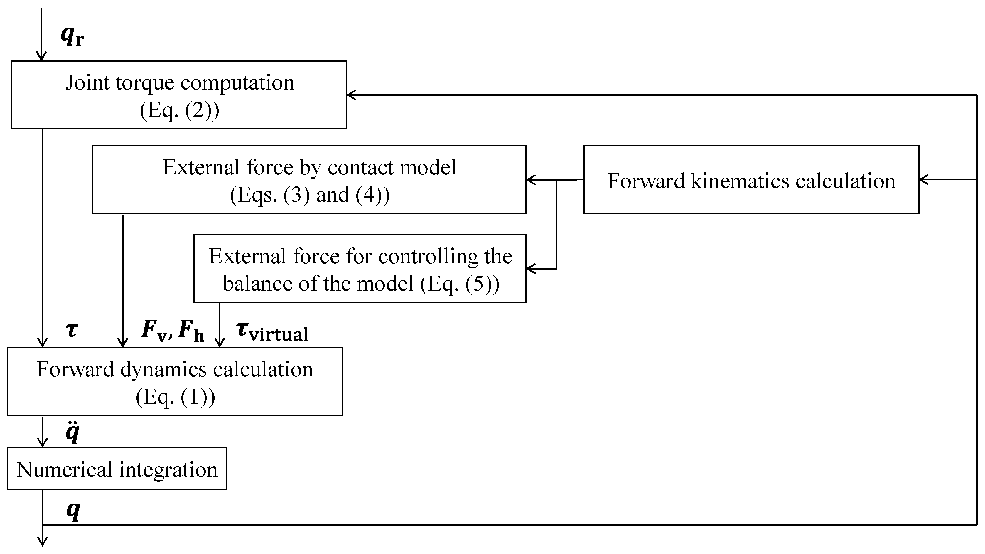
- Based on the reference joint angles formed by the node points, the forward dynamics model generates body movements.
- The body movement is evaluated by a cost function comprising errors between the generated body movement and measurements from IMUs, as well as internal biomechanical loads.
- Steps 2 and 3 are repeated while adjusting the node points of the reference joint angles to minimize the value of the cost function.
- Estimate GRFs, GRMs, and joint motion using the optimized node points in the forward dynamics model.
2.1. Forward Dynamics Model
2.1.1. Human Model
2.1.2. Joint Torque Model
2.1.3. External Force Model
2.2. Optimization Calculation
2.2.1. Orientation Estimation
3. Experiment
3.1. Participants
3.2. Conditions
3.3. Measurements
3.4. Data Analysis
4. Results
5. Discussion
5.1. Advantages of the Proposed Approach
5.2. Accuracy
5.3. Limitations
6. Conclusions
Author Contributions
Funding
Institutional Review Board Statement
Informed Consent Statement
Acknowledgments
Conflicts of Interest
References
- Luhtanen, P.; Komi, P.V. Mechanical power and segmental contribution to force impulses in long jump take-off. European Journal of Applied Physiology and Occupational Physiology 1979, 41, 267–274. [Google Scholar] [CrossRef]
- Barker, L.A.; Harry, J.R.; Mercer, J.A. Relationships between countermovement jump ground reaction forces and jump height, reactive strength index, and jump time. Journal of Strength and Conditioning Research 2018, 32, 248–254. [Google Scholar] [CrossRef]
- Le, P.A.; Maton, B. Initiation of a vertical jump: the human body's upward propulsion depends on control of forward equilibrium. Neuroscience Letters 2002, 323, 183–186. [Google Scholar] [CrossRef]
- Glazier, P.S. Beyond animated skeletons: How can biomechanical feedback be used to enhance sports performance? Journal of Biomechanics 2021, 129, 110686. [Google Scholar] [CrossRef] [PubMed]
- Bulat, M.; Korkmaz, C.N.; Arslan, Y.Z.; Herzog, W. Musculoskeletal simulation tools for understanding mechanisms of lower-limb sports injuries. Current Sports Medicine Reports 2019, 18, 210–216. [Google Scholar] [CrossRef]
- Low, D.C.; Dixon, S.J. Footscan pressure insoles: accuracy and reliability of force and pressure measurements in running. Gait Posture 2010, 32, 664–666. [Google Scholar] [CrossRef]
- Ancillao, A.; Tedesco, S.; Barton, J.; O’ Flynn, B. Indirect measurement of ground reaction forces and moments by means of wearable inertial measurement units: A systematic review. Sensors 2018, 18, 2564. [Google Scholar] [CrossRef] [PubMed]
- Allen, T.; Shepherd, J.; Wood, J.; Tyler, D.; Duncan, O. Chapter 16 - Wearables for disabled and extreme sports. In Digital Health; Academic Press, 2021; pp. 253–273. [Google Scholar] [CrossRef]
- Karatsidis, A.; Bellusci, G.; Schepers, H.M.; de Zee, M.; Andersen, M.S.; Veltink, P.H. Estimation of ground reaction forces and moments during gait using only inertial motion capture. Sensors 2016, 17, 75. [Google Scholar] [CrossRef] [PubMed]
- Chaaban, C.R.; Berry, N.T.; Armitano-Lago, C.; Kiefer, A.W; Mazzoleni, M.J.; Padua, D.A. Combining inertial sensors and machine learning to predict vGRF and knee biomechanics during a double limb jump landing task. Sensors 2021, 21, 4383. [Google Scholar] [CrossRef]
- Karatsidis, A.; Jung, M.; Schepers, H.M.; Bellusci, G.; de Zee, M.; Veltink, P.H. Michael Skipper Andersen, Musculoskeletal model-based inverse dynamic analysis under ambulatory conditions using inertial motion capture. Medical Engineering & Physics 2019, 65, 68–77. [Google Scholar] [CrossRef]
- Haraguchi, N.; Hase, K. Prediction of ground reaction forces and moments and joint kinematics and kinetics by inertial measurement units using 3D forward dynamics model. Journal of Biomechanical Science and Engineering 2024, 19, 23–00130. [Google Scholar] [CrossRef]
- Drillis, R.; Contini, R.; Bluestein, M. Body segment parameter: A survey of measurement techniques. Artificial Limbs 1964, 8, 329–351. [Google Scholar]
- Ae, M.; Tang, H.; Yokoi, T. Estimation of inertia properties of the body segments in Japanese athletes. Society of Biomechanism Japan (in Japanease). 1992, 11, 23–33. [Google Scholar] [CrossRef]
- Davy, D. T.; Audu, M. L. A dynamic optimization technique for predicting muscle forces in the swing phase of gait. Journal of Biomechanics 1987, 20, 187–201. [Google Scholar] [CrossRef] [PubMed]
- Engin, A.E. On the biomechanics of the shoulder complex. Journal of Biomechanics 1980, 13, 575–581. [Google Scholar] [CrossRef]
- Engin, A.E.; Chen, S.M. Kinematics and passive resistive properties of human elbow complex. Journal of Biomechanical Engineering 1987, 109, 318–323. [Google Scholar] [CrossRef] [PubMed]
- Pope, M.H.; Wilder, D.G.; Matteri, R.E.; Frymoyer, J.W. Experimental measurements of vertebral motion underload. Orthopedic Clinics of North America 1977, 8, 155–167. [Google Scholar] [CrossRef] [PubMed]
- Ren, L.; Jones, R.K.; Howard, D. Whole body inverse dynamics over a complete gait cycle based only on measured kinematics. Journal of Biomechanics 2008, 41, 2750–2759. [Google Scholar] [CrossRef]
- 20. Seng, K-Y.; Peter, V-S.L.; Lam, P-M. Neck muscle strength across the sagittal and coronal planes: an isometric study. Clinical Biomechanics 2002, 17, 545–547. [CrossRef]
- Grabiner, M.D.; Jeziorowski, J.J.; Divekar, A.D. Isokinetic measurements of trunk extension and flexion performance collected with the biodex clinical data station. Journal of Orthopaedic & Sports Physical Therapy 1990, 11, 590–598. [Google Scholar] [CrossRef]
- Ng, J.K.; Richardson, C.A.; Parnianpour, M.; Kippers, V. EMG activity of trunk muscles and torque output during isometric axial rotation exertion: a comparison between back pain patients and matched controls. Journal of Orthopaedic Research 2002, 20, 112–121. [Google Scholar] [CrossRef]
- Lindsay, D.M.; Horton, J.F. Trunk rotation strength and endurance in healthy normal and elite male golfers with and without low back pain. North American journal of sports physical therapy 2006, 1, 80–89, PMC2953310. [Google Scholar]
- Smith, J.C.; Darden, G.F. Peak torque comparison between isam 9000 and biodex isokinetic devices. Int J Health Sci 20176, 4, 7–13. [Google Scholar]
- Meeteren, J.v.; Roebroeck, M.E.; Stam, H.J. Test-retest reliability in isokinetic muscle strength measurements of the shoulder. Journal of rehabilitation medicine 2002, 34. 91–95. [CrossRef]
- Jenp, Y.N.; Malanga, G.A.; Growney, E.S.; An, K.N. Activation of the rotator cuff in generating isometric shoulder rotation torque. The American Journal of Sports Medicine 1996, 24, 477–485. [Google Scholar] [CrossRef] [PubMed]
- Lund, H.; Søndergaard, K.; Zachariassen, T.; Christensen, R.; Bülow, P.; Henriksen, M.; Bartels, E.M.; Danneskiold-Samsøe, B.; Bliddal, H. Learning effect of isokinetic measurements in healthy subjects, and reliability and comparability of biodex and lido dynamometers. Clinical physiology and functional imaging 2005, 25, 75–82. [Google Scholar] [CrossRef] [PubMed]
- Dean, J.C.; Kuo, A.D.; Alexander, N.B. Age-related changes in maximal hip strength and movement speed. The Journals of Gerontology Series A: Biological Sciences and Medical Sciences 2004, 59, 286–292. [CrossRef]
- Sugimoto, D.; Mattacola, C.G.; Mullineaux, D.R.; Palmer, T.G.; Hewett, T.E. Comparison of isokinetic hip abduction and adduction peak torques and ratio between sexes. Clinical journal of sport medicine: official journal of the Canadian Academy of Sport Medicine 2014, 24, 422-428. [CrossRef]
- Lindsay, D.M.; Maitland, M.E.; Lowe, R.C.; Kane, T.J. Comparison of isokinetic internal and external hip rotation torques using different testing positions. Journal of Orthopaedic & Sports Physical Therapy 1992, 16, 43–50. [CrossRef]
- Fugl-Meyer, A.R. Maximum isokinetic ankle plantar and dorsal flexion torques in trained subjects. European journal of applied physiology and occupational physiology 1981, 47, 393–404. [Google Scholar] [CrossRef] [PubMed]
- Jurman, D.; Jankovec, M.; Kamnik, R.; Topic, M. Calibration and data fusion solution for the miniature attitude and heading reference system. Sensors and Actuators A 2007, 138, 411–420. [Google Scholar] [CrossRef]
- Kondo, A.; Doki, H.; Hirose, K. A Study on the estimation method of 3D posture in body motion measurement using inertial sensors. Transactions of the Japan Society of Mechanical Engineers (Series C) (in Japanese) 2013, 79, 112-122. [CrossRef]
- Simone, S.; Francesco, S.; Luca, F.; Alessandro, R. A sensor fusion algorithm for an integrated angular position estimation with inertial measurement units, 2011 Design. Automation & Test in Europe Conference & Exhibition 2011, 1-4. [CrossRef]
- Xu, X.; Sun, Y.; Tian, X.; Zhou, L.; Li, Y. A Double-EKF Orientation Estimator Decoupling Magnetometer Effects on Pitch and Roll Angles. IEEE Transactions on Industrial Electronics 2022, 69, 2055–2066. [Google Scholar] [CrossRef]
- Rajagopal, A.; Dembia, C.L.; DeMers, M.S.; Delp, D.D.; Hicks, J.L.; Delp, S.L. Full body musculoskeletal model for muscledriven simulation of human gait. IEEE Transactions on Biomedical Engineering 2016, 63, 2068–2079. [Google Scholar] [CrossRef]
- Delp, S.L.; Anderson, F.C.; Arnold, A.S.; Loan, P.; Habib, A.; John, C.T.; Guendelman, E.; Thelen, D.G. OpenSim: Open-source software to create and analyze dynamic simulations of movement. IEEE Trans-actions on Biomedical Engineering 2007, 54, 1940-1950. [CrossRef]
- Seth, A.; Hicks, J.L.; Uchida, T.K.; Habib, A.; Dembia, C.L.; Dunne, J.J.; Ong, C.F.; DeMers, M.S.; Rajagopal, A.; Millard, M.; Hamner, S.R.; Arnold, E.M.; Yong, J.R.; Lakshmikanth, S.K.; Sherman, M.A.; Ku, J.P.; Delp, S.L. OpenSim: Simulating musculoskeletal dy-namics and neuromuscular control to study human and animal movement. PLoS Computational Biology 2018, 14, e1006223. [Google Scholar] [CrossRef]
- Taylor, R. Interpretation of the correlation coefficient: A basic review. Journal of Diagnostic Medical Sonography 1990, 6, 35- 39. [CrossRef]
- Recinos, E.; Abella, J.; Riyaz, S.; Demircan, E. Real-Time Vertical Ground Reaction Force Estimation in a Unified Simulation Framework Using Inertial Measurement Unit Sensors. Robotics 2020, 9. [Google Scholar] [CrossRef]
- Roetenberg, D.; Luinge, H.; Slycke, P. Xsens MVN: Full 6DOF human motion tracking using miniature inertial sensors. Xsens Motion Technologies BV Technical Report 2009, 3. [Google Scholar]
- Infantolino, B.W.; Forrester, S.E.; Pain, M.T.G.; Challis, J.H. The influence of model parameters on model validation. Computer Methods in Biomechanics and Biomedical Engineering 2019, 22, 997–1008. [Google Scholar] [CrossRef] [PubMed]
- Esmaeili, S.; Karami, H.; Baniasad, M.; Shojaeefard, M.; Farahmand, F. The association between motor modules and movement primitives of gait: A muscle and kinematic synergy study. Journal of Biomechanics 2022, 134, 110997. [Google Scholar] [CrossRef]
- Hara, Y.; Hase, K.; Haraguchi, N.; Koshio, T.; Takahashi, T. A validation method for estimating the reaction force from the ice surface during figure skating jump movements. The 12th Asian-Pacific Conference on Biomechanics, 2023.
| Hip | Knee | Ankle | ||||
|---|---|---|---|---|---|---|
| Flexion | Abduction | External Rotation |
Flexion | Flexion | ||
| Joint angle | 0.682 | -0.291 | -0.818 | 0.781 | 0.723 | |
| Joint torque | 0.203 | -0.510 | 0.285 | 0.376 | 0.313 | |
| RMSE | ||||||
| Joint angle | 20.1 | 15.9 | 15.9 | 15.6 | 12.3 | |
| Joint torque | 13.7 | 10.1 | 3.39 | 12.2 | 4.67 | |
| rRMSE | ||||||
| Joint angle | 56.4 | 73.7 | 67.5 | 43.3 | 38.6 | |
| Joint torque | 55.0 | 55.1 | 66.0 | 42.1 | 59.5 | |
Disclaimer/Publisher’s Note: The statements, opinions and data contained in all publications are solely those of the individual author(s) and contributor(s) and not of MDPI and/or the editor(s). MDPI and/or the editor(s) disclaim responsibility for any injury to people or property resulting from any ideas, methods, instructions or products referred to in the content. |
© 2024 by the authors. Licensee MDPI, Basel, Switzerland. This article is an open access article distributed under the terms and conditions of the Creative Commons Attribution (CC BY) license (http://creativecommons.org/licenses/by/4.0/).


