1. Introduction
As is widely known, nonlinear system control is an important topic of control fields, especially for uncertainly unknown nonlinear systems, which is difficult for traditional control methods. Until 1988, radial basis function neural networks were proposed [
1]. Immediately following in 1900, Narendra, K. S. and K. Parthasarathy first proposed an artificial neural network adaptive control method for nonlinear dynamical systems [
2]. Since then, multilayer neural networks (MNN) and radial basis function (RBF) neural networks were successfully applied in pattern recognition and control systems [
3]. Compared to multilayer feedforward networks (MFNs), the RBF neural networks attracted much attention due to their good generalization ability, simple network structure, and avoidance of unnecessary and lengthy computations. Studies on RBF-NNs have shown the ability of neural networks to approximate any nonlinear function with a compact set and arbitrary accuracy[
4,
5]. Many research results have been published on neural network control for nonlinear systems [
6,
7].
On the other hand, optimal tracking control as one of the effective methods for nonlinear systems in optimal control, received many practical engineering applications [
8,
9,
10]. Therefore, exploring the optimal tracking optimal control for nonlinear systems possesses significant theoretical importance and practical value. For optimal control methods for nonlinear systems, the difficulty lies in the requirement of solving the nonlinear Hamilton-Jacobi-Belman (HJB) equation, which is usually difficult to solve analytically. Although dynamic programming is an effective method for solving optimal control problems, there is the problem of "curse of dimensionality" when facing relatively complex systems [
11,
12].
Faced with the difficult problem of solving nonlinear Hamilton-Jacobi-Bellman partial differential equations exactly, several methods was proposed to approximate the solutions of the Hamilton-Jacobi-Bellman equations, These include the use of reinforcement learning [
8,
13,
14,
15,
16,
17,
18,
19] and back-propagation through time [
20]. Among these classical RL methods, combining the advantages of adaptive control and optimal control, the ADP algorithm was considered as one of the core methods for realizing optimal control strategies for the diversity of optimal control problems, and it has been successfully applied to both continuous-time systems [
21,
22,
23] and discrete-time systems [
24,
25,
26,
27,
28] to search for solutions of the HJB equations online. Numerous ADP and RL approaches emerged, such as robust ADP [
29,
30] iterative/invariant ADP [
31,
32,
33], spiking/Hamiltionian-driven ADP [
34,
35], integral RL [
36,
37], and off-policy RL [
38,
39,
40]. Several works have attempted to solve the discrete time nonlinear optimal regulation problem in a near optimal sense using adaptive dynamic programming through neural networks (NNs) with offline training.
In the past decades, many relevant studies was conducted on the optimal tracking control of discrete-time nonlinear system, such as generalised policy iteration adaptive dynamic programming[
41], actor-critic algorithm [
42], heuristic dynamic programming (HDP)[
43], greedy heuristic dynamic programming iteration algorithm[
44] and Q-Learning Algorithm[
45]. However, in the known literatures, optimal tracking control methods using RBF-NNs applied to the ADP algorithm are barely used.
In this paper, an optimal tracking control method RBF-NNs-based for discrete-time partially unknown nonlinear systems is proposed, two RBF neural networks are used to approximate the unknown system dynamic as well as the steady-state control, and after transforming the tracking problem into a regulation problem, two feedforward neural networks are used to approximate the critic network and the actor network to obtain the error feedback control, which allows the online learning process to require only current and past system data rather than the exact system dynamics.
The contributions of article are as follows: (1) Unlike classical technique of NNs approximating [
42,
44,
45,
46], we propose an near-optimal tracking control scheme for a class of partially unknown discrete-time nonlinear systems based on RBF-NNs and the stability of systems is proved by the Lyapunov theory. (2) Compared with [
41,
44], we additionally used an RBF-NN to directly approximate the the steady-state controller of the unknown system, it can solve the requirement for the priori knowledge of the controlled system dynamics and reference system dynamics. (3) For the inverse dynamic NN to directly approximate the steady-state controller of the system, we propose an novel adaptive law to update the weight of the RBF-NN, and the convergence is completed through the selection of constants.
The organization of this paper is as follows. The problem statement is shown in Section II. The technique of the system with partially unknown nonlinear dynamic are designed in Section III, where include the RBF-NN identifier, the RBF-NN steady-state controller, near optimal feedback controller and stability analysis. Simulations and experimental results are provided in Sections IV to validate the proposed control method. Section V draws some conclusions.
2. Problem Statement
In this paper, we consider the following discrete-time nonlinear system:
where
is the measurable system state and
is the control input. Assume that the nonlinear smooth function
is an unknown drift function,
is a known function and
where the Frobenius norm
is applied. In addition, assuming that there exists a matrix
such that
where
I is the identity matrix. Let
be the initial state.
The reference trajectory is generated by the following bounded command:
where
and
, and
is the reference trajectory, which needs only to be stable in the sense of Lyapunov, not necessarily asymptotically stable.
Let
be an arbitrary sequence of controls from k to infinity. The goal of this paper is to design a controller
that not only ensures the state of system (
1) tracks the reference trajectory, but also minimizes the cost function
where
and
are symmetric positive definite;
is tracking error. For common solutions of tracking problems [
47], the control input consists of two parts, a steady-state input
and a feedback input
. Next, we will discuss how obtain each part.
The steady-state of the control input is used to ensure perfect tracking. This perfect tracking equation is realized under the condition
. For this condition to be fulfilled, the steady-state part of the control
must exist to make
equivalent
. By substituting
and
into system (
1), the reference state is
If the system dynamics (
1) are known,
is acquired by
where
is the generalized inverse of
with
.
By using (
1) and (
4), the tracking error dynamics
are given by
where
,
and
.
is the feedback control input. By minimizing the cost function, it is designed to stabilize the tracking error dynamics. For
under the control sequence, the cost function is defined as
where
, and
for
.
and
are symmetric positive definite,
and
are bounded to be tracked by the reference trajectory. The tracking error
is used in this study of the cost function of the optimal tracking control problem. This feedback control
is found by minimizing (
7) to solve the extremum condition in the optimal control framework[
8]. This result is
Then the standard control input is obtained
where
is obtained from (
5),
is obtained from (
8).
Remark 1. In oreder to acquire the unknown dynamics information in system (1), we used an RBF neural network to reconstruct system dynamics. Therefore, we can use (5) to obtain the steady-state control .
The main results of this paper are based on the following definitions and assumptions.
Assumption A1. System (1) is controllable, and the system state is in equilibrium under control . Input control satisfies for , and cost function is a positive definite function for any and .
Definition 1. A control law is admissible with respect to (7) on the set Ω , if is continuous on a compact set for , , and is finite.
Lemma 1.
For the tracking error system (6), assume that be an admissible control and the internal dynamics is bounded, and
where is the minimum eigenvalue of R, is the minimum eigenvalue of Q, and is a known positive constant. Then, the tracking error system (6) be asymptotically stable.
Proof. Considering the following positive definite Lyapunov function,
where
is defined in (
7). Differencing the Lyapunov function yields
Using (
6) and (
7), we can obtain
Applying the Cauchy–Schwarz inequality yields
Considering the goal of the tracking error system (
6) being asymptotically stable, i.e.,
, we require
Therefore, if the bound in (
10) is satisfied, we can get
and the asymptotic stability of the tracking error system (
6) is proved. □
Remark 2. Lemma 1 shows that under the condition that the internal dynamics is bounded is bounded to satisfy (10), then, for the nonlinear system (6), there exists an admissible control not only stabilizes the system (6) on Ω but also guarantees that is finite.
3. Optimal Tracking Controller Design with Partially Unknown Dynamic
In this section, firstly, we use an RBF-NN to approximate the unknown system dynamics , and use another RBF-NN to approximate the steady-state controller . Secondly, two feedback neural networks are introduced to approximate the cost function and the optimal feedback control . Finally, the system stability is proved by selecting an appropriate Lyapunov function.
3.1. RBF-NN Identifier Design
In this subsection, in order to capture the unknown dynamics of the system (
1), an RBF-NN-based identifier is proposed. Without losses of generality, this unknown dynamics is assumed to be a smooth function within a compact set. Then this unknown dynamics (
1) can be approximated by the RBF-NN as
where
is the matrix of ideal output weights of the neural network and
is the vector of radial basis functions,
is the bounded approximation error,
, where
is a positive constant.
For any non-zero approximation error
, there exists optimal weight matrix
such that
where
is the optimal weight of identifier, and
. The output weights are updated and the hidden weights remain unchanged when training, so the neural network model identification error is
where
.
The weights are adjusted to minimize the following error
Using gradient descent method, the weights are updated by
and
where
is the learning rate of the identifier.
Assumption A2.
The error of the neural network approximation is assumed to have an upper bound, namely
3.2. RBF-NN Steady-State Controller Design
We use the RBF-NN to approximate the steady-state control
directly, the inverse dynamic NN is established to approximate[
48,
49].
We design the steady-state control
through the approximation of the RBF-NN
where
is the actual neural network weights;
is the output of the hidden layers;
is the output of the RBF-NN.
Let the ideal steady-state control
be
where
is the optimal neural network weights and
is the error vector. Assuming that
is the desired output of the system at the point
, without considering external disturbances, the control input
satisfies
where
.
Thus, we can define the error
of the approximating state as
where
.
(
24) subtracted from (
23) yields
where
is weight approximation error.
The weights are updated by the following update law of the weights
where
and
are positive constant .
Assumption A3.
Within the set , the ideal neural network weights and the approximation error are bounded
3.3. Near Optimal Feedback Controller Design
In this subsection, we present an adaptive dynamic programming algorithm (ADP) based on the Bellman optimality. The objective is to find the feedback control policy that minimizes the approximated cost function.
First, the initial cost function
which is not necessarily the optimal value function, and then a single control vector
can be solved by
After that, we update the control law,
hence, for
,the adaptive dynamic programming algorithm can be realized in a continuous iterative process in
and
where index
i represents the number of iterations of the control law and the cost function, while index
k represents time index of system state trajectory. Moreover, it is worth noting in the iterative process of adaptive dynamic programming that the number of iterations of the cost function and the control law increases from zero to infinity.
To begin the development of the feedback control policy, we use neural networks to construct the critic network and the actor network.
The critic network is used for approximating the cost function
The output of the critic network is denoted as
where
is the hidden layer function,
is the hidden layer weight of the critic network,
is the input layer weight of the critic network,
is the approximation error.
So we define the prediction error of the critic network as
The objective function to be minimized for the critic network is
The weights of critic network are updated using the gradient descent method through
where
is the learning rate of the critic network, and
i is the update count of internal neuron to update the weight parameters.
The inputs of the actor network is the system error
, and the outputs of the actor network is the optimal feedback control
. The output can be formulated as
where
is the hidden layer function,
is the hidden layer weight of the actor network,
is the input layer weight of the actor network,
is the approximation error.
Therefore, we define the prediction error of the action network as
where
is approximating optimal feedback control ,
is the optimal feedback control at the iterative number
i.
The objective function to be minimized for the action network is
The weights of the actor network are also updated in the same way as the critic network , we use the gradient descent method
where
is the learning rate of the actor network and
i is the update count of internal neuron to update the weight parameters.
3.4. Stability Analysis
In this subsection, the stability proof of the system is obtained by Lyapunov stability theory.
Assumption A4.
Radial basis function of the maximum value is , where is the center point and b is the width of Radial basis function. Assuming the numbers of neurons is for any radial basis function , then
we can know the maximum value of the hidden layer with l neurons is , then we assume the maximum value of the hidden layer for the identifier is , and the maximum value of the hidden layer for the steady-state controller is .
Lemma 2.
The relationship between (25) and weight approximation error (27) satisfies the following equation.
where is the error of the approximating state , , , and ϵ are positive constants.
Proof. Subtracting
from both sides of (
28) , we get
Combining(
25) and (
27) with the mean value theorem, we can obtain
Further combining (
45) with (
26), we can obtain
After sorting out, we can obtain
the proof is completed. □
Lemma 3.
For analysis simplicity, and have an inequality relation though using young’s inequality.
where is a positive constant.
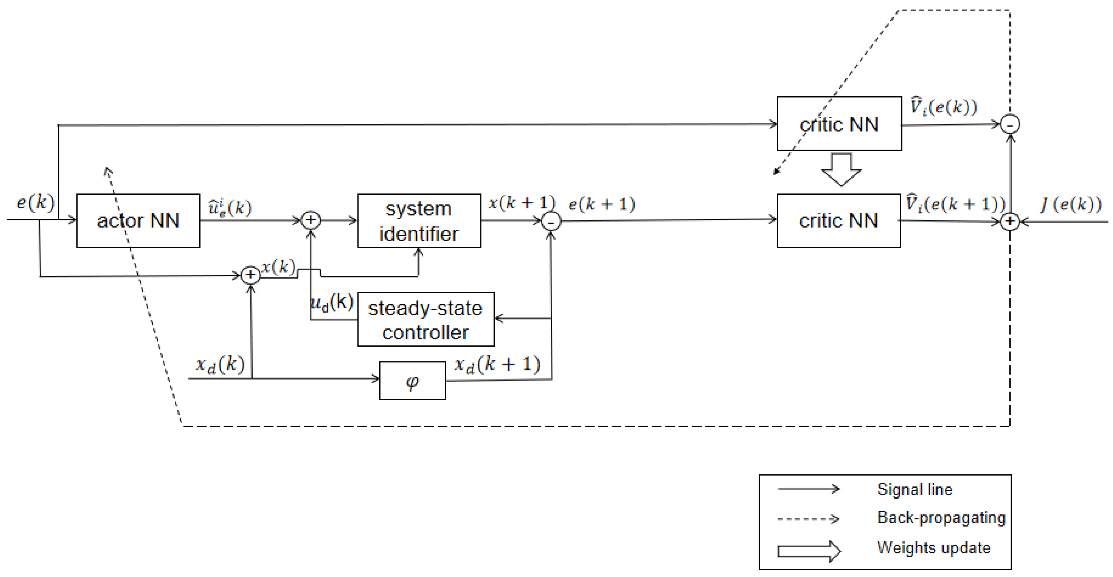
From
Figure 1, it can be seen that with
,
and
, the estimated error
can be obtained with the aid of the RBF-NN identifier and the steady-state controller. Using the steady-state controller, we can obtain the reference trajectory
corresponding to the steady-state controller
. Using the ADP algorithm, we can obtain optimal feedback controller
. Then, the actual controller
and system dynamic
can be obtained. Furthermore, with
and
we can get the estimated tracking error
,further obtained
. Finally, we can reconstruct the system dynamic to track the reference trajectory.
Theorem 1.
For the optimal tracking problem (1)-(3), the RBF-NN identifier (16) is used to approximate , the steady-state controller is approximated by the RBF-NN (23), and the feedforward networks (34),(38) is used to approximate the cost function and the feedback controller , respectively. Assume that the parameters satisfy the following inequality,
where η is the learning rate of the RBF-NN identifier, σ and γ are the update parameters of the steady-state controller approximating network weights, is the learning rate of the actor network, is the learning rate of the critic network, and are hidden layer function of the actor network and the critic network. Then, the closed loop system (6) of approximating error is asymptotically stable when the parameter estimation errors are bounded.
Proof. Considering the following positive definite Lyapunov function candidate
where
,
,
,
.
Firstly, differencing it according to the Lyapunov function of
yields
According to the Assumption 2, Assumption 4 and (
42), (
51) can be done to get
After that, differencing it according to the Lyapunov function of
yields
where
Substituting (
54) into (
53) yields
Considering (
26) and
, we can deduce
With Lemma 2 and Lemma 3, we can further deduce
where
is a positive constant.
Next, we consider the following Lyapunov function
Then, differencing it according to the Lyapunov function of (
58) yields
Finally,
is derived from (
52), (
57) and (
59)
Based on the above analysis, when the parameters are selected to fulfill the following condition with
,
we can obtain
. This proof is completed. □
4. Simulation
In this section, in order to demonstrate the effectiveness of the proposed tracking control method, a discrete-time nonlinear system is introduced.The case is derived from [
47]. We assume that the nonlinear smooth function
is an unknown nonlinear drift function and
is a known function. The corresponding
and
are given as
The reference trajectory
for the above system is defined as
where
of y-axis is chosen as k(1,...,10000) multiplied by
in the simulation.
The RBF networks have a three-layer structure with 2 input neurons, hidden layers have 9 neurons, and output layer have 2 neurons, the parameters
and
of the radial basis functions are chosen as
(i=1,2,...,9) =
and
, the initial weights
were chosen to be random numbers between (0,1), where the inputs to the RBF-NN identifier are chosen to be
and the inputs to the RBF-NN steady-state control
are chosen to be
. Update of weights
,
is used in (
21) and (
28). Because
, we can select
. According to
of Theorem 1, we can select
. For the control parameters
, because hidden layers have 9 neurons,
,
, we select
. While control parameters
, we can know
and
from Theorem 1, so selecting
. The initial state is set as
. We trained the RBF networks with 10,000 steps of acquired data , and
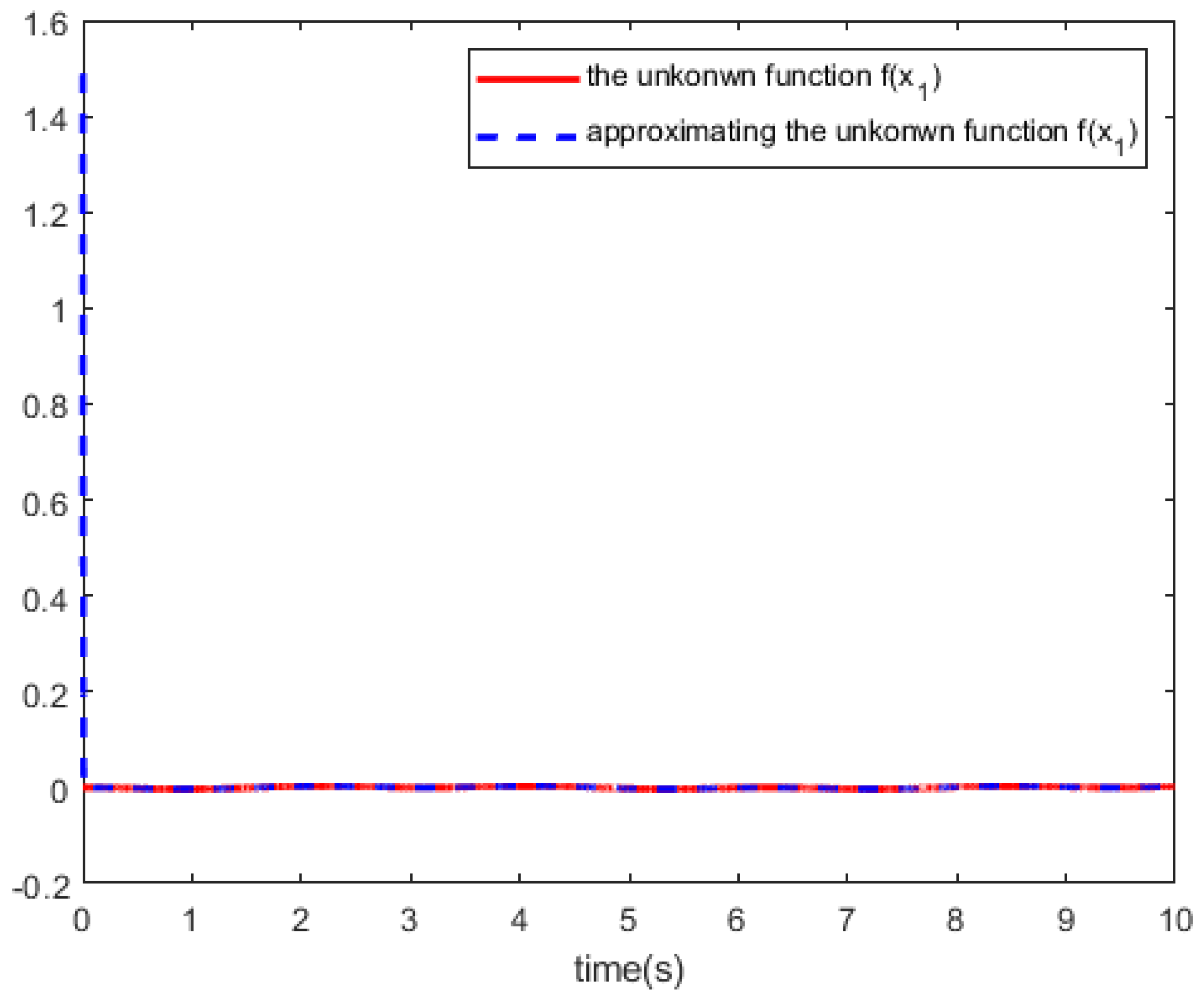
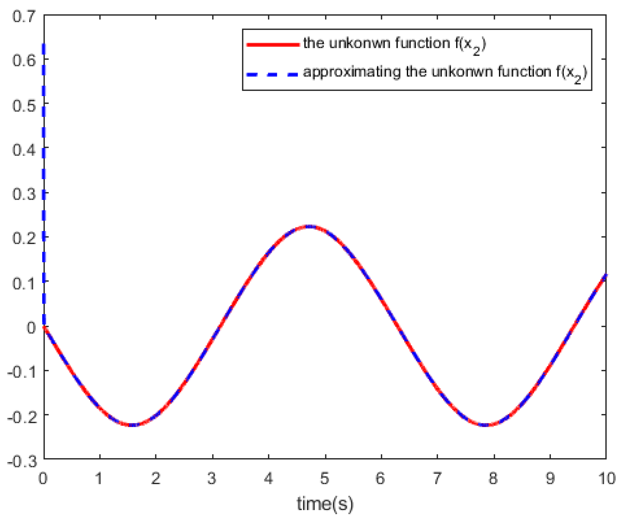
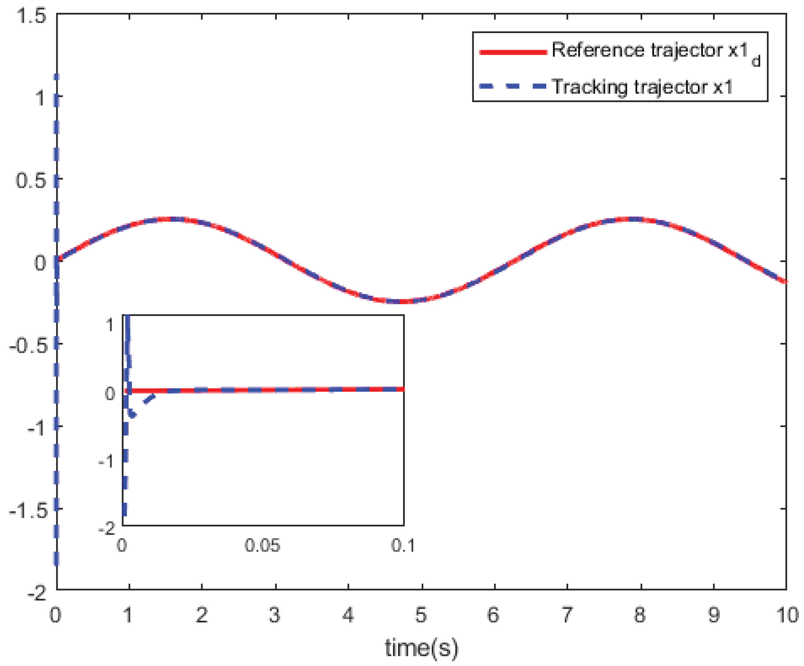
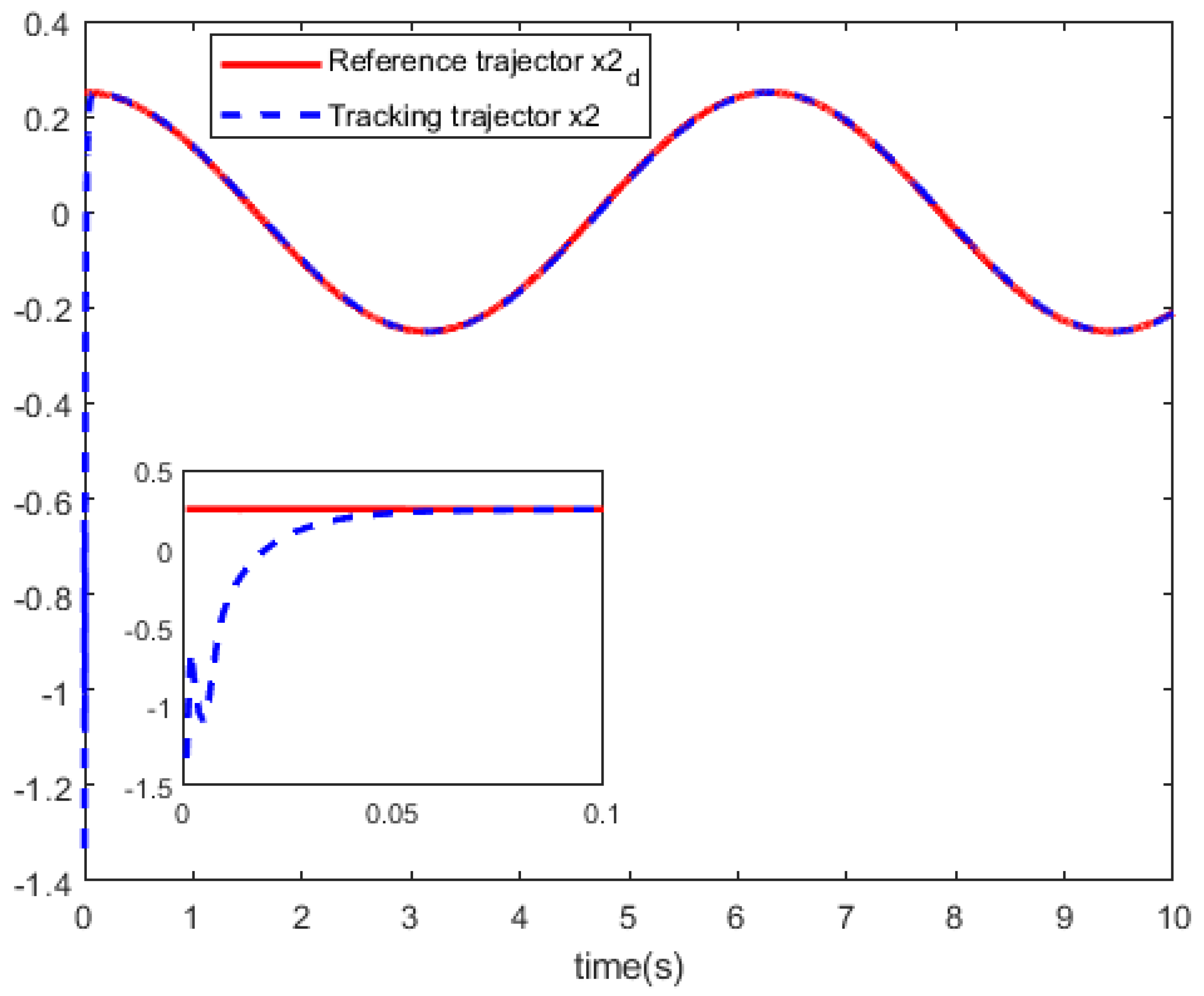
Figure 2 and
Figure 3 shows the RBF-NN identifier to approximate the tracking curves of the unknown dynamics
.
The performance index is select as
and
that
I is the identity matrix with appropriate dimension. For the actor network and critic network, we used the same parameter settings. The initial weights of the critic network and the actor network are chosen as random numbers between
. The input layer have 2 neurons, the hidden layer have 15 neurons, the output layer have 2 neurons, the learning rate is 0.1. The hidden layer uses the function
and the function
, the output layer uses the function
.Though parameter settings, we train the actor network and the critic network with 5000 training steps to reach the given accuracy 1e-9.
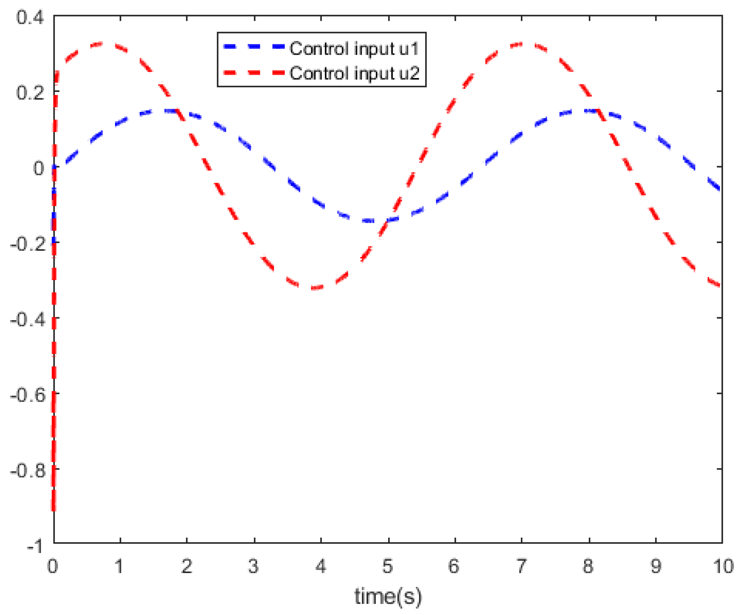
Figure 4 shows the curves of the system control
u. In
Figure 5 and
Figure 6, we can see the curves of the state trajector
x and the reference trajector
.
Based on above the results, the simulation results show that this tracking technique obtains a relatively satisfactory tracking performance for partially unknown discrete-time nonlinear systems.
5. Conclusion
This paper proposed an optimal tracking control scheme through approximate dynamic programming for a class of partially unknown discrete-time nonlinear systems based on RBF-NNs . In dealing with unknown variables, two RBF-NNs are used to approximate the unknown function and the steady-state controller, respectively. Moreover, ADP algorithm are introduced to get the optimal feedback control for tracking the error dynamics, two feedforward neural networks are utilized as structures to approximate the cost function and feedback control inputs severally. Finally, simulation results show a relatively satisfactory tracking performance, which verify the effectiveness of the optimal tracking control technique. In future works, we will consider event-triggered control as well as completely unknown dynamics.
Author Contributions
All the authors contributed equally to the development of the research. All authors have read and agreed to the published version of the manuscript.
Funding
This research was funded by the National Natural Science Foundation of China under Grant No. 61463002, the Guizhou Province Natural Science Foundation of China under Grant No. Qiankehe Fundamentals-ZK[2021] General 322 and the Doctoral Foundation of Guangxi University of Science and Technology Grant No. Xiaokebo 22z04.
Informed Consent Statement
Not applicable.
Data Availability Statement
Data is contained within the article.
Acknowledgments
The authors thank to the Journal editors and the reviewers for their helpful suggestions and comments.
Conflicts of Interest
The authors declare no conflict of interest.
References
- Broomhead, D.S.; Lowe, D. Radial basis functions, multi-variable functional interpolation and adaptive networks. 1988. [Google Scholar]
- Narendra, K.S.; Parthasarathy, K. Identification and control of dynamical systems using neural networks. IEEE Transactions on Neural Networks 1990, 1. [Google Scholar] [CrossRef] [PubMed]
- Narendra, K.S.; Mukhopadhyay, S. Adaptive control of nonlinear multivariable systems using neural networks. 1994; 737–752. [Google Scholar]
- Hartman, E.J.; Keeler, J.D.; Kowalski, J.M. Layered Neural Networks with Gaussian Hidden Units as Universal Approximations. Neural Computation 1990, 210–215. [Google Scholar] [CrossRef]
- Park, J. Universal approximation using radial basis function networks. Neural Comput. 1993. [Google Scholar] [CrossRef]
- Lewis, F.L.; Yesildirek, A.; Liu, K. Multilayer neural-net robot controller with guaranteed tracking performance. IEEE Transactions on Neural Networks 1996, 7. [Google Scholar] [CrossRef] [PubMed]
- Kobayashi, H.; Ozawa, R. Kobayashi, Hiroaki , and R. Ozawa . Adaptive neural network control of tendon-driven mechanisms with elastic tendons. Automatica 2003, 1509–1519. [Google Scholar] [CrossRef]
- Lewis, F.L.; et al. Optimal Control, 3rd ed.; John Wiley & Sons, Inc.: New Jersey, 2012. [Google Scholar]
- Mannava, A.; et al. Optimal tracking control of motion systems. IEEE Trans. Control Syst. Technol. 2012, 1548–1558. [Google Scholar] [CrossRef]
- Sharma, R.; Tewari, A. Optimal nonlinear tracking of spacecraft attitude maneuvers. IEEE Trans. Control Syst. Technol. 2013, 12, 677–682. [Google Scholar] [CrossRef]
- Bellman, R.E. Dynamic Programming. Princeton University Press: Princeton, NJ, 1957. [Google Scholar]
- Lewis, F.L.; Syrmos, V.L. Optimal Control; Wiley: New York, 1995. [Google Scholar]
- Powell, W.B. Approximate Dynamic Programming: Solving the Curses of Dimensionality; Wiley: New York, NY, USA, 2009. [Google Scholar]
- Bertsekas, D.P.; Tsitsiklis, J.N. Neuro-Dynamic Programming; Athena Scientifific: Belmont, MA, USA, 1996. [Google Scholar]
- Si, J.; Barto, A.G.; Powell, W.B.; Wunsch, D. Handbook of Learning and Approximate Dynamic Programming; Wiley: New York, NY, USA, 2004. [Google Scholar]
- Sutton, R.S.; Barto, A.G. Reinforcement Learning: An Introduction; MIT Press: Cambridge, MA, USA, 1998. [Google Scholar]
- Lewis, F.L.; Vrabie, D. Reinforcement learning and adaptive dynamic programming for feedback control. IEEE Circuits Syst. 2009, 8, 32–50. [Google Scholar] [CrossRef]
- Lewis, F.L.; Vrabie, D.; Vamvoudakis, K.G. Reinforcement learning and feedback control: Using natural decision methods to design optimal adaptive controllers. IEEE Control Syst. 2012, 11, 76–105. [Google Scholar] [CrossRef]
- Lewis, F.L.; Liu, D. Reinforcement Learning and Approximate Dynamic Programming for Feedback Control; Wiley: Hoboken, NJ, USA, 2013. [Google Scholar]
- Fairbank, M.; Li, S.; Fu, X.; Alonso, E.; Wunsch, D. An adaptive recurrent neural-network controller using a stabilization matrix and predictive inputs to solve a tracking problem under disturbances. Neural Netw. 2014, 1, 74–86. [Google Scholar] [CrossRef]
- Vrabie, D.; Lewis, F. Neural network approach to continuous-time direct adaptive optimal control for partially unknown nonlinear systems. Neural Netw. 2009, 4, 237–246. [Google Scholar] [CrossRef]
- Liu, D.; Yang, X.; Li, H. Adaptive optimal control for a class of continuous-time affifine nonlinear systems with unknown internal dynamics. Neural Comput. Appl. 2013, 11, 1843–1850. [Google Scholar] [CrossRef]
- Bhasin, S.; Kamalapurkar, R.; Johnson, M.; Vamvoudakis, K.G.; Lewis, F.L.; Dixon, W. E. A novel actor–critic–identififier architecture for approximate optimal control of uncertain nonlinear systems. Automatica 2013, 1, 82–92. [Google Scholar] [CrossRef]
- Al-Tamimi, A.; Lewis, F.L.; Abu-Khalaf, M. Discrete-time nonlinear HJB solution using approximate dynamic programming: Convergence proof. IEEE Trans. Syst. Man Cybern. B Cybern. 2008, 8, 943–949. [Google Scholar] [CrossRef]
- Prokhorov, D.V.; Wunsch, D.C. Adaptive critic designs. IEEE Trans. Neural Netw. 1997, 9, 997–1007. [Google Scholar] [CrossRef] [PubMed]
- Luo, Y.; Zhang, H. Approximate optimal control for a class of nonlinear discrete-time systems with saturating actuators. Prog. Natural Sci. 2008, 1023–1029. [Google Scholar] [CrossRef]
- Dierks, T.; Jagannathan, S. Online optimal control of nonlinear discrete-time systems using approximate dynamic programming. Control Theory Appl. 2011, 361–369. [Google Scholar] [CrossRef]
- Si, J.; Wang, Y.-T. Online learning control by association and reinforcement. IEEE Trans. Neural Netw. 2001, 5, 264–276. [Google Scholar] [CrossRef] [PubMed]
- Ren, L.; Zhang, G.; Mu, C. Data-based H∞ control for the constrained-input nonlinear systems and its applications in chaotic circuit systems. IEEE Trans. Circuits Syst. 2020, 8, 2791–2802. [Google Scholar] [CrossRef]
- Zhao, F.; Gao, W.; Liu, T.; Jiang, Z.P. Event-triggered robust adaptive dynamic programming with output-feedback for large-scale systems. IEEE Trans. Control Netw. Syst. 2023, 8, 63–74. [Google Scholar] [CrossRef]
- Wei, Q.; Li, H.; Yang, X.; He, H. Continuous-time distributed policy iteration for multicontroller nonlinear systems. IEEE Trans. Cybern. 2021, 5, 2372–2383. [Google Scholar] [CrossRef] [PubMed]
- Zhang, Y.; Zhao, B.; Liu, D.; Zhang, S. Event-triggered control of discrete-time zero-sum games via deterministic policy gradient adaptive dynamic programming. IEEE Trans. Syst., Man, Cybern., Syst. 2022, 8, 4823–4835. [Google Scholar] [CrossRef]
- Zhu, Y.; Zhao, D.; He, H. Invariant adaptive dynamic programming for discrete-time optimal control. IEEE Trans. Syst., Man, Cybern., Syst. 2020, 11, 3959–3971. [Google Scholar] [CrossRef]
- Wei, Q.; Han, L.; Zhang, T. piking adaptive dynamic programming based on poisson process for discrete-time nonlinear systems. IEEE Trans. Neural Netw. Learn. Syst. 2022, 5, 1846–1856. [Google Scholar] [CrossRef]
- Yang, Y.; Wunsch, D.; Yin, Y. Hamiltonian-driven adaptive dynamic programming for continuous nonlinear dynamical systems. IEEE Trans. Neural Netw. Learn. Syst. 2017, 8, 1929–1940. [Google Scholar] [CrossRef]
- Li, M.; Qin, J.; Freris, N.M.; Ho, D.W. Multiplayer Stackelberg– Nash game for nonlinear system via value iteration-based integral reinforcement learning. IEEE Trans. Neural Netw. Learn. Syst. 2022, 4, 1429–1440. [Google Scholar] [CrossRef] [PubMed]
- Guo, X.; Yan, W.; Cui, R. Integral reinforcement learning-based adaptive NN control for continuous-time nonlinear MIMO systems with unknown control directions. IEEE Trans. Syst., Man, Cybern., Syst. 2020, 11, 4068–4077. [Google Scholar] [CrossRef]
- Xue, W.; Fan, J.; Lopez, V.G.; Jiang, Y.; Chai, T.; Lewis, F.L. Off-policy reinforcement learning for tracking in continuous-time systems on two time scales. IEEE Trans. Neural Netw. Learn. Syst. 2021, 10, 4334–4346. [Google Scholar] [CrossRef]
- Sun, C.; Li, X.; Sun, Y. A parallel framework of adaptive dynamic programming algorithm with off-policy learning. IEEE Trans. Neural Netw. Learn. Syst. 2021, 8, 3578–3587. [Google Scholar] [CrossRef]
- Duan, J.; Guan, Y.; Li, S.E.; Ren, Y.; Sun, Q.; Cheng, B. Distributional soft actor-critic: Off-policy reinforcement learning for addressing value estimation errors. IEEE Trans. Neural Netw. Learn. Syst. 2022, 11, 6584–6598. [Google Scholar] [CrossRef]
- Qiao, L.; et al. A novel optimal tracking control scheme for a class of discrete-time nonlinear systems using generalised policy iteration adaptive dynamic programming algorithm. Syst. Sci. 2017, 525–534. [Google Scholar] [CrossRef]
- Kiumarsi, B.; Lewis, F.L. Actor-critic-based optimal tracking for partially unknown nonlinear discrete-time systems. IEEE Trans. Neural Networks Learn. Syst. 2017, 140–151. [Google Scholar] [CrossRef] [PubMed]
- Zhang, H.; et al. Optimal tracking control for a class of nonlinear discrete-time systems with time delays based on heuristic dynamic programming. IEEE Trans. Neural Networks 2011, 1851–1862. [Google Scholar] [CrossRef] [PubMed]
- Zhang, H.; Wei, Q.; Luo, Y. A Novel Infinite-Time Optimal Tracking Control Scheme for a Class of Discrete-Time Nonlinear Systems via the Greedy HDP Iteration Algorithm. IEEE Trans. Syst., Man, Cybern., Syst. 2008, 937–942. [Google Scholar] [CrossRef] [PubMed]
- Song, S.; Zhu, M.; Dai, X.; Gong, D. Model-Free Optimal Tracking Control of Nonlinear Input-Affine Discrete-Time Systems via an Iterative Deterministic Q-Learning Algorithm. IEEE Trans. Neural Networks Learn. Syst. 2024, 1, 999–1012. [Google Scholar] [CrossRef]
- Huang, Y.; Liu, D. Neural-network-based optimal tracking control scheme for a class of unknown discrete-time nonlinear systems using iterative ADP algorithm. Neurocomputing 2014, 46–56. [Google Scholar] [CrossRef]
- Dierks, T.; Jagannathan, S. Optimal tracking control of affine nonlinear discrete-time systems with unknown internal dynamics. In Proceedings of the IEEE Conference on Decision & Control IEEE; 2010. [Google Scholar] [CrossRef]
- Zhang, J.; Ge, S.S.; Lee, T.H. Direct RBF neural network control of a class of discrete-time non-affine nonlinear systems. In Proceedings of the American Control Conference; 2002. [Google Scholar]
- Ge, S.S.; Zhang, J.; Lee, T.H. Adaptive MNN control for a class of non-affine NARMAX systems with disturbances. Systems & Control Letters 2004, 53, 1–12. [Google Scholar] [CrossRef]
|
Disclaimer/Publisher’s Note: The statements, opinions and data contained in all publications are solely those of the individual author(s) and contributor(s) and not of MDPI and/or the editor(s). MDPI and/or the editor(s) disclaim responsibility for any injury to people or property resulting from any ideas, methods, instructions or products referred to in the content. |
© 2024 by the authors. Licensee MDPI, Basel, Switzerland. This article is an open access article distributed under the terms and conditions of the Creative Commons Attribution (CC BY) license (http://creativecommons.org/licenses/by/4.0/).
