Preprint
Article

Synergizing Transfer Learning and Multi-Agent Systems for Thermal Parametrization in Induction Traction Motors

Altmetrics

Downloads

82

Views

39

Comments

0

A peer-reviewed article of this preprint also exists.

This version is not peer-reviewed

Submitted:

01 March 2024

Posted:

01 March 2024

You are already at the latest version

Alerts
Abstract
This paper presents an innovative multi-agent, data-driven reinforcement learning (RL) approach to develop and utilize the thermal equivalent network model that represents the motor's thermal dynamics. A multi-agent reinforcement learning is designed and trained to adjust the model parameters using data from several motor driving cycles. To ensure the incoming driving cycle matches the historical data before employing the pre-trained RL agents, offline statistical analysis and clustering techniques are developed and used. Numerical simulations highlighted the RL agent's ability to develop strategies that effectively address the variability of driving cycles. The proposed RL framework showed its capability to accurately reflect the motor's thermal behavior under various driving conditions.
Keywords: 
Subject: Engineering  -   Control and Systems Engineering

1. Introduction

Induction motors are widely preferred in railway applications due to their mechanical robustness, high overload capacity and affordability [1]. However, maintaining the optimum temperature in traction motors is crucial for maximizing their efficiency and keeping safe and reliable operation in railway propulsion systems. The traction motors operate in fluctuating load demand and ambient conditions potentially causing overheating of some parts such as windings resulting in motor failures. Hence, temperature monitoring in real time is deemed to be necessary. Conventionally, an accurate estimation of the temperatures is performed using detailed physics-based thermal models. However, the computational demand of such techniques limits their adaptability to real-world conditions. Hence, prior calibration of the thermal models in a controlled experimental environment is performed. The introduction of digital technologies such as smart sensors, and the Internet of Things (IoT), has transformed the way thermal model parameters are calibrated, in the current scenario. These technologies enable a shift from conventional, lab-based calibration methods to real-time analysis of operational data. Utilizing IoT and smart sensors for constant monitoring leads to early identification of thermal issues. Which results in decreasing the chance of system failures and improves predictive maintenance and operational efficiency.
In recent years, the surge of interest in machine learning (ML) techniques has been considered promising tools for automating monitoring and control in induction motor drivers. These data-driven models [2], particularly employing neural networks, offer promising results in temperature prediction and parameter estimation. A machine learning model can be trained to empirically estimate temperature using data collected from test benches [2]. Moreover, supervised ML models have been explored for real-time estimation of parameters such as rotor resistance in in-duction motor control systems. Recurrent neural networks (RNNs) and convolutional neural networks (CNNs) are widely used for sequence learning tasks and can manage high-dynamic nature scenarios. Additionally, reinforcement learning (RL) has emerged as another promising data-driven approach for electric motor drive control [3]. RL techniques, which learn through trial and error without the need for supervised data labeling, rely on a reward function to guide the learning process. This allows for continuous improvement of control policies based on feedback, showcasing the evolving landscape of ML applications in motor drive monitoring and control.
This work contributes to the scientific endeavor of employing a data-driven reinforcement learning-based model for parameter estimation and precise prediction from thermal models using measured and tool driving cycles data. The selection of a reinforcement learning agent is critically influenced by the driving cycle data pattern and the specific problem it aims to solve. This approach not only challenges traditional calibration methods but also contributes to the development of more adaptive and efficient thermal management strategies for railway propulsion systems.
The structure of this paper is outlined as follows: A background and related work is presented in Section 2. Section 3 introduces the multiple agents reinforcement learning (RL) framework developed for the optimization of the model. Details regarding the dataset and the training methodology are also discussed in Section 3. Section 4 presents and analyzes the outcomes of the thermal model. Finally, Section 5 offers concluding thoughts and directions for future research.

2. Background and Related Work

Traction drive systems are subjected to dynamically changing operating conditions, thus, making tracking of the temperature during run time imperative to prevent any thermal overloading. Optimizing the motor utilization in terms of generating maximum torque and power can lead to a high current load, hence more heat load in the windings. This thermal overloading phenomenon increases the possibility of motor failure if the temperature exceeds the rated temperature withstanding capacity in the insulation. In-duction motor drives are the most used motors in railway propulsion applications to date because of their high efficiency, reliability, mechanical robustness, and low cost [4]. These motors’ performance varies nonlinearly with temperature, frequency, saturation, and operating point which makes temperature monitoring essential to feedback the controller to compensate for the electrical signals such as voltage and current.
There are several established direct or indirect means for estimating the temperature in different motor parts. Direct methods such as installing contact-based sensors in stator and rotor parts are the simplest means for measurement. For the rotating parts, the data transmission needs special arrangement; to be conducted with the help of end slip rings, or telemetry means. Regardless, installing sensors requires integration effort and additional cost and adds complexity due to their inaccessibility for replacement in case of failures or detuning. Hence model-based measurement techniques have been focused on the past decade [5,6]. Here the temperatures can be estimated from the measurement of temperature-dependent electrical parameters in both offline and online manner. In these approaches, the model dynamic behaviors must be accurately accounted for to avoid any estimation errors. These are also invasive in nature and create disturbance to normal operation [7].
Thermal analysis using computational fluid dynamics or heat equation-based finite element analysis method potentially exhibits good accuracy in temperature estimation. However, both these approaches demand rigorous modeling effort and hence require high computational resources. Thus, it has been excluded from real-time monitoring upfront. An alternative but accurate computationally light temperature estimation technique is using the lumped-parameter thermal network (LPTN) model. An LPTN model summarizes the heat transfer process and can be represented in thermal equivalent circuit diagrams based on heat transfer theory. In the LPTN model, the heat conduction and convection phenomena are represented as thermal resistances and capacitance between different nodes. Furthermore, electro-mechanical power conversion losses, such as winding losses, core losses and mechanical and windage losses are provided as inputs to the LPTN model to compute the temperature.
The complexity of LPTN models depends on the number of chosen nodes in the network. Generally, white box LPTN, based on pure analytical equations, are more accurate but are endowed with many thermal parameters, which could be complex to calculate in practice [8]. A reduced-order structure with fewer nodes is computationally lightweight and, hence, more suitable for online deployment. In this approach only the dominant heat transfer pathways are represented hence expert domain knowledge is essential not only for the choice of structural design but also for their parameter values. In the past, several reduced order models, typically categorized as light grey (with 5-15 nodes) or dark grey (with 2-5 nodes) LPTN models were structured to estimate the temperatures. The use of reduced-order LPTN models would require estimations of many parameters that are not well known or possible to calculate using analytical equations [9,10]. Thus, the identification of the parameters through empirical-based tuning is a crucial step in these studies [11,12,13]. The parameter identification procedure can be stated as an optimization problem, in which the values are varied until the used LPTN model gives the same results as the experimental ones. Several gradient and non-gradient-based optimization methods are used for identifying the parameters. In the work presented by [11], the parameter identification is conducted by using determinist inverse-based methods such as the Gauss-Newton method, the Levenberg-Marquardt method, and stochastic inverse-based methods such as the Genetic Algorithms.
The thermal parameter values for a traction motor are non-constant due to nonlinear thermal effects. The convective heat transfer coefficients within the air gap as well as in the end-cap region are nonlinearly dependent on the rotor speed and the ambient temperature. In a similar line, in an air-cooled motor, the heat transfer from the stator frame is dependent on the ambient temperature and airflow rate. Sciascera et al. [9] employed a parameter tuning procedure based on a sequential quadratic programming iterative method for obtaining the uncertain thermal parameters in the LPTN. However, the computational cost of such tuning procedures is high due to the time-variant nature of the parameters. Furthermore, to improve computational efficiency, the dependence of the state matrix on the phase current is approximated with polynomial approximation.
The loss components such as the winding losses which are input to the LPTN model can be calculated for the measured current and winding resistance. The resistance values are temperature dependent which is a state variable in the thermal matrix. Furthermore, the core loss is not measurable. A usual approach to determining iron losses is measuring total power losses and subtracting winding losses. Hence, all errors in the determination of total and winding losses directly add up to an error in the iron loss values. To deal with these uncertainties, Gedlu et al. [14] used an extended iron loss model as input to a low-order LPTN model for temperature estimation. The loss inputs as a form of spatial loss model calculate individual core losses for each node. In addition to the heat transfer coefficients, the uncertain parameters in the core loss equations are tuned in their possible searching space using particle swarm optimization (PSO) to minimize the estimation error in comparison to empirical measurements.
Xiao and Griffo [13] in their work presented an online measurement-informed thermal parameter estimation using a recursive Kalman filter method. While a pulse width modulation-based estimation method is utilized for rotor temperature measurement, the temperatures in three nodes such as stator core, winding, and rotor are predicted. The input losses for the LPTN model are derived based on a model-based approach and with the use of Finite Elements analysis. The identification problem is formulated as a state observer with eight states. Three of the states correspond to the nodes’ temperatures and the rest five states represent the unknown thermal resistance parameters in the LPT network. The nonlinearity of the model is dealt with continuously updated linearization of the extended Kalman filter method.
As described by Wallscheid [7], parameter identification can be made in a local approach or a global approach. In the work presented by [12], a three-node LPTN is parametrized based on a global approach. A sequence of interdependent identification steps was followed, and the experimental data were used to find the thermal parameters. The model uses the measurement-based loss inputs available with motor Electrical Control Unit quantities, such as motor speed and electric currents. The parameter identification approach has been built on the idea of mapping the linear time-varying parameters to a set of time-invariant models operating within a certain chosen environment. Thus, a consistent parameter set for the whole operating region could be obtained with the adaptation of the relevant boundary conditions through various identification cycles. Wallscheid [27] used PSO combined with a sequential quadratic programming technique to identify the varying thermal parameters of a four-node LPTN model. The power loss measurement was made in the complete operation range while keeping the temperature constant at the nodes. The loss distribution among the nodes is interpreted as part of the parameter identification procedure to deal with the uncertainty.
While the global approach is more robust in capturing all operating regions of the machine than the local approach, it can also be problematic if the parameter landscape to be identified is large and highly nonlinear in nature [7].
The growing interest and upsurge in machine learning (ML) techniques in the past decade make these potentially viable tools in the area of automated monitoring and motor drive control. A pure machine ML model is excluded from the expert knowledge of any classic fundamental heat theory and does the task of estimating the temperature empirically. Under this platform, the model parameters are fitted based on collected testbench/observation data only [2,15]. The widely used ML algorithm is the linear regression technique which has a low computational complexity and is used for temperature predictions [16,17]. However, as linear regression is a linear time-invariant, it does not capture the dynamics of a machine model.
In the field of sequential learning tasks in highly dynamic environments, recurrent neural networks and convolutional neural networks are the state of the art in classification and estimation performance. In the study conducted by Kirchgässner et al. [16], deep recurrent and convolutional neural networks with residual connections are empirically evaluated for predicting temperature profile in the stator teeth, winding, and yoke as well. The concept is to parameterize neural networks entirely on empirical data, without being driven by the domain expertise. Furthermore, supervised ML models are also investigated for online parameter estimation such as rotor resistance and mutual inductance in the control system of an induction motor [18]. In the presented work, a simple two-layer artificial neural network (ANN) is trained by minimizing the error between the rotor flux linkages based on an IM analytical voltage model and the output of the ANN-trained model. Feedforward and recurrent networks are used to develop an ANN as a memory for remembering the estimated parameters and for computing the electrical parameters during the transient state.
While data-driven methods are effective in predicting the temperature, the tuned parameters are not interpretable and could not be designed with the low amount of model parameters as in an LPTN model at equal estimation accuracy. As a further development, to make expert knowledge-based calibration less desirable and to account for the uncertainties regarding the input power losses, Kirchgässner [19] proposed a deep learning-based temperature model where a thermal neural network is introduced, which unifies both consolidated knowledge in the form of heat-transfer-based LPTNs, and da-ta-driven nonlinear function approximation with supervised machine learning.
The reinforcement learning (RL) based method is another promising data-driven technique explored in the field of control of electric machine drives [20,21]. RL methods enable learning in a trial-and-error manner and avoid supervision of each data sample. The algorithm requires a reward function to receive the reward signals throughout the learning process. Thus, the control policy could be improved continuously based on the measurement feedback. In this paper, a data-driven reinforcement learning-based parametrization method is proposed to tune a thermal model in induction traction motors. In the following section, the parameterized model is developed, and the reinforcement learning framework is presented.
3. Multiple Agents Reinforcement Learning Based Framework

3.1. The Reinforcement Learning Framework

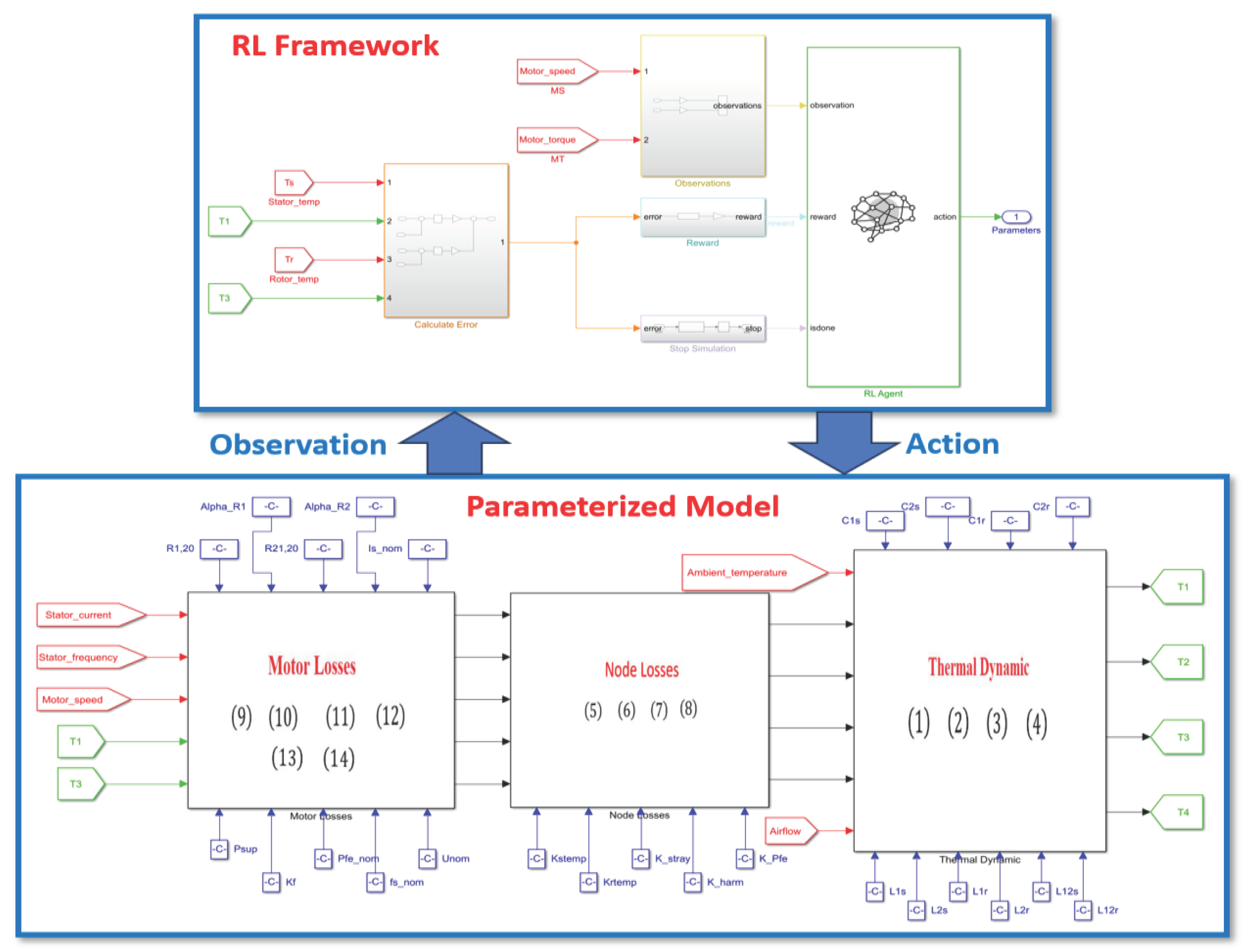
A data-driven reinforcement learning-based parametrization method was proposed in our previous work [22] to calibrate a thermal model of an induction traction motor as depicted in Figure 1. This model encapsulates the dynamic behavior of an induction motor's temperature (see Appendix A for the thermal model description). Stator current and frequency, motor velocity, cooling airflow, rotor temperature, torque and ambient temperature were given as input to the thermal model. The parameterized model rigorously evaluates the reinforcement learning policies for the identification of optimized parameters. The RL framework includes an RL agent, a reward function, observations and actions taken by the agent. Observations represent the data that the RL agent collects from the parametrized model which includes direct measurements such as motor speed (MS) and torque (MT). These measurements help the RL agents to detect changes in the operational conditions. There are indirect measurements such as stator and rotor temperatures and model outputs which are utilized for reward calculation. The reward function produces a value that indicates how effective an agent's action is and guides it toward achieving its goal. This function is crucial in reducing the difference between actual and predicted temperatures.

3.2. RL Multiple Agents Composition

Precise temperature prediction based on controller driving cycles is essential for improving efficiency and safety. The RL agent integrates the policy and a learning strategy in order to map the observations to actions. The system uses both critic and actor networks in which the critic network predicts future rewards based on current actions and observations. Whereas the actor selects the actions to maximize these rewards The proposed data-driven approach employs three distinct reinforcement learning agents, Twin Delayed Deep Deterministic Policy Gradient (TD3), Soft Actor-Critic (SAC), and Deep Deterministic Policy Gradient (DDPG). These agents are used to predict temperature based on nine driving cycles from the tool and one driving cycle based on real measurements. The selection of multiple RL agents depends on certain criteria like data variation and temporal aspects of each driving cycle data. For instance, the SAC agent uses an entropy-based exploration method for driving cycles with unpredictable temperature fluctuations. Conversely, TD3 and DDPG agents use deterministic policy gradients for more stable and predictable cycles. A TD3 algorithm is recognized for its efficacy in continuous environments that facilitate policy improvement and episodic training. In the proposed approach, the architecture of the neural network, particularly the number of neurons, plays a critical role in the precision of stator and rotor temperature predictions.
Our analysis reveals that the configuration of neurons varies significantly across different driving cycles and agents. For instance, having more neurons in the hidden layers of the SAC agents’ neural network has led to better predictions for driving cycles with lots of temperature changes. This is because a complex deep neural network can better understand complex data patterns. However, adding more neurons does not always result in improved results for every agent or driving cycle data. Our findings highlight the need for customizing the selection and deep neural network of the reinforcement learning agent to obtain precise temperature predictions from various controller driving cycle data.

3.3. RL Agent Training Process

3.3.1. Dataset Description

For the reinforcement learning (RL) multiple agent training, the dataset utilized recordings from an induction motor under nine varied driving cycles and one driving cycle from measured data. This dataset includes motor speed, torque, airflow, stator current and frequency, motor voltage, and stator and rotor winding temperature. Whereas measured data includes motor speed, torque, stator current, motor voltage, and stator temperatures. Given the diversity in sampling frequencies and missing values within the data, a preprocessing step involves resampling and interpolating to ensure a uniform and complete dataset. This dataset is employed within a parameterized model that simulates an unfamiliar environment for the agent.

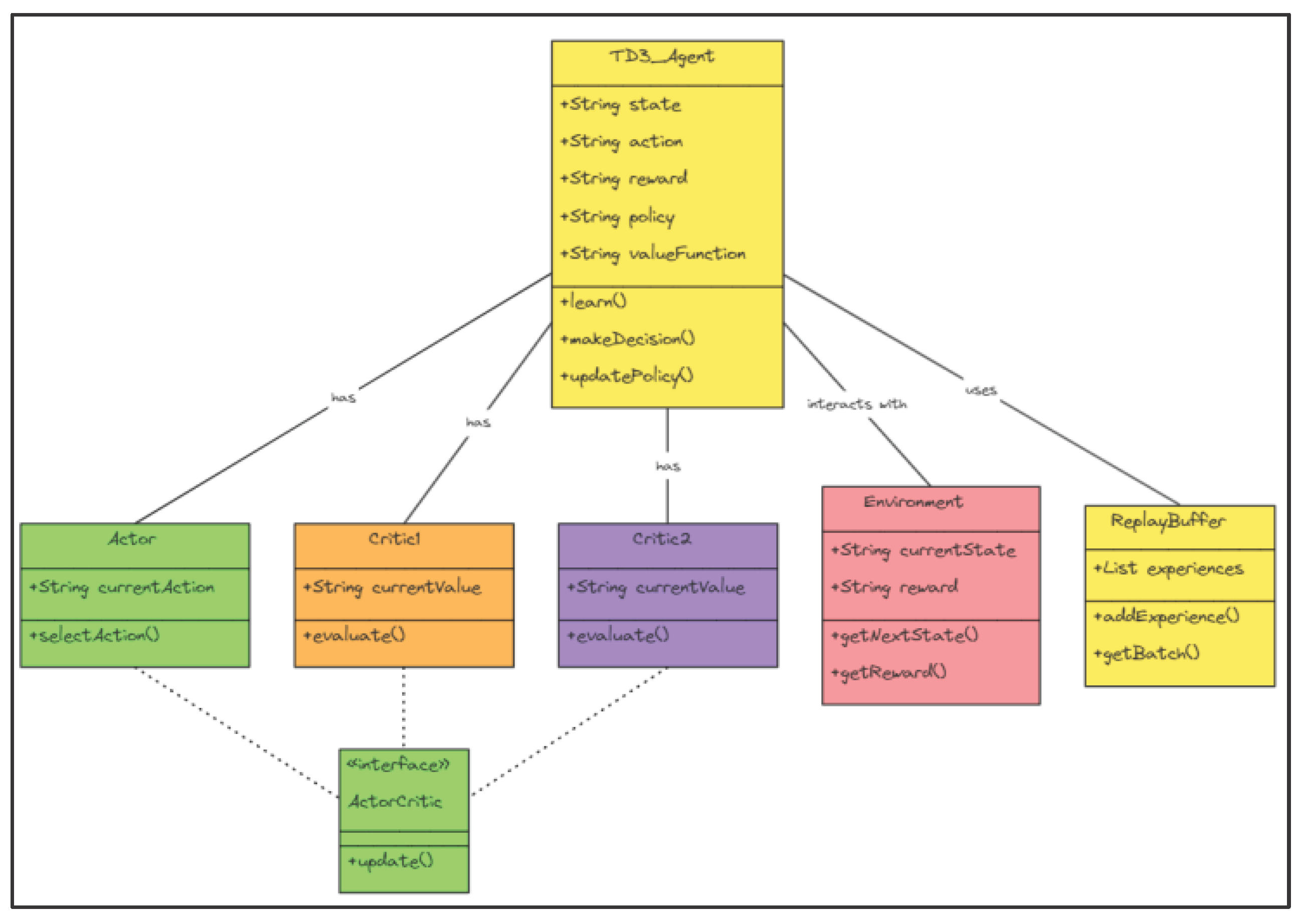
3.3.2. The TD3 Structure

The Twin-Delayed Deep Deterministic Policy Gradient (TD3) strategy employs a single-actor network with two critic networks as shown in Figure 2. These networks are deep neural networks that use observations, actions, and rewards which are gathered from the experience replay buffer. Experience replay buffer stores past experiences to allow the learning algorithm to benefit from a wide range of scenarios. The TD3 algorithm ensures that the actor and critic models are effectively trained to predict and evaluate the output of actions taken in the actual environment.

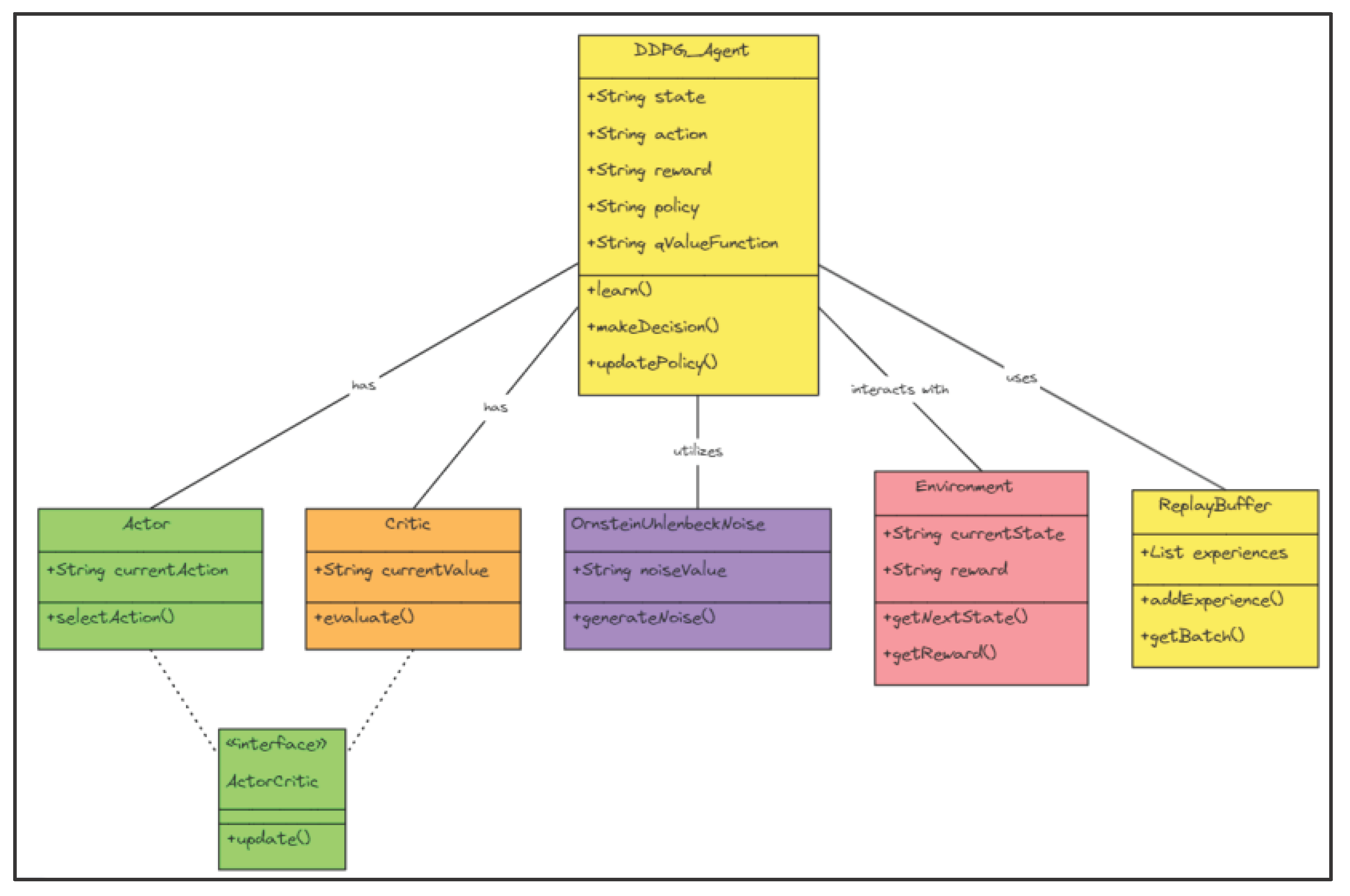
3.3.3. DDPG Agent Structure

The Deep Deterministic Policy Gradient (DDPG) agent combines the benefits of both policy gradient and value-based approaches. This framework excels in managing high-dimensional, continuous action spaces, making it particularly suitable for complex control tasks. The DDPG framework consists of four key components as shown in Figure 3 such as an actor network that proposes actions. A critic network evaluates the actions' potential reward and a target actor and critic network. These components use a replay buffer to store experiences and an update mechanism is used to combine target network parameters with main networks.

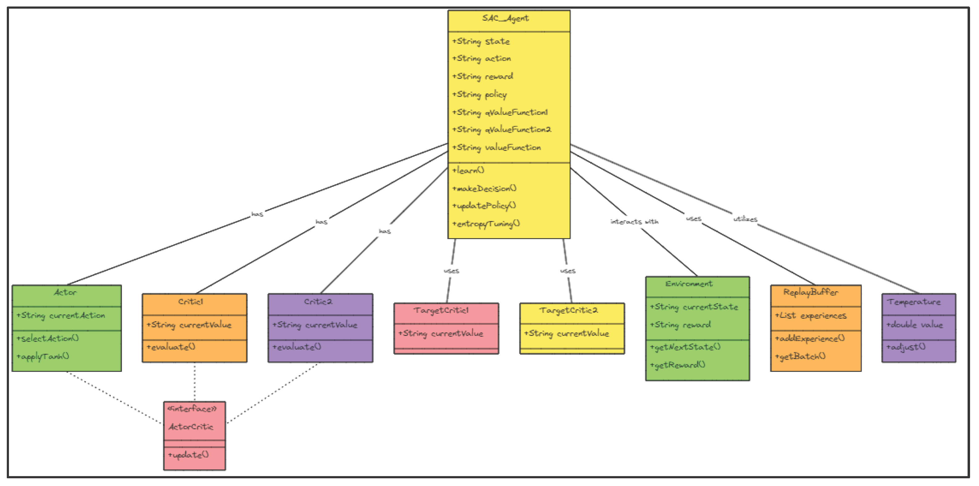
3.3.4. SAC Agent Structure

The Soft Actor-Critic (SAC) agent represents an advanced reinforcement learning strategy that emphasizes entropy in the policy for exploration. The SAC agent comprises of dual critic design to minimize overestimation bias, as shown in Figure 4. The minimum value between two critics is considered to update the value network and actor. The use of entropy in the objective function boosts the agent to discover and exploit the optimal policy in complex environments.

3.4. The Training Process

The training of reinforcement learning (RL) agents as shown in Figure 5 is structured using an episodic approach, with each task considered as an episode. An episode includes the entire cycle of interactions between the agent and its environment. This episodic methodology allows the RL agent to systematically improve its decision-making capabilities by learning from diverse scenarios. Within this framework, the actor network determines an action based on the current observation and its anticipated Q-value. This selected action, observation and the reward received are stored in the experience replay buffer. This buffer is then used to adjust the critic network parameters by reducing a loss function.

3.5. Pretrained Models or Offline Prediction

In addition to online training, our RL framework stores data from interactions within a simulated thermal model environment. After undergoing training on several controller driving cycles data, these pretrained RL models and agents are then deployed to predict temperatures from new driving cycles data. This application is particularly valuable for electric vehicles, where effective thermal management is crucial for enhancing efficiency.
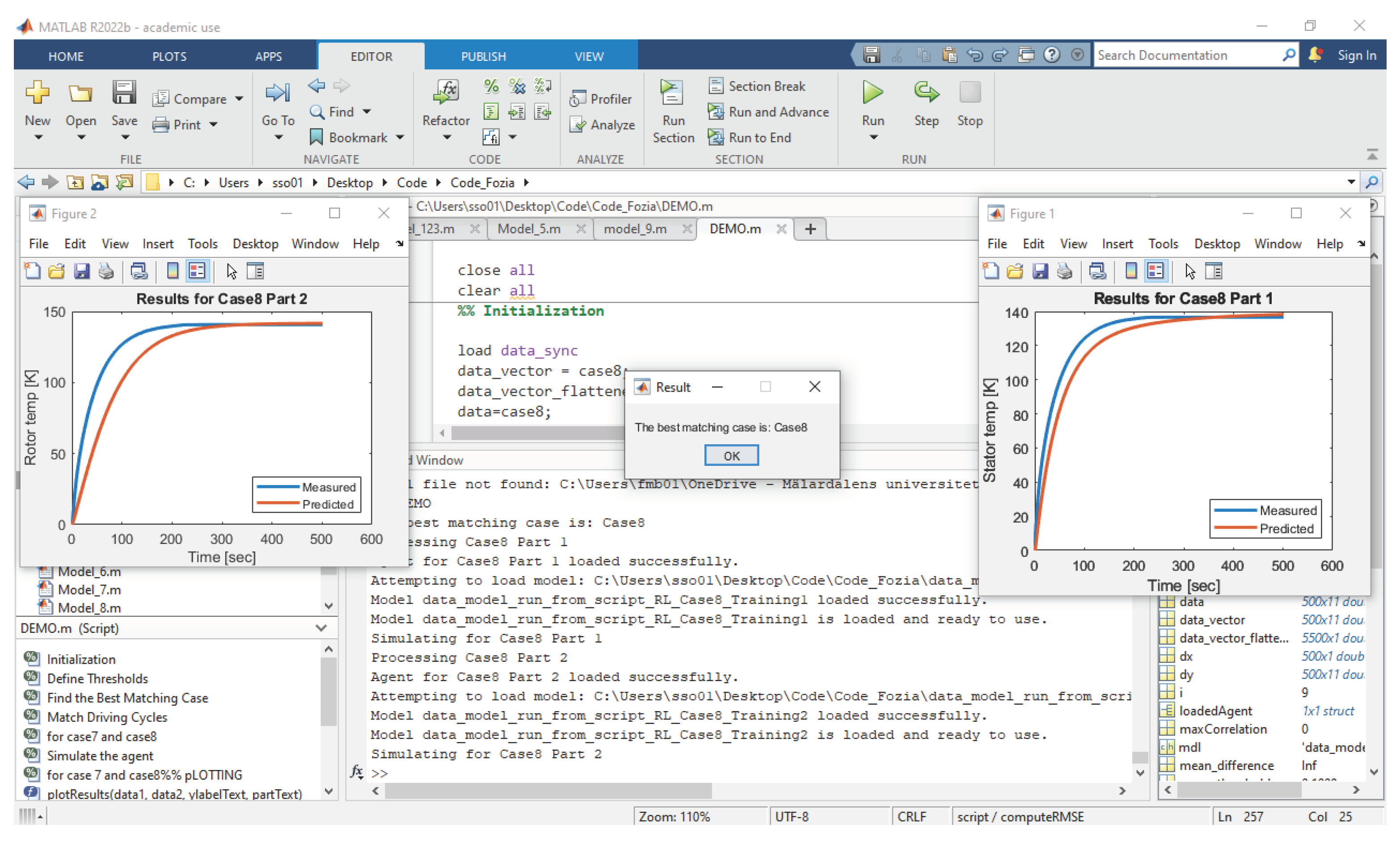
The proposed offline prediction strategy enhances efficiency by applying the pretrained models to known driving cycles data and adapting to new controller driving cycles data through additional training. The approach uses statistical methods like mean, standard deviation, correlation, and frequency analysis to match new driving cycles with previously encountered ones. The analysis is performed on the basis of data from the same type of induction motor. When new cycle data closely resembles stored cycles data, the system selects an appropriate pretrained model for temperature prediction as shown in Figure 6. This will save computational time and resources by avoiding further training. However, if the new driving cycle appears unique, the RL agent begins training with this new controller driving cycles data. This adaptive approach ensures that the model continuously evolves and learns from new motor usage patterns.

4. Results & Discussion

4.1. Preprocessing the Dataset

In this study, tool data from nine different driving cycles and measured data of one driving cycles data were employed to simulate an environment unknown to the agent. This facilitates the training process focused on identifying optimal thermal conductance parameters λ1s, λ2s, λ1r, and λ2r.

4.2. Training the RL Agents

The training parameters which are crucial for the learning process of RL agents are outlined across multiple tables, each focusing on distinct driving cycles. This detailed breakdown of training parameters highlights the strategic and customized approach for training the RL agents.
Table 1 presents the parameters for the Twin Delayed Deep Deterministic Policy Gradient (TD3) algorithm that is applied to driving cycles DC1, DC2, and DC3, specifying a limit of ten episodes, with each episode consisting of up to 600 steps.
Table 2 describes the training parameters relevant to the Deep Deterministic Policy Gradient (DDPG) algorithm used for driving cycles DC6, DC7, and DC4. Table 2 outlines a more detailed parameter set for the DDPG algorithm for predicting rotor and stator temperatures from driving cycle DC9. Both components are trained over 1000 episodes with a sample time of 0.1 seconds but differ in the maximum steps per episode, averaging window lengths, and stop values.
Table 3 specifies the training parameters for the DDPG algorithm for driving cycle DC9, closely following the stator's configuration in driving cycle DC8. This includes 1000 maximum episodes, 20 steps per episode, an averaging window of 50, a stop value of -740, and a sample time of 0.1 seconds.

4.3. Validating the Trained Agents

The validation of the RL agent involves regularly evaluating the policy it implements in the actual environment. The results of this process, in which it compares the observed and predicted temperatures for tool and measured driving cycles, are shown in the following figures.
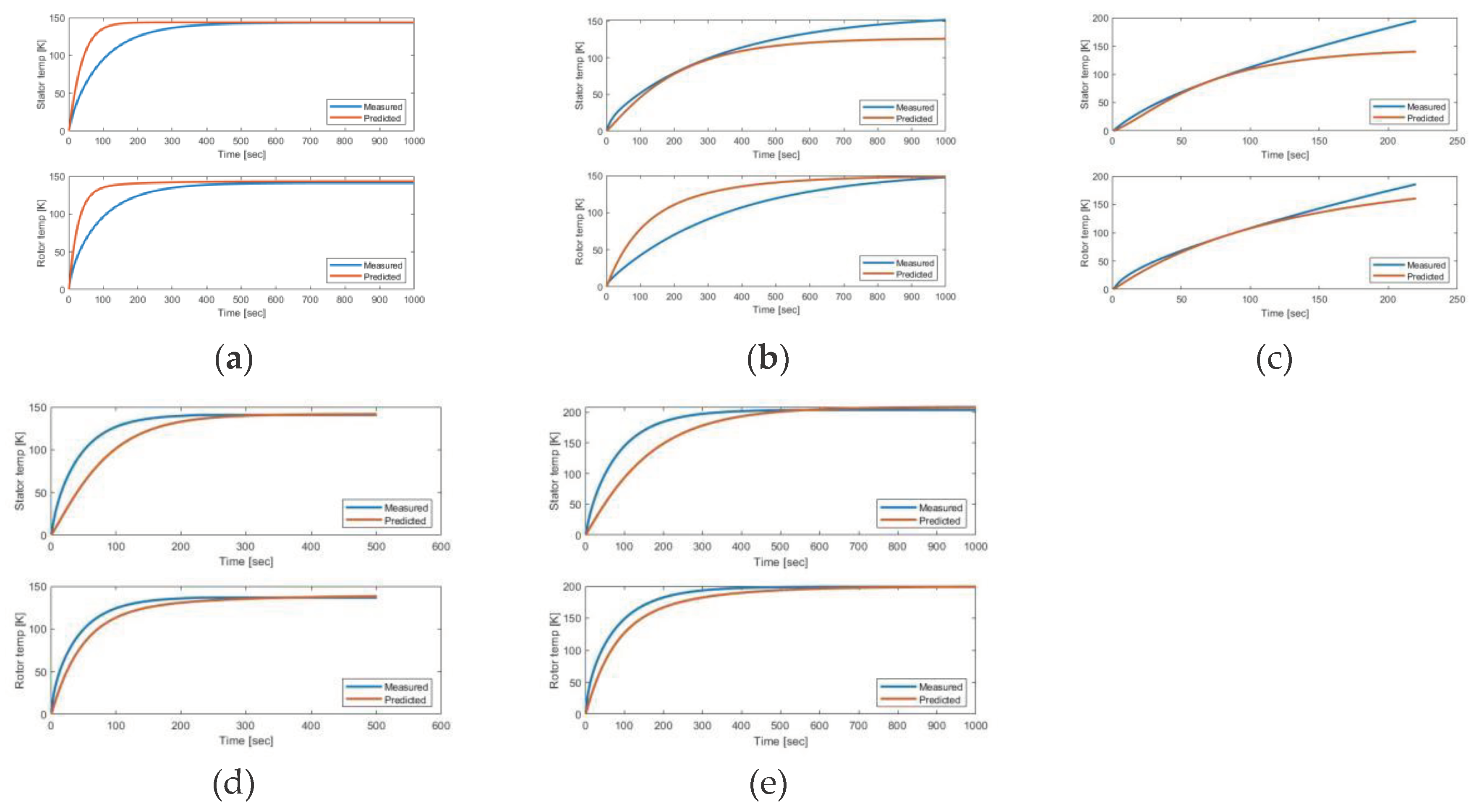
Figure 7 presents the outcomes from deploying a Twin Delayed Deep Deterministic Policy Gradient (TD3) reinforcement learning agent for temperature predictions across three specific driving cycles. This figure shows the temperature predictions over time for the stator and the rotor of an induction motor from tool data. In Figure 7, a blue line represents the actual measured temperature data, and an orange line shows the predicted temperature by the TD3 agent. The close match between measured data and the predictions made by the agents in three DC data indicate that the TD3 agent successfully learns and accurately estimates the thermal dynamics of induction motors. Furthermore, the precision of temperature prediction demonstrates the agent’s capability to generalize well from the training data.
Figure 8 displays the stator and rotor temperature predictions of the Deep Deterministic Policy Gradient (DDPG) reinforcement learning agent on five distinct driving cycles data labeled as cycles DC4, DC6, DC7, DC8 and DC9. Figure 8 depicts the DDPG agent’s pre-diction capabilities in aligning its temperature predictions closely with the actual data over time. Additionally, detailed insights highlight that the rotor temperature prediction of DC 6 and stator temperature prediction of DC7 were not accurate as still there was room for improvement and fine-tuning of the deep neural network is required to get approximate predictions from both driving cycles data.
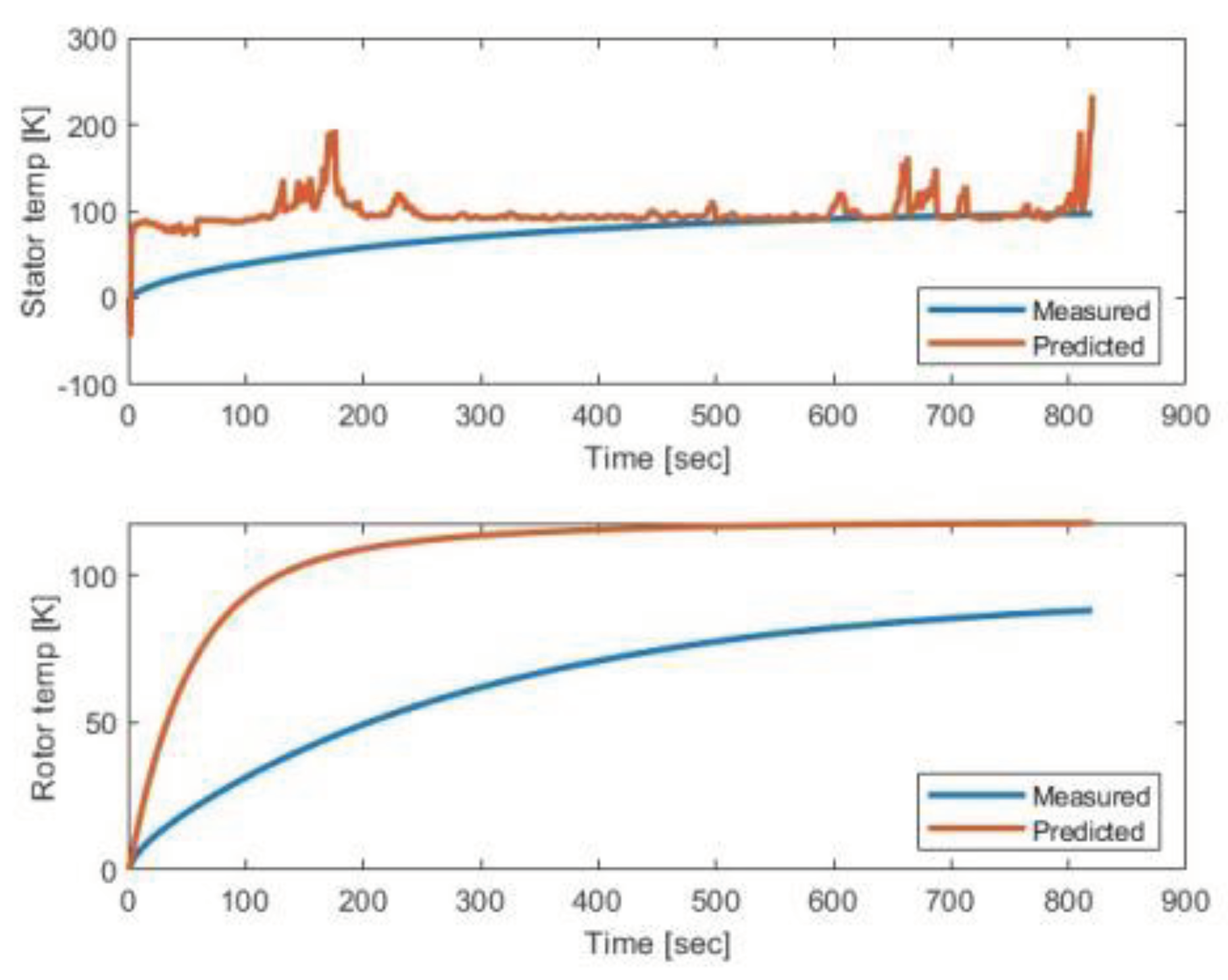
Figure 9 illustrates the performance of a predictive model for DC5 stator and rotor temperatures using SAC RL agent. TD3, DDPG agents were employed to get the optimal thermal parameters and temperature predictions from DC5. However, the SAC agent only provides improved temperature predictions for the stator, while it struggles to achieve accurate predictions for the rotor temperature. Figure 9 highlights the fluctuations and spikes in model predictions for stator temperature and indicates a less predictive accuracy of the model in case rotor temperature prediction. Optimization is required for DC5 for the thermal management and operational efficiency of electric motors.
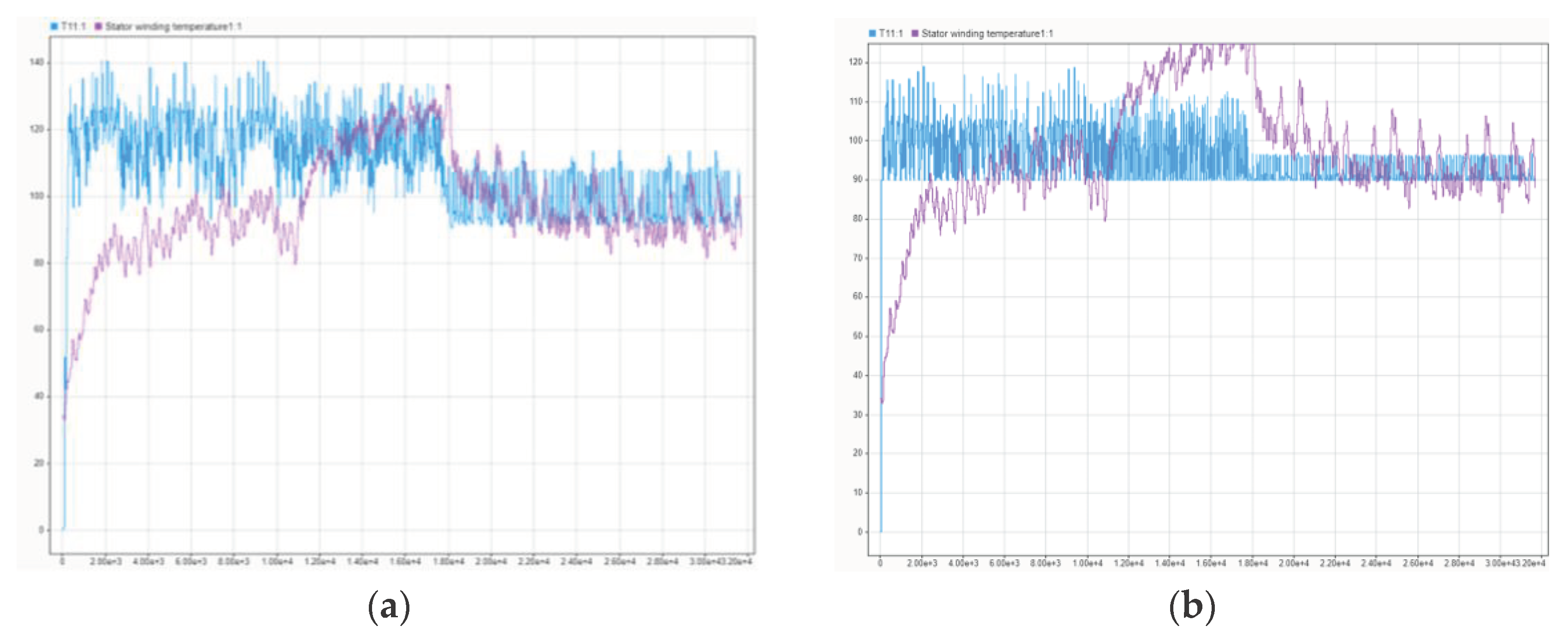
Figure 10 depicts the predicted stator winding temperatures from the measured data. SAC agent was employed for stator winding temperature prediction with and without the inclusion of airflow information. The prediction of stator temperature in the first figure, which includes airflow, displays more precise predictions of operating conditions. Whereas the second figure represents the predicted temperatures without considering the air-flow information. The absence of airflow data in the thermal model results in less accurate predictions, in which the agent is unable to capture the immediate effects of varying stator temperature. Adding airflow information to the proposed thermal models matters because it affects the prediction of stator winding temperature.

5. Conclusions

The paper presents a data-driven multi-agent reinforcement learning approach to parametrize a thermal model of an induction traction motor from recorded driving cycles. The trained reinforcement learning agents demonstrated good proficiency in devising strategies for managing thermal behaviors under different operational conditions. In offline mode, pre-trained models are utilized to predict the temperature from several driving cycles data. The integration of statistical techniques and clustering to identify relevant driving cycles for offline prediction further emphasizes the comprehensive nature of the approach. However, there are a few limitations of the proposed approach that the training of RL multi-agents can be computationally intensive and requires further investigation to generalize across different motor types and conditions.

Author Contributions

Conceptualization and methodology, F.F., A.F. and S.S.; software, F.M. and A.F.; validation, F.M.; data curation, S.S.; writing—original draft preparation, F.M.; writing—review and editing, A.F. and S.S. All authors have read and agreed to the published version of the manuscript.

Data Availability Statement

The driving cycles data is unavailable due to confidentiality agreements.

Acknowledgments

We gratefully acknowledge the support for this research provided by the AIDOaRt project, which is financed by the ECSEL Joint Undertaking (JU) under grant agreement No 101007350.

Conflicts of Interest

The authors declare no conflicts of interest.

Appendix A. Parametrizing the Thermal Model

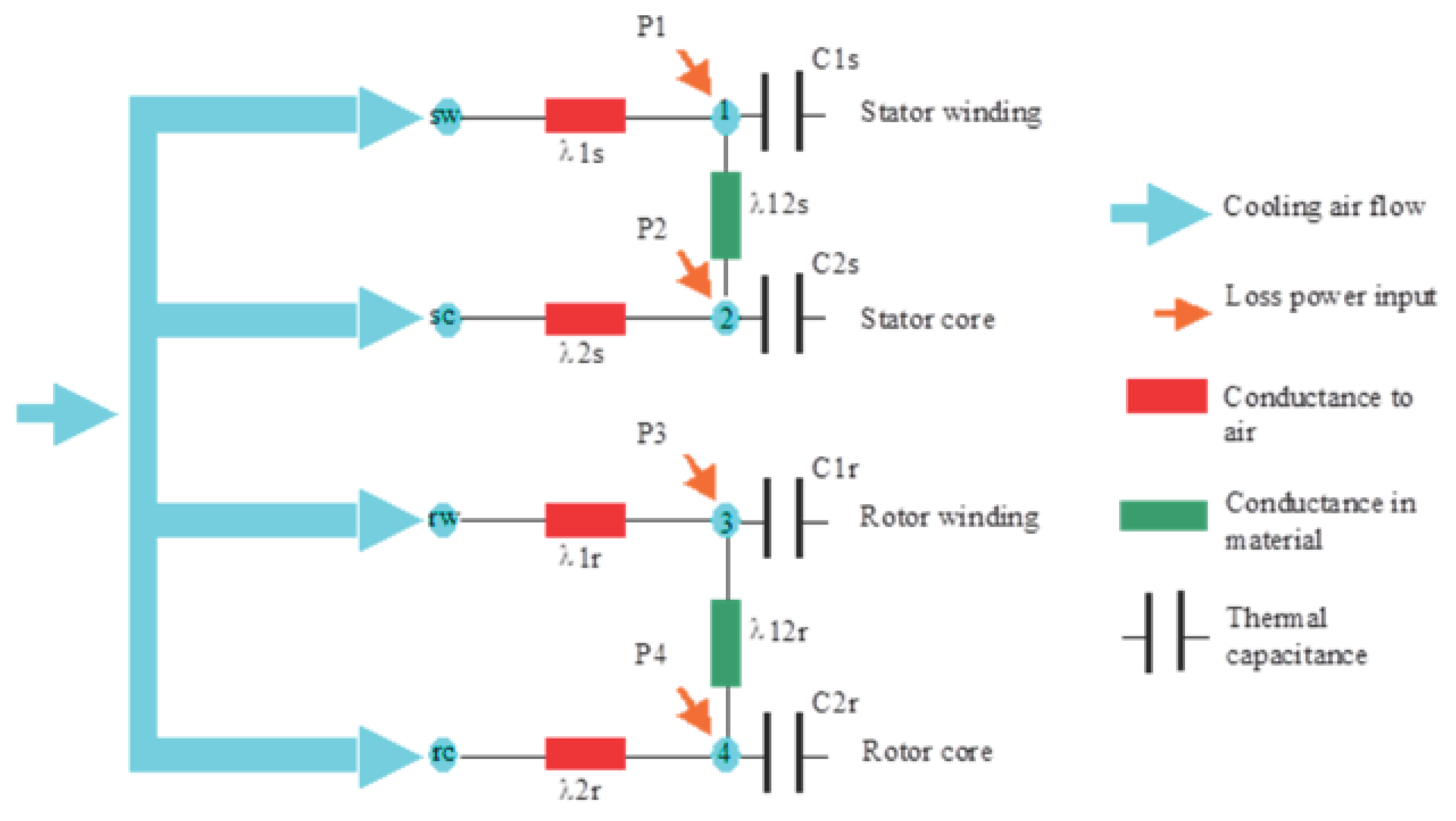
From a thermal point of view, the motor is modeled with four nodes: stator winding (node 1), stator core (node 2), rotor winding (node 3) and rotor core (node 4). The thermal equivalent network is illustrated in Figure A1 with thermal capacitances, to which a power source is connected and with thermal conductance among the nodes and to the cooling air.
Figure A1. Lumped parameter thermal network model.
Preprints 100313 g0a1
Thermal capacitance C 1 s , C 2 s , C 1 r , and C 2 r values are calculated analytically from the geometry and material information of the motor. The capacitance for stator yoke C 1 s is the sum of the capacitance of stator housing, stator back iron, stator tooth and flange mounted. The stator winding capacitance C 2 s includes the capacitance for the stator winding and the end winding capacitances. The capacitance for stator yoke C 1 r is the sum of the capacitance of rotor yoke, and rotor bars. The rotor winding capacitance C 2 r includes the capacitance for the rotor winding and the end winding capacitances The thermal conductance λ1s, λ2s, λ1r, λ2r vary with the airflow due to the convection. The model shown in Error! Reference source not found. can be represented mathematically by the following first-order differential system:
P 1 = C 1 s d T 1 dt + λ 1 s T 1 T env + λ 12 s T 1 T 2 ,
P 2 = C 2 s d T 2 dt + λ 2 s T 2 T env + λ 12 s T 2 T 1 ,
P 3 = C 1 r d T 3 dt + λ 1 r ( T 3 T env ) + λ 12 r ( T 3 T 4 ) ,
P 4 = C 2 r d T 4 dt + λ 2 r ( T 4 T env ) + λ 12 r ( T 4 T 3 ) ,
where Ti is the temperature at the corresponding node i. The temperatures of the cooling air at the four nodes (marked as sw, sc, rw and rc in Error! Reference source not found.) are assigned to the environment (or ambient) temperature T env .
The losses at the four nodes in Error! Reference source not found. are distributed as shown in Table A1 and they can be calculated as follows:
P 1 = K s t e m p P c u 1 + K s t r a y P s t r a y + K h a r m P h a r m ,
P 2 = K P f e P f e ,
P 3 = K r t e m p P c u 2 + ( 1 K s t r a y ) P s t r a y + ( 1 K h a r m ) P h a r m ,
P 4 = ( 1 K P f e ) P f e ,
where P c u 1 , P c u 2 , P s t r a y , P h a r m , P f e are the stator copper loss, rotor copper loss, stray loss, harmonic loss, and iron loss respectively. The coefficients K s t e m p , K r t e m p , K s t r a y , K h a r m and K P f e are the corresponding loss coefficients.
Table A1. Distribution of losses in the LPTN model.
Node Winding Losses Stray Losses Harmonic Losses Iron Losses
1 x x x
2 x
3 x x x
4 x
The losses in Equations A5-A8 can be calculated as follows [23,24,25,26]:
P c u 1 = R 1 I 1 2 ,
P c u 2 = R 21 I 21 2 ,
P s t r a y = P S U P f f n o m 1.5 I 1 I 1 , n o m   2 ,
P f e = K f   f α B m a x β ,
where I 1 , I 21 are the stator and rotor currents respectively, R1 and R21 are the stator and rotor winding resistances respectively which depend on the temperature according to the following equations:
R 1 = R 1,20 ( 1 + α R 1 ( T 1 20 ) ,
R 21 = R 21,20 ( 1 + α R 2 ( T 3 20 ) ,
where R 1,20 , R 21,20 are the stator and rotor winding resistance at 20 °C and α R 1 , α R 21 the temperature coefficient of stator and rotor, respectively. In Equation A11, f is the stator frequency with a nominal value fnom, I1 is the stator current with a nominal value I1,nom and PSUP is the equivalent rated input power. In Equation A12, Kf is a constant that depends on the material properties and the core geometry, f is the frequency of the magnetic field, Bmax is the peak magnetic flux density in the core and α and β are empirically determined constants. The harmonic losses P h a r m o are measured at a few operation points and included as a look-up table in the loss model.

References

  1. Fathy Abouzeid, A.; Guerrero, J.M.; Endemaño, A.; Muniategui, I.; Ortega, D.; Larrazabal, I.; Briz, F. Control strategies for induction motors in railway traction applications. Energies 2020, 13, 700. [Google Scholar] [CrossRef]
  2. Kirchgässner, W.; Wallscheid, O.; Böcker, J. Data-driven permanent magnet temperature estimation in synchronous motors with supervised machine learning: A benchmark. IEEE Transactions on Energy Conversion 2021, 36, 2059–2067. [Google Scholar] [CrossRef]
  3. Zhang, Y.; Huang, J.; He, L.; Zhao, D.; Zhao, Y. Reinforcement learning-based control for the thermal management of the battery and occupant compartments of electric vehicles. Sustain. Energy Fuels 2024, 8, 588–603. [Google Scholar] [CrossRef]
  4. Hannan, M.A.; Ali, J.A.; Mohamed, A.; Hussain, A. Optimization techniques to enhance the performance of induction motor drives: A review. Renew. Sustain. Energy Rev. 2018, 81, 1611–1626. [Google Scholar] [CrossRef]
  5. Ramakrishnan, R. , Islam, R., Islam, M. and Sebastian, T. (2009) 'Real time estimation of parameters for controlling and monitoring permanent magnet synchronous motors', 2009 IEEE International Electric Machines and Drives Conference. pp. 1194–1199.
  6. Wilson, S.D.; Stewart, P.; Taylor, B.P. Methods of resistance estimation in permanent magnet synchronous motors for real-time thermal management. IEEE Trans. Energy Convers. 2010, 25, 698–707. [Google Scholar] [CrossRef]
  7. Wallscheid, O. Thermal monitoring of electric motors: State-of-the-art review and future challenges. IEEE Open J. Ind. Appl. 2021, 2, 204–223. [Google Scholar] [CrossRef]
  8. Dorrell, D.G. Combined thermal and electromagnetic analysis of permanent-magnet and induction machines to aid calculation. IEEE Trans. Ind. Electron. 2008, 55, 3566–3574. [Google Scholar] [CrossRef]
  9. Sciascera, C.; Giangrande, P.; Papini, L.; Gerada, C.; Galea, M. Analytical thermal model for fast stator winding temperature prediction. IEEE Trans. Ind. Electron. 2017, 64, 6116–6126. [Google Scholar] [CrossRef]
  10. Zhu, Y. , Xiao, M., Lu, K., Wu, Z. and Tao, B. A simplified thermal model and online temperature estimation method of permanent magnet synchronous motors. Appl. Sci. 2019, 9, 3158. [Google Scholar] [CrossRef]
  11. Guemo, G. G. , Chantrenne, P. and Jac, J. (2013) 'Parameter identification of a lumped parameter thermal model for a permanent magnet synchronous machine', 2013 International Electric Machines & Drives Conference. pp. 1316-132.
  12. Huber, T., W. Peters and J. Böcker (2014) 'Monitoring critical temperatures in permanent magnet synchronous motors using low-order thermal models', 2014 International Power Electronics Conference (IPEC-Hiroshima 2014-ECCE ASIA), IEEE.
  13. Xiao, S. and Griffo, A. Online thermal parameter identification for permanent magnet synchronous machines. IET Electr. Power Appl. 2020, 14, 2340–2347. [Google Scholar] [CrossRef]
  14. Gedlu, E. G. , Wallscheid, O. and Böcker, J. (2020) 'Permanent magnet synchronous machine temperature estimation using low-order lumped-parameter thermal network with extended iron loss model', The 10th International Conference on Power Electronics, Machines and Drives (PEMD 2020). IET.
  15. Wallscheid, O. Thermal monitoring of electric motors: State-of-the-art review and future challenges. IEEE Open J. Ind. Appl. 2021, 2, 204–223. [Google Scholar] [CrossRef]
  16. Kirchgässner, W. , Wallscheid, O. and Böcker, J. (2019) 'Deep residual convolutional and recurrent neural networks for temperature estimation in permanent magnet synchronous motors', 2019 IEEE International Electric Machines & Drives Conference (IEMDC). IEEE.
  17. Zhu, Y.; Xiao, M.; Lu, K.; Wu, Z.; Tao, B. A simplified thermal model and online temperature estimation method of permanent magnet synchronous motors. Appl. Sci. 2019, 9, 3158. [Google Scholar] [CrossRef]
  18. Wlas, M.; Krzeminski, Z.; Toliyat, H.A. Neural-network-based parameter estimations of induction motors', IEEE Trans. Ind. Electron. 2008, 55, 1783–1794. [Google Scholar] [CrossRef]
  19. Kirchgässner, W.; Wallscheid, O.; Böcker, J. Thermal neural networks: lumped-parameter thermal modeling with state-space machine learning. Eng. Appl. Artif. Intell. 2023, 117, 105537. [Google Scholar] [CrossRef]
  20. Book, G. , Traue, A., Balakrishna, P., Brosch, A., Schenke, M., Hanke, S., Kirchgässner, W. and Wallscheid, O. Transferring online reinforcement learning for electric motor control from simulation to real-world experiments. IEEE Open J. Power Electron. 2021, 2, 187–201. [Google Scholar] [CrossRef]
  21. Zhang, Q.; Zeng, W.; Lin, Q.; Chng, C.B.; Chui, C.K.; Lee, P.S. Deep reinforcement learning towards real-world dynamic thermal management of data centers. Appl. Energy 2023, 333, 120561. [Google Scholar] [CrossRef]
  22. Fattouh, A.; Sahoob, S. Data-driven reinforcement learning-based parametrization of a thermal model in induction traction motors. Scand. Simul. Soc. 2023, 310–317. [Google Scholar]
  23. Kral, C.; Haumer, A.; Lee, S.B. A practical thermal model for the estimation of permanent magnet and stator winding temperatures. IEEE Trans. Power Electron. 2013, 29, 455–464. [Google Scholar] [CrossRef]
  24. Maroteaux, A. (2016) 'Study of analytical models for harmonic losses calculations in traction induction motors', KTH, School of Electrical Engineering (EES).
  25. Nasir, B.A. An Accurate Iron Core Loss Model in Equivalent Circuit of Induction Machines. J. Energy 2020, 2020, 1–10. [Google Scholar] [CrossRef]
  26. IEC/TS 60349-3 (2010) 'Electric traction - Rotating electrical machines for rail and road vehicles - Part 3: Determination of the total losses of converter-fed alternating current motors by summation of the component losses'.
  27. Wallscheid, O.; Böcker, J. Global identification of a low-order lumped-parameter thermal network for permanent magnet synchronous motors. IEEE Trans. Energy Convers. 2015, 31, 354–365. [Google Scholar] [CrossRef]
Figure 1. The reinforcement learning framework (adopted from [22], see Appendix A for terminologies and equations).
Preprints 100313 g001
Figure 2. The architecture of the TD3 agent.
Preprints 100313 g002
Figure 3. The architecture of the DDPG agent.
Preprints 100313 g003
Figure 4. The architecture of the SAC agent.
Preprints 100313 g004
Figure 5. The training process of: (a) TD3; (b) DDPG; (c) SAC agents.
Preprints 100313 g005
Figure 6. Statistical estimation, matching and loading of the pre-trained models.
Preprints 100313 g006
Figure 7. Results of the driving cycles (DCs): (a) DC1; (b) DC2; (c) DC3 using the TD3 agent.
Preprints 100313 g007
Figure 8. Results of the driving cycles (DCs): (a) DC4; (b) DC6; (c) DC7; (d) DC8; (e) DC9 using the DDPG agent.
Preprints 100313 g008
Figure 9. Results of the driving cycle DC5 using the SAC agent.
Preprints 100313 g009
Figure 10. Results of driving cycles of measured data using the SAC agent: (a) with airflow information; (b) without airflow information.
Preprints 100313 g010
Table 1. Training parameters of TD3 agent for driving cycles DC1, DC2 and DC3.
Property Value
max episodes 10
max steps per episodes 600
average window length 500
stop training value -10
agent sample time 0.1 s
Table 2. Training parameters of DDPG agent for driving cycles DC4, DC6 and DC7.
Property Value (DC4, DC7, DC7) Value (DC9)
max episodes 1000 1000
max steps per episodes 600 20
average window length 500 20
stop training value -10 -740
agent sample time 0.1 s 0.1 s
Table 3. Training parameters of DDPG agent for driving cycles DC8.
Property Value (rotor) Value (stator)
max episodes 1000 1000
max steps per episodes 600 20
average window length 500 50
stop training value -10 -740
agent sample time 0.1 s 0.1 s
Disclaimer/Publisher’s Note: The statements, opinions and data contained in all publications are solely those of the individual author(s) and contributor(s) and not of MDPI and/or the editor(s). MDPI and/or the editor(s) disclaim responsibility for any injury to people or property resulting from any ideas, methods, instructions or products referred to in the content.
Copyright: This open access article is published under a Creative Commons CC BY 4.0 license, which permit the free download, distribution, and reuse, provided that the author and preprint are cited in any reuse.
Prerpints.org logo

Preprints.org is a free preprint server supported by MDPI in Basel, Switzerland.

Subscribe

© 2024 MDPI (Basel, Switzerland) unless otherwise stated