1. Introduction
Mental health is a serious issue. For the past few years, a non-profit organization, Open Sourcing Mental Health (OSMH) has been publishing the results of its survey on mental health of employees primarily in the tech / IT industry under Creative Commons Attribution-ShareAlike 4.0 International license. The literature survey shows that the dataset [
1] is popular among the researchers. Multiple articles have used machine learning models on the dataset(s) to draw valuable insights. The models were treated as black boxes, assessed using the conventional evaluation metrics and concluded to have performed significantly well. However, no attempts have been made to gauge the reliability of the results. LIME [
2] and SHAP [
3] have become popular tools for enhancing the transparency and accountability of machine learning models, enabling users to gain insights into their decision-making processes and build trust in their predictions. Both approaches aim to unravel the underlying logic driving the models’ predictions, particularly for individual data points. We therefore attempted to use them to see how reliable the models were in their prognosis.
Our experiments in trying to justify the results using LIME [
2] and SHAP [
3] show that the class predictions relied significantly on unsound weights for features in the dataset. The experiments demonstrate the need to supplement the conventional metrics with explanation of the model behavior and justification of the results. The work aims to answer the following research questions:
RQ1: How reliable are the evaluation metrics such as accuracy in assessing the machine learning model performance in making important predictions?
RQ2: How well do the explainable AI techniques, SHAP and LIME complement the conventional evaluation metrics?
RQ3: How do the various machine learning algorithms compare when it comes to the explainability of their outcomes?
A brief review of the current literature follows. A search for "Mental Health in Tech Survey" in Google Scholar shows scores of articles that apparently have used the OSMH datasets. A few of them [
4] [
5] applied machine learning to predict the mental health of employees mainly working in the tech / IT sector. One of them [
6] attempted to interpret the model using SHAP and Permutation Importance but no conclusions were drawn. Even according to their analysis, past mental health disorders and "whether it would interfere with work if treatment is not effective" weighed more than "whether it has been professionally diagnosed," which does not make much sense. Generalized Linear Models applied to the dataset show a high correlation between mental health issues and working for a primarily technology-oriented company combined with certain demographics [
7].
Prior work on Linear Regression, Multi-Layer Perceptron, and Echo State Network shows that there is a close relationship between the SHAP values and the differences in the performance of the models [
8]. Since the models differ in complexity, the paper concludes that model complexity is an important consideration concerning explainability. The metrics used in the work are Monotonicity, trendability, and prognosability. There has been an attempt to measure the effectiveness of explainable techniques like SHAP and LIME [
9]. The authors created a new methodology to evaluate precision, generality, and consistency in attribution methods. They found that both SHAP and LIME lacked in all three of these qualities, leading to the conclusion that more investigation is needed in the area of explainability. In this context, it is also worth mentioning about the explainable AI (XAI) toolkit [
10] that is built on top of DARPA’s efforts in XAI. The toolkit is purported to be a resource for everyone wanting to use AI responsibly.
Explainability and fairness have been recommended for AI models used in healthcare in what the authors call "the FAIR principles" [
11]. Understandably, recent literature has abundant work in these growing areas. Classification and explainability were attempted on publicly available English language datasets related to mental health [
12]. The focus of the work is in analyzing the spectrum of language behavior evidenced on social media. Interestingly, t-SNE and UMAP have also been considered as explainable artificial intelligence (XAI) methods in a survey of the current literature on explainability of AI models in medical health [
13]. Explainable AI (XAI) continues to be a hot area of research particularly in the health domain as can be observed from the recent literature [
14] [
15]. Machine learning models deployed in the health domain can suffer from fairness issues too and some of the methods to address fairness can degrade the model’s performance in terms of accuracy and fairness as well [
16].
In an interesting scenario, SHAP explanations were used as features to improve machine learning classification [
17]. The article discusses the cost of wrong predictions in finance and how SHAP explanations can be used to reduce this cost. The authors propose a two-step classification process where the first step uses a base classifier and the second step uses a classifier trained on SHAP explanations as new features. They test their method on nine datasets and find that it improves classification performance, particularly in reducing false negatives.
However, SHAP and LIME are vulnerable to adversarial attacks. In an article about fooling post hoc explanation methods for black box models [
18], the authors propose a new framework to create “scaffolded” classifiers that hide the biases of the original model. They show that these new classifiers can fool SHAP and LIME into generating inaccurate explanations. A recent detailed survey [
19] on explainable AI (XAI) methods brought out their limitations, including those of LIME. In yet another recent survey on XAI methods, including LIME and SHAP, for use in the detection of Alzheimer’s disease [
20], the authors too brought out the limitations and open challenges with XAI methods. A number of open issues with XAI have been discussed under 9 categories providing research directions in a recently published work [
21].
1.1. Contribution
Our literature survey brought out the advantages and disadvantages of explainability techniques. Despite the limitations of SHAP and LIME described above, this work successfully uses them to show how the black box approach of using machine learning algorithms can be dangerously misleading. For instance, our experiments show that with a significant accuracy and a 100% prediction probability, the machine learning model called SGD Classifier may predict a person not have a mental health condition even when they answered "sometimes" to the survey question, "If you have a mental health condition, do you feel that it interferes with your work?" In doing so, the model relies more on the fact that the person did not answer with a "often" or "rarely" to the same question than on the fact that the person did answer "sometimes." The very fact that the person answered this question implies that the person accepts they have a mental health condition. But the SGD Classifier predicts the person not to have a mental health condition. The prediction is therefore highly misleading. To the best of our knowledge, the work is unique in highlighting the inadequacy of the conventional evaluation metrics in assessing machine learning model performance in the mental health domain and argues strongly that the metrics need to be corroborated with a deeper understanding of the relationships between features and outcomes.
1.2. Paper organization
The remainder of the paper is organized as follows.
Section 2 describes the approach, detailing the dataset, tools, and the experiments. Results from the experiments are presented in
Section 3.
Section 4 discusses the results and presents the analysis. Finally, the conclusion is presented in
Section 5.
2. Materials and Methods
After performing some intuitive data preprocessing steps on the dataset such as dropping irrelevant columns like timestamps and comments, smoothing the outliers, and renaming the columns for consistency, class prediction is performed using a host of machine learning algorithms, which are all popularly used in the literature. The algorithms used are: Logistic Regression [
22], K-NN [
23], Decision Tree [
24], Random Forest [
25], Gradient Boosting [
26], Adaboost [
27], SGDClassifier [
28], Naive Bayes [
29], Support Vector Machines [
30], XGBoost [
31], and LightGBM [
32]. For brevity, the algorithms are not described here. Citations are provided instead. The selection of the algorithms was based on the existing literature [
4].
LIME (Local Interpretable Model-Agnostic Explanations) [
2] and SHAP (SHapley Additive exPlanations) [
3] are two prominent techniques used to demystify the complex workings of machine learning models. These are much better than merely computing feature importance using, say, information gain [
24]. For instance, features with more unique values tend to have higher information gain simply due to the increased opportunity for splits, even if their true predictive power is limited. Also, information gain only considers individual features and does not capture how features might interact with each other to influence the outcome. On the other hand, attribution methods like SHAP and LIME capture complex relationships between features and can identify synergistic effects. The results therefore are then attempted to be justified using the explainability algorithms, SHAP and LIME. Both SHAP and LIME are used for complementary insights. LIME excels at local explanations [
2], while SHAP provides global feature importance and theoretical guarantees [
3]. Details are provided below.
2.1. Dataset
The dataset used for the experiments in this work is called the "Mental Health in Tech Survey [
1]." The data is from a survey conducted in 2014 pertaining to the prevalence of mental health issues among individuals working in the technology sector. Some of the questions asked in the survey include whether the respondent has a family history of mental illness, how often they seek treatment for mental health conditions, and whether their employer provides mental health benefits among questions about demographics, work environment, job satisfaction, and other mental health-related factors. The class is determined by the answer to the question in the survey, "Have you ever been diagnosed with a mental health disorder?" and is used as the target variable for the experiments. For the data pre-processing, we dropped the timestamp, country, state, and comments because those columns contain a number of missing values and are not as relevant for the prediction of mental health. Also one of the numerical values named "Age" contains many outliers and missing values. Therefore we replaced those values with the median value for our experiment. The data is then split into training and test sets in a ratio of 0.7:0.3.
2.2. LIME: Local Interpretable Model-Agnostic Explanations
LIME [
2] is a technique used to explain individual predictions made by machine learning models that often are used as "black boxes." It is model agnostic and works with any type of model, regardless of its internal structure or training process. LIME provides explanations specific to a single prediction, rather than trying to interpret the model globally. This allows for capturing nuanced relationships between features and outcomes for individual data points. LIME explanations are formulated using human-understandable concepts, such as feature weights or contributions. This enables users to grasp why the model made a particular prediction without needing deep expertise in the model’s internal workings.
The core principle of LIME relies on surrogate models that are simple and interpretable like linear regression. Such a surrogate model is fitted to approximate the black box model’s behavior around the data point of interest. This is achieved through the following steps.
Generate perturbations: A set of perturbed versions of the original data point is created by slightly modifying its features. This simulates how changes in input features might affect the model’s prediction.
Query the black box: The model’s predictions for each perturbed data point are obtained.
Train the surrogate model: A local surrogate model, such as a linear regression, is fit to the generated data and corresponding predictions. This model aims to mimic the black box’s behavior in the vicinity of the original data point.
Explain the prediction: The weights or coefficients of the trained surrogate model represent the contributions of each feature to the model’s output. These weights are interpreted as the explanation for the original prediction.
The surrogate model can often be represented as
where
The weights then explain the model’s prediction, indicating how much each feature influenced the outcome. LIME uses various techniques to ensure the faithfulness of the explanation to the original model, such as regularization and weighting of perturbed points based on their proximity to the original data point.
2.3. SHAP: SHapley Additive exPlanations
SHAP [
3] is also a model-agnostic technique for explaining machine learning models by assigning each feature an importance value for a particular prediction. It provides both individual prediction explanations (local) and overall feature importance insights across the dataset (global). It applies Shapley values [
33] from coalitional game theory to calculate feature importance. In a game with players (features), a Shapley value represents a player’s average marginal contribution to all possible coalitions (subsets of features). SHAP analyzes how each feature’s marginal contribution impacts the model’s output, considering all possible feature combinations.
For a model f and an input instance x with features S = x1, x2, ..., xn, the SHAP value for a feature xi is defined as
where
represents the SHAP value for feature xi
S is a subset of features, S’ excluding xi
f(S) is the model’s prediction using only features in S
n is the number of features
can be considered as a weighing factor
As can be seen from the above equation, the marginal importance of each feature is computed by including and excluding the feature in the prediction. SHAP assumes an additive feature attribution model, but not in the units of prediction. Therefore, a "link function" is used for additivity.
where
Positive SHAP values indicate a feature pushing the prediction toward a higher value. Negative SHAP values indicate a feature pushing the prediction toward a lower value. Larger absolute SHAP values indicate greater feature importance for that prediction.
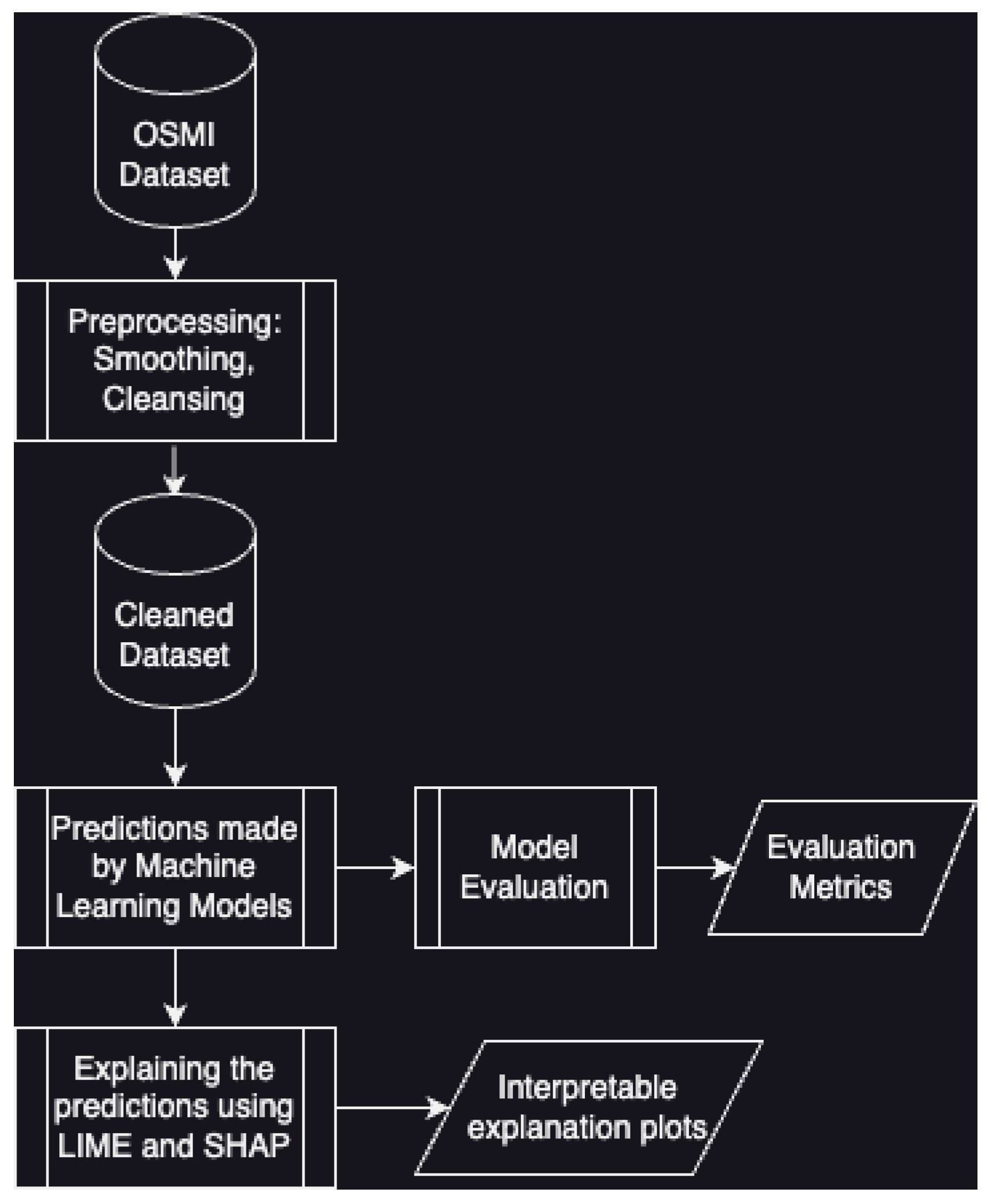
The methodology for the experiments is further described in
Figure 1. After preprocessing the data, various machine learning models are used to make predictions, and are evaluated using a number of metrics. The models are then passed as parameters to LIME and SHAP explainers to generate interpretable plots.
3. Results
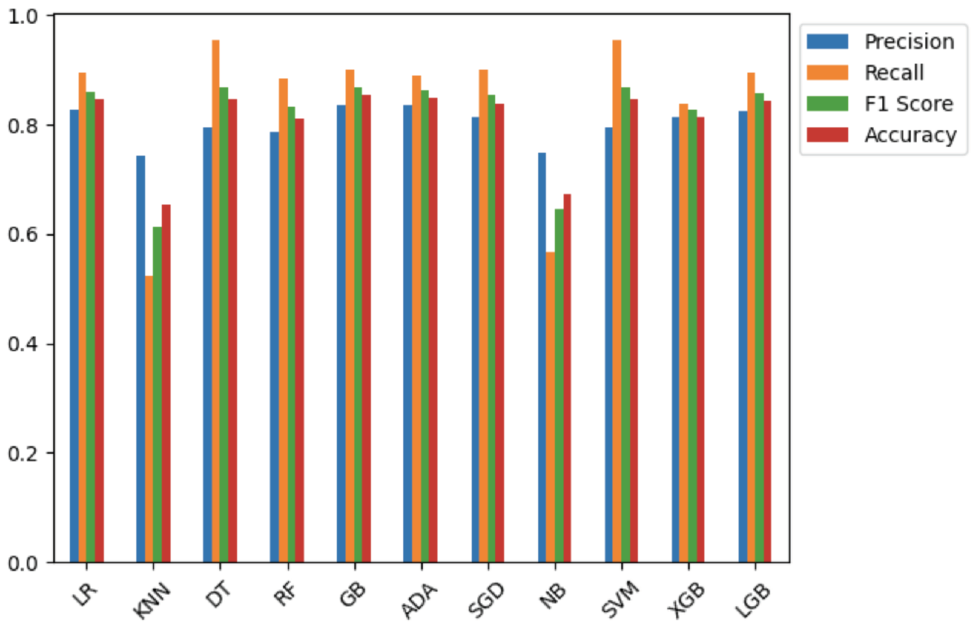
All the Python implementations of the machine learning algorithms used for prediction and the attribution methods, SHAP and LIME are imported and used with some fine-tuning of limited hyperparameters obtained by grid search. The classification results obtained are similar to the ones in the literature [
4] and are tabulated in
Table 1 and
Figure 2. To assess any impact due to class imbalance, we also compute the F1-score in addition to other metrics. The machine learning algorithms used for this work are the same as the ones used in [
4], which has been used as the baseline for comparison with our work.
The hyperparameters used with each of the models are summarized in
Table 2.
The specific findings from the application of SHAP and LIME on each of the models are discussed in the following subsections.
3.1. Logistic Regression
The evaluation metrics, Precision, Recall, F1 score, and Accuracy obtained from the application of logistic regression are tabulated in
Table 1.
3.1.1. Analysis of results SHAP and LIME
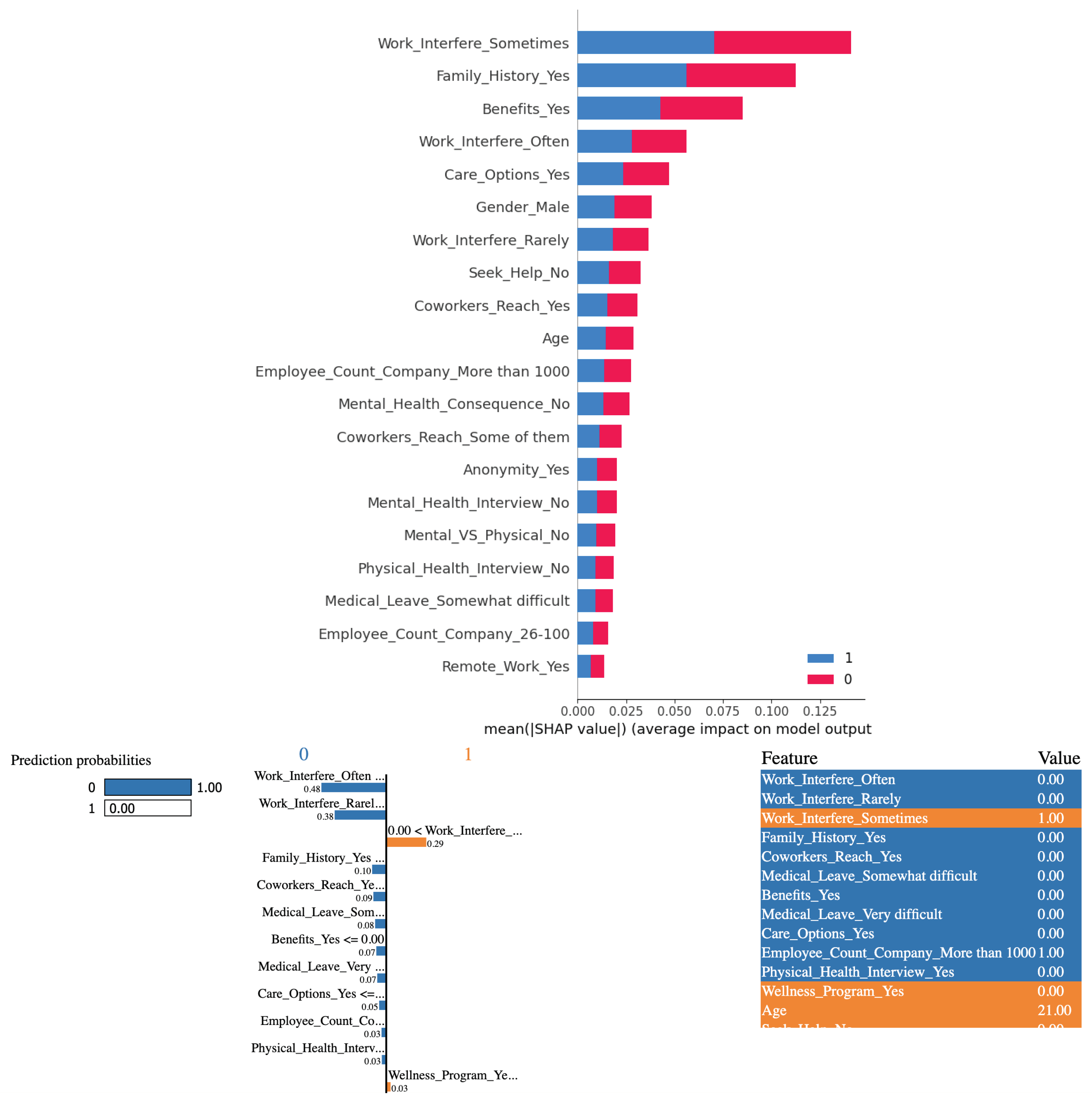
Based on the outcomes derived from employing logistic regression in conjunction with the SHAP and LIME methods, it is evident that the variable "Work Interference(Sometimes)" significantly influences the determination of mental health conditions among study participants.
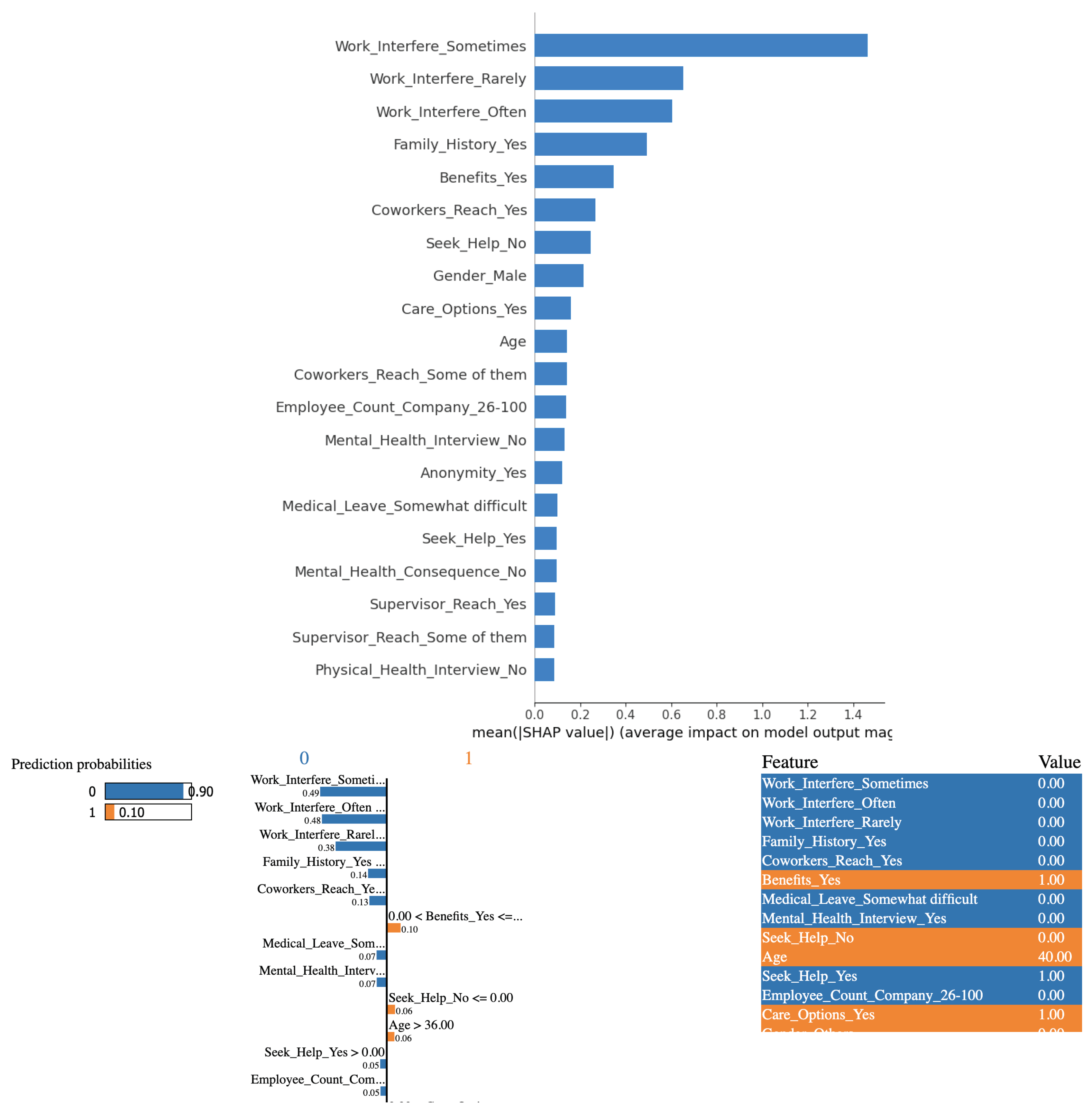
In
Figure 3(a) at the top, there are 3 charts. The leftmost is the predicted outcome. In this specific instance, the outcome is "no mental health issue with 90% certainty," indicated by the blue-colored bar. The rightmost chart is a listing of the feature-value pairs for the specific instance. Each feature in the middle plot is represented by a color-coded bar whose length (positive or negative) indicates its overall contribution to the prediction. Higher positive values imply the feature pushes the prediction toward the outcome of the corresponding color, while higher negative values imply it opposes it. For instance, the biggest factor that pushed the prediction to a "no" is in blue called "Work_Interfere_Sometimes" that corresponds to the survey question, "If you have a mental health condition, do you feel that it interferes with your work?" Interestingly, it played a more significant role in the model predicting "no" than Work_Interfere_Rarely, which is a fallacy. One would expect that if the mental health condition interferes less frequently or for that matter does not interfere less frequently, meaning never interferes, it would be a better predictor of the complete absence of mental health condition than if it interferes more frequently or does not interfere more frequently. The latter case implies that there is still a possibility that it still interferes once in a while. Hence the fallacy.
LIME is a local interpretation of a specific instance. SHAP on the other hand, offers both individual prediction explanations and overall feature importance insights. Individual plots tell why a specific prediction was made, while summary plots show the average impact of each feature across the entire dataset. Since individual plots were examined using LIME,
Figure 3(b) at the bottom shows the summary plot for a more comprehensive analysis. As can be seen, answering "sometimes" to the survey question, "If you have a mental health condition, do you feel that it interferes with your work?" weighs far more to the logistic regression model in predicting than answering "often" or "rarely," which is counter-intuitive. Similarly, an employer providing mental health benefits weighs more than the person’s demographics like age and gender. Despite these seeming anomalies, logistic regression achieves superlative evaluation metrics as can be seen from
Table 1.
3.2. Explanations based on the K-Nearest Neighbors Algorithm
Despite fine-tuning the hyperparameters, K-NN algorithm does not perform as well as logistic regression. The evaluation metrics, Precision, Recall, F1 score, and Accuracy obtained from the application of K-Nearest Neighbors algorithm are tabulated in
Table 1.
3.2.1. SHAP and LIME analysis of the K-NN model performance
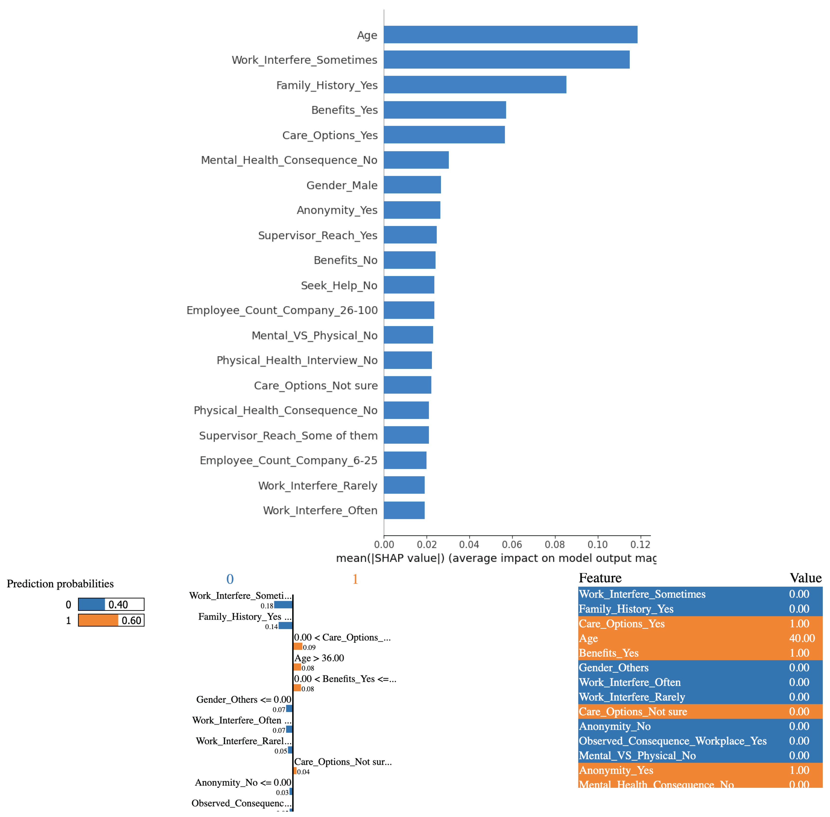
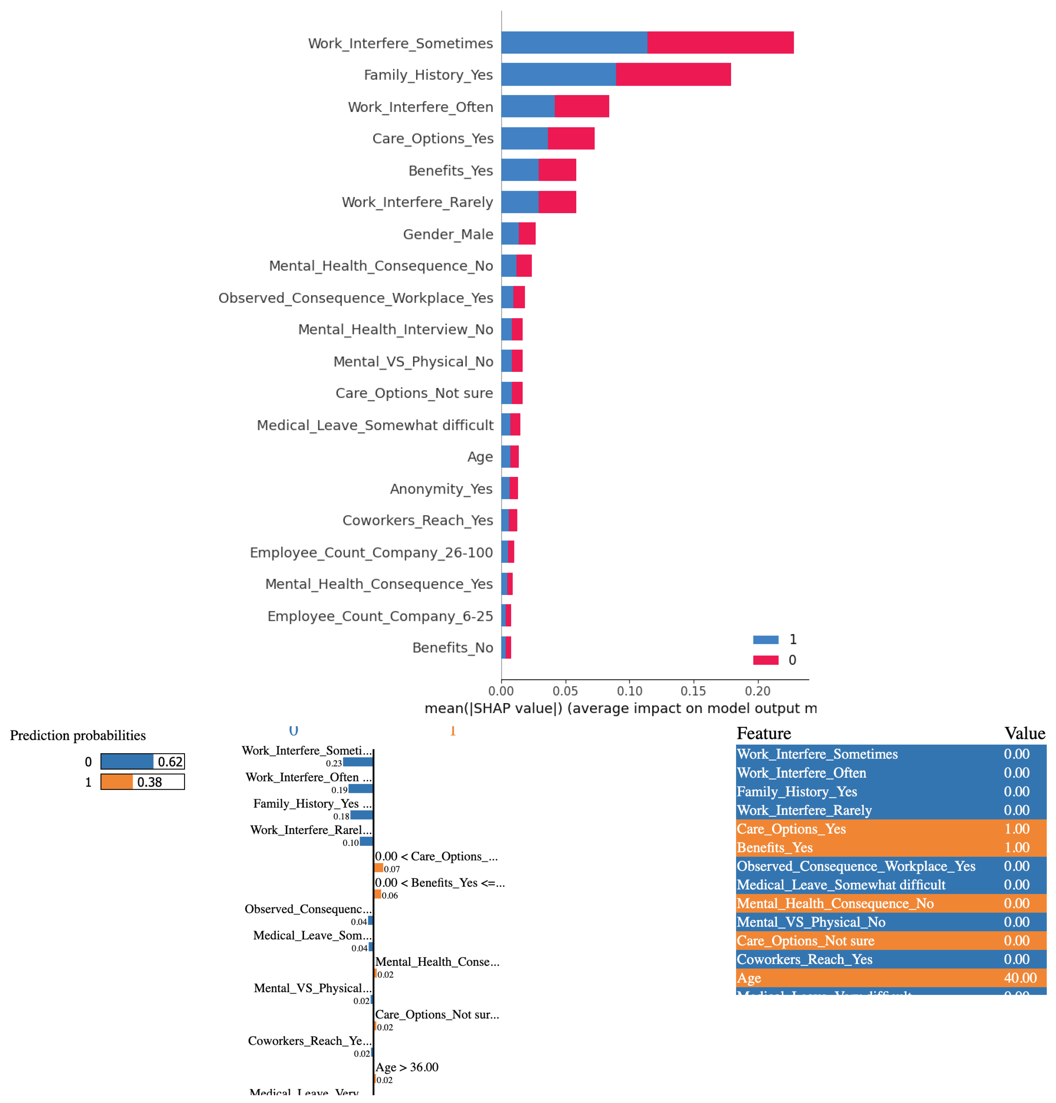
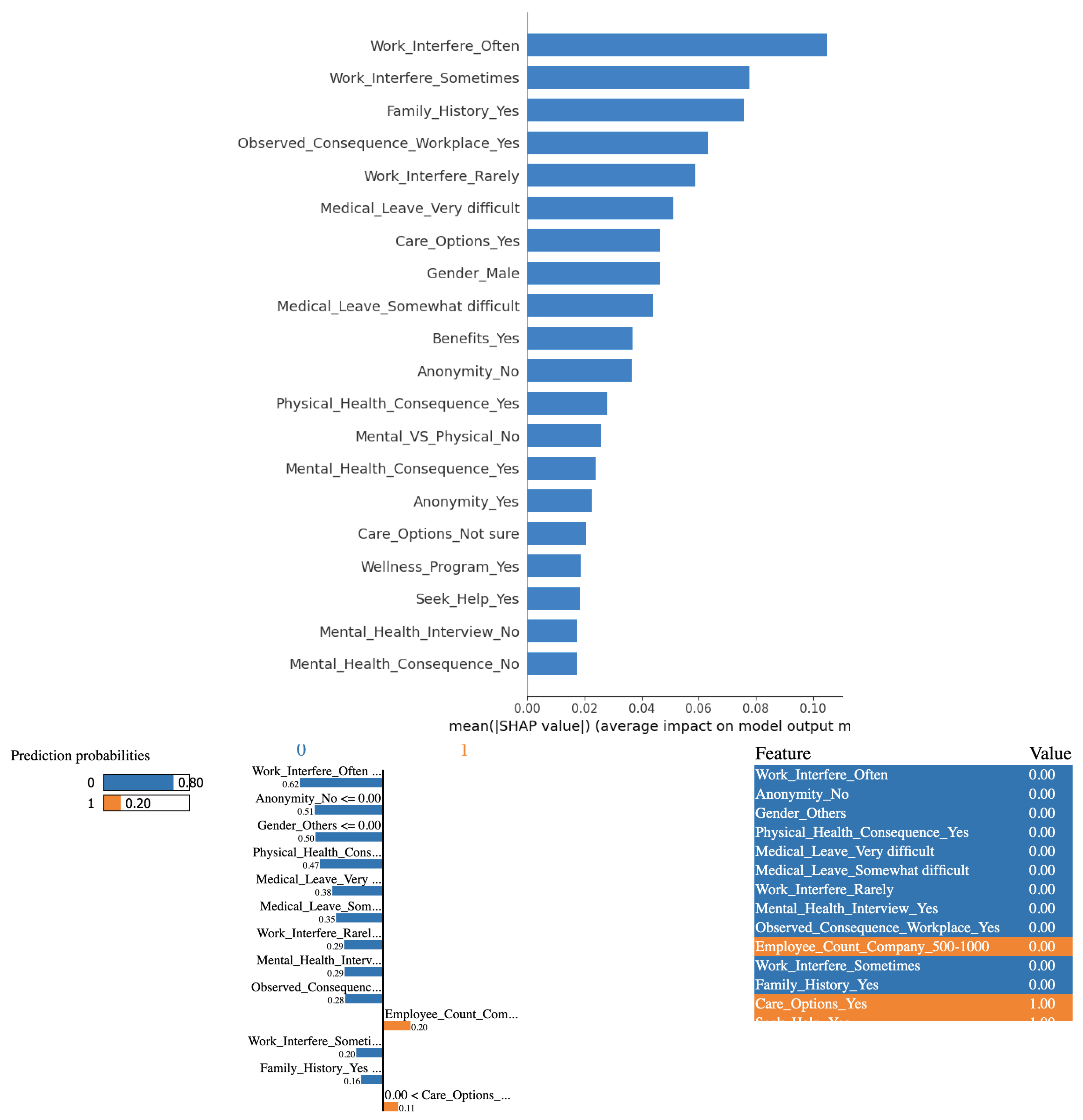
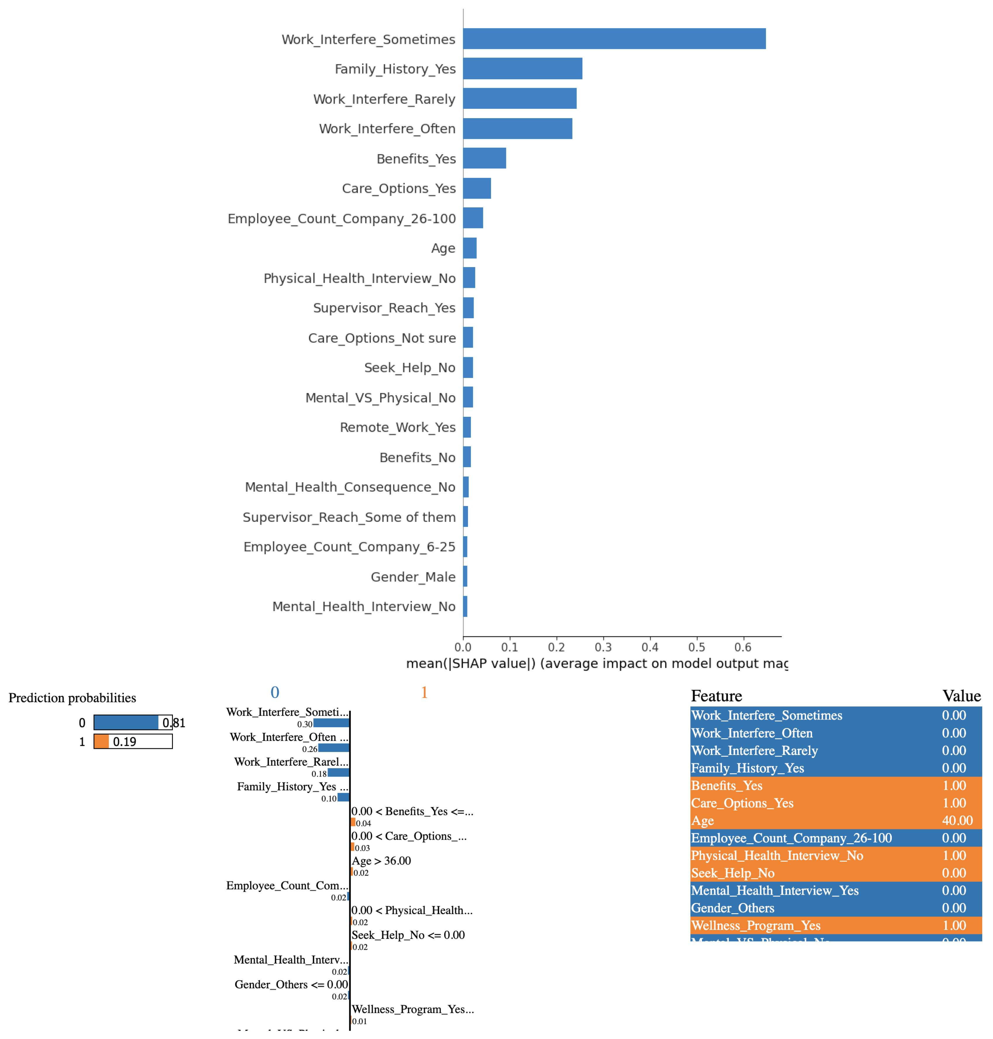
The analysis shows that K-NN differs significantly from logistic regression in terms of the explainability of their outcomes. Based on the results derived from employing the K-NN algorithm in conjunction with the SHAP and LIME methods, it is evident that the variables "Age" and "Work Interference(Sometimes)" significantly influence the determination of mental health conditions among study participants. The SHAP plot at the top in
Figure 4 is considerably different from the one for logistic regression in terms of the relative importance attached to the features. Like with logistic regression, answering "sometimes" to the survey question, "If you have a mental health condition, do you feel that it interferes with your work?" weighs far more to the logistic regression model in predicting than answering "often" or "rarely," which is counter-intuitive. But the SHAP values are more sensible than before because demographics like age, gender, and family history are given more weightage.
The results from LIME are also more sensible because for the specific instance at the bottom in
Figure 4, the person is predicted to have a mental health issue based on age among other factors, while answering no to the survey question, "If you have a mental health condition, do you feel that it interferes with your work?" and not having a family history pulled the outcome the other way (blue). It is also intuitive that the employer providing mental health benefits and the employee knowing about the care options that the employer provides contributed to the prediction of a mental health issue. However, the better sensibility of the explanations does not correlate with the not-so-appreciable evaluation metrics.
3.3. Explanations based on the Decision Tree Algorithm
Decision tree model performance is much better than that of K-NN. The evaluation metrics, Precision, Recall, F1 score, and Accuracy obtained from the application of the Decision Tree algorithm are tabulated in
Table 1.
3.3.1. SHAP and LIME analysis of the Decision Tree model performance
Decision trees are inherently interpretable. Here too, based on the outcomes derived from employing the Decision Tree algorithm in conjunction with the SHAP and LIME methods, it is evident that the variable "Work Interference(Sometimes)" significantly influences the determination of mental health conditions among study participants. This can be verified from
Figure 3. Like before, "Work Interference(Sometimes)" ranks higher than "Work Interference(often)" and "Work Interference(rarely)." The ranking for the other features is more sensible than that for logistic regression. The instance examined by LIME is predicted to not have any mental health issues based on the "no" to family history and work interference, which is a reasonable conclusion.
3.4. Explanations based on the Random Forest Algorithm
The random forest model performs reasonably well on the dataset. The evaluation metrics, Precision, Recall, F1 score, and Accuracy obtained from the application of Random Forest algorithm are tabulated in
Table 1.
3.4.1. SHAP and LIME analysis of the Random Forest model performance
As can be seen from
Figure 6, based on the outcomes derived from employing Random Forest algorithm in conjunction with the SHAP and LIME methods, the explanations are not entirely consistent with those from the decision tree model but similar.
3.5. Explanations based on the Gradient Boosting Algorithm
The evaluation metrics, Precision, Recall, F1 score, and Accuracy obtained from the application of the Gradient Boosting algorithm are tabulated in
Table 1. The model performs well on the dataset.
3.5.1. SHAP and LIME analysis of the Gradient Boosting model performance
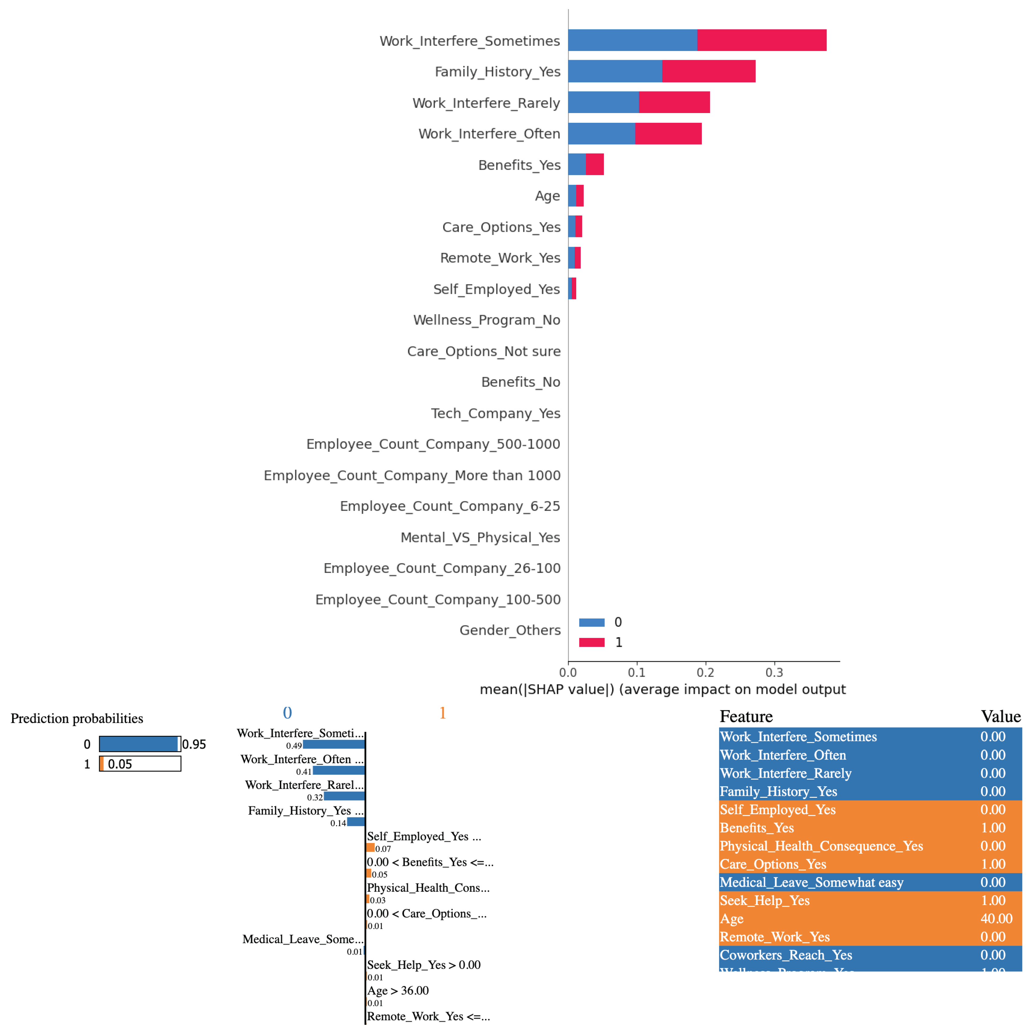
Like for other models, based on the outcomes derived from employing Gradient Boosting algorithm in conjunction with the SHAP and LIME methods, it is evident that the variable "Work Interference(Sometimes)" significantly influences the determination of mental health conditions among study participants. As can be seen from
Figure 7 there is nothing significantly different for this model.
3.6. Explanations based on the AdaBoost Algorithm
The evaluation metrics, Precision, Recall, F1 score, and Accuracy obtained from the application of the AdaBoost algorithm are tabulated in
Table 1. The metrics are similar to those for most of the other models.
3.6.1. SHAP and LIME analysis of the AdaBoost model performance
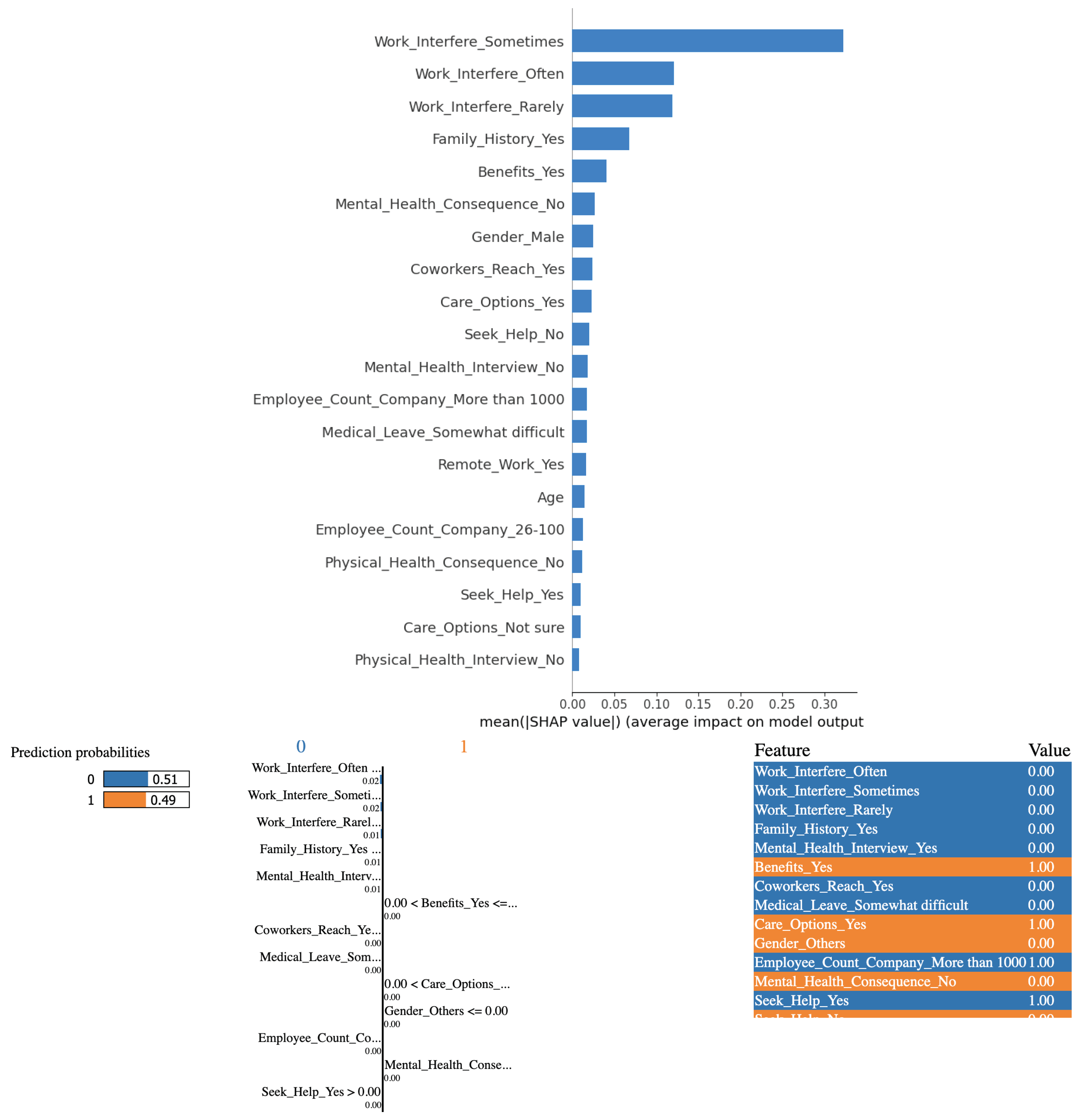
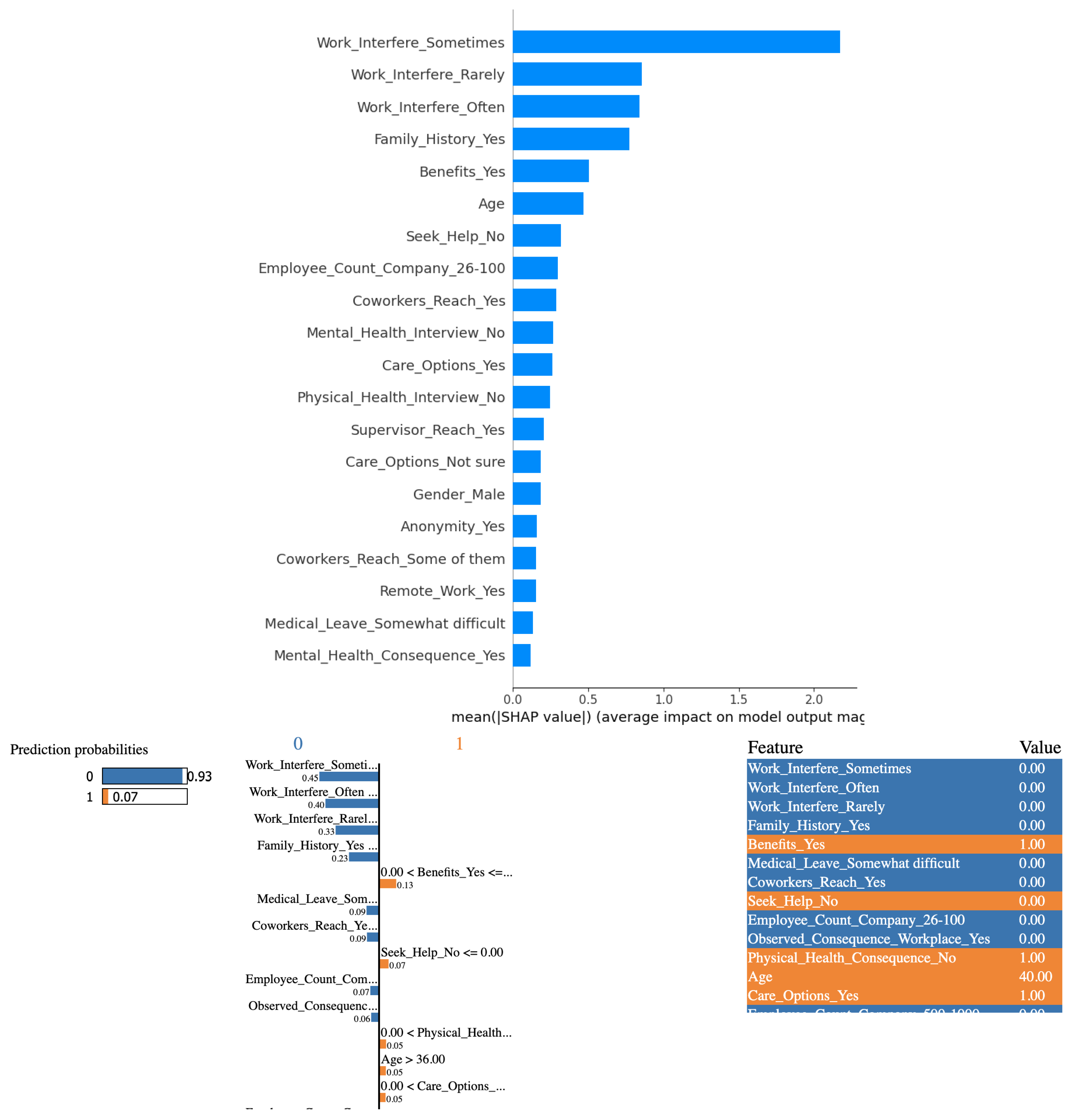
Based on the outcomes derived from employing the AdaBoost algorithm in conjunction with the SHAP and LIME methods, it is evident that the variables "Work Interference(Sometimes)" and "Work Interference(Often)" significantly influence the determination of mental health conditions among study participants. Interestingly, from
Figure 8, in the case chosen for analysis using LIME, none of the factors play a significant role in predicting a "no." The model is almost equanimous for this instance of data.
3.7. Explanations based on the Stochastic Gradient Descent Classifier Algorithm
The evaluation metrics, Precision, Recall, F1 score, and Accuracy obtained from the application of SGD Classifier algorithm are tabulated in
Table 1. The numbers are lower than those for the other algorithms.
3.7.1. SHAP and LIME analysis of the SGD Classifier model performance
From
Figure 9, based on the outcomes derived from employing Stochastic Gradient Descent algorithm in conjunction with the SHAP and LIME methods, it is evident that the variables "Work Interference(Sometimes)" and "Work Interference(Often)" significantly influence the determination of mental health conditions among study participants. But as pointed out earlier, the instance picked for analysis using LIME shows an erroneous outcome. SGD Classifier predicts a person not to have a mental health condition even when they answered "sometimes" to the survey question, "If you have a mental health condition, do you feel that it interferes with your work?" In doing so, the model relies more on the fact that the person did not answer with a "often" or "rarely" to the same question than on the fact that the person did answer "sometimes." The prediction is therefore highly misleading
3.8. Explanations based on the Naive Bayes Algorithm
The evaluation metrics, Precision, Recall, F1 score, and Accuracy obtained from the application of the Naive Bayes algorithm are tabulated in
Table 1. In terms of the metrics, the algorithm does not perform as well as Decision Tree or logistic regression.
3.8.1. SHAP and LIME analysis of the Naive Bayes model performance
As can be seen from
Figure 10, SHAP values are more logical than for other models. Based on the outcomes derived from employing Naive Bayes algorithm in conjunction with the SHAP and LIME methods, it is evident that the variable "Work Interference(Often)" significantly influences the determination of mental health conditions among study participants. LIME analysis is also more reasonable than for other models.
3.9. Explanations based on the Support Vector Machine Algorithm
The evaluation metrics, Precision, Recall, F1 score, and Accuracy obtained from the application of SVM algorithm are tabulated in
Table 1. The performance of the model in terms of these metrics is on par with other superlative models.
3.9.1. SHAP and LIME analysis of the SVM model performance
From
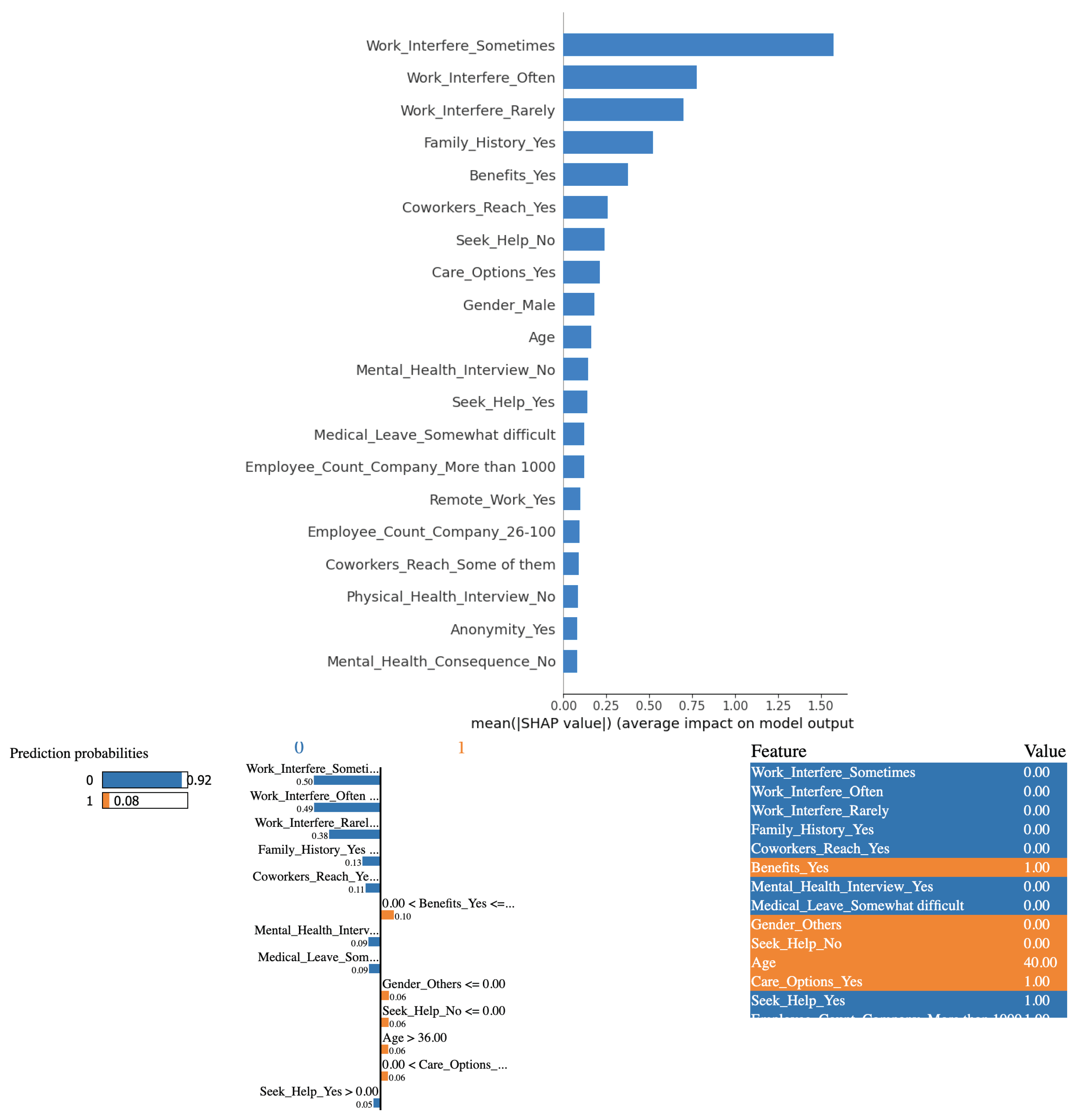
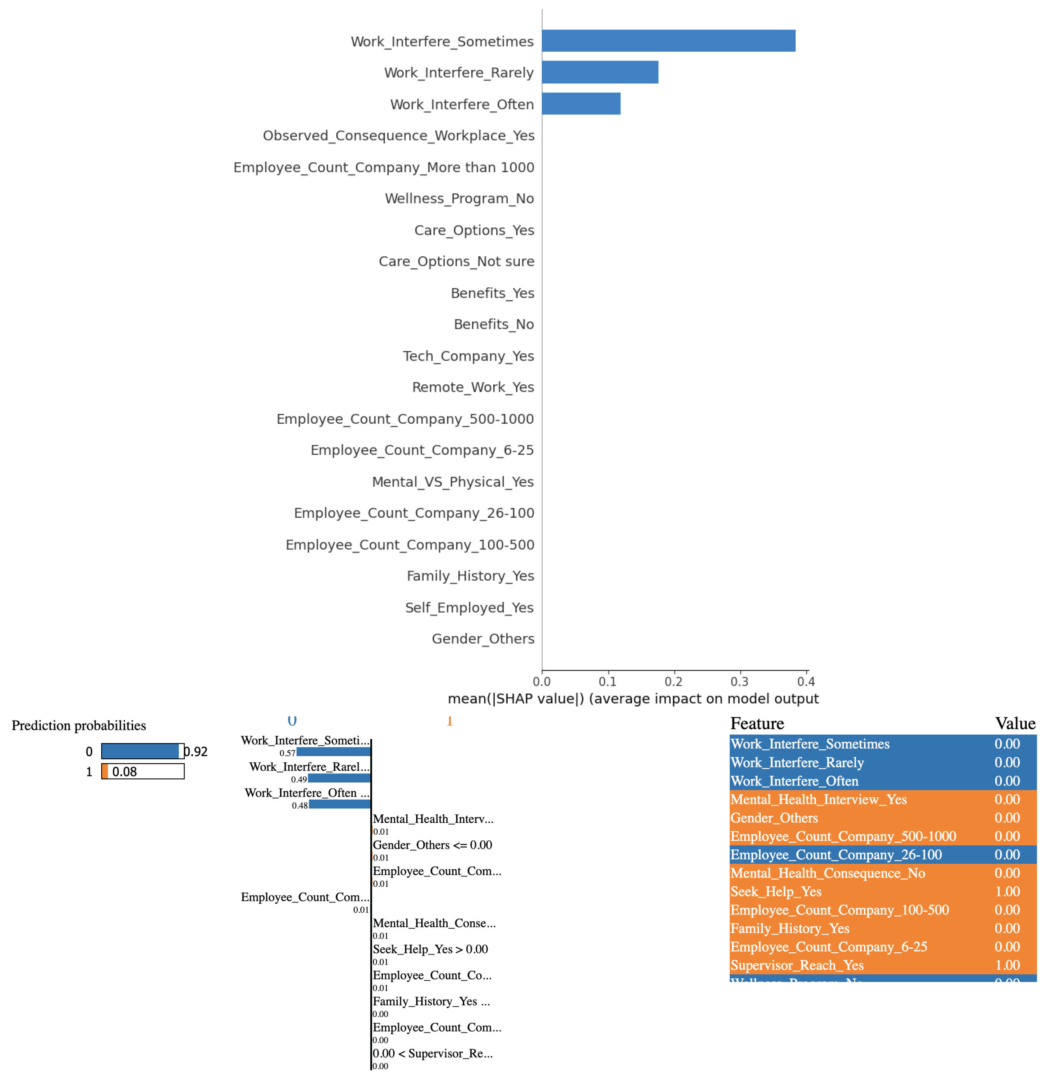
Figure 11, based on the outcomes derived from employing Support Vector Machine algorithm in conjunction with the SHAP and LIME methods, it is evident that the variable "Work Interference(Sometimes)" significantly influences the determination of mental health conditions among study participants. However, strangely, none of the answers to the other questions matter much to the model in making predictions. This holds consistently for both SHAP and LIME, locally and globally.
3.10. Explanations based on the XGBoost Algorithm
The evaluation metrics, Precision, Recall, F1 score, and Accuracy obtained from the application of XGBoost algorithm are tabulated in
Table 1. The algorithm performs reasonably well in terms of these metrics.
3.10.1. SHAP and LIME analysis of the XGBoost model performance
From
Figure 12, based on the outcomes derived from employing XGBoost algorithm in conjunction with the SHAP and LIME methods, it is evident that the variable "Work Interference(Sometimes)" significantly influences the determination of mental health conditions among study participants. The findings are not too different from those for most other models.
3.11. Explanations based on the LightGBM Algorithm
The evaluation metrics, Precision, Recall, F1 score, and Accuracy obtained from the application of LightGBM algorithm are tabulated in
Table 1. The numbers are similar to other best-performing models.
3.11.1. SHAP and LIME analysis of the LightGBM model performance
As can be seen from
Figure 13, based on the outcomes derived from employing Light GBM algorithm in conjunction with the SHAP and LIME methods, it is evident that the variable "Work Interference(Sometimes)" significantly influences the determination of mental health conditions among study participants. Here too, there are no major surprises.
4. Discussion
The experiments show that the models behave differently than what is commonly expected. Given that the survey is for understanding mental health issue prevalence in the tech sector, the factors that are supposed to impact the prediction the most should relate to the tech sector. In fact, the literature confirms a correlation between mental health prognosis and the environment in the tech sector. Using the same dataset, researchers [
34] state, "When comparing those who work in tech to those who do not work in tech, there was a clear majority of those who do work in tech." It can therefore be expected that answers to questions such as "Is your employer primarily a tech company/organization?" should have ranked higher in the model’s predictions. However, the factors that came up at the top did not have to do anything specific to the tech sector. In fact, for some of the models like Support Vector Machine and Decision Tree, tech sector related features do not matter at all.
Machine learning models are not expected to imply causality. Though the organization, OSMI, which does the survey year after year targets workers in the tech sector, it is clear from the results that indeed, there is no causality established. Despite the high accuracy of the models in predicting mental health, they do not in any way imply that working in the tech industry is a cause for mental health issues. The explainability techniques used for this work too, do not indicate any causality. It is therefore important to understand the limitations and potential pitfalls of relying solely on machine learning models for drawing major conclusions based on an intuitive interpretation of the results.
Literature [
35] also claims the effectiveness of machine learning algorithms in predicting mental health outcomes. Our experiments demonstrate that although the evaluation metrics for the models are superlative, the justification of the outcomes from these models is not intuitive or reasonable. It is also apparent that models differ in their explainability. Accordingly, the research questions are answered as follows.
-
RQ1: How reliable are the evaluation metrics such as accuracy in assessing the machine learning model performance in making important predictions?
The experiments demonstrate that the evaluation metrics fall short in their trustworthiness. The metrics are high even when the models relied on an unsound ranking of the features.
-
RQ2: How well do the explainable AI techniques, SHAP and LIME complement the conventional evaluation metrics?
The attribution techniques, SHAP and LIME can add corroboratory evidence of the model’s performance. The results from the experiment show the complementary nature of the plots from the explainability methods and the evaluation metrics. LIME is substantially impacted by the choice of hyperparameters and may not fully comply with some legal requirements [
36]. However, for the experiments described in this paper, the profile of LIME explanations was mostly consistent with the explanations from SHAP. A summary metric for the explainability aspects may further enhance the utility of the methods.
-
RQ3: How do the various machine learning algorithms compare when it comes to the explainability of their outcomes?
The majority of the machine learning algorithms behave quite similarly with respect to the explainability of the outcomes. However, some algorithms like SGD Classifier perform poorly in terms of the explainability of their outcomes, while Naive Bayes performs slightly better.
It is quite evident from the experiments that focusing only on achieving high performance metrics from machine learning models, particularly used for critical applications like mental health prediction, can be misleading and ethically concerning. The work emphasizes the crucial role of explainability techniques in providing insights into how models arrive at their predictions, fostering trust and transparency. The results also underscore the broader applicability of XAI across various domains of application of machine learning. A promising direction for research is in developing metrics and more frameworks that evaluate models not just on accuracy based performance but also on their interpretability and trustworthiness.
5. Conclusions
Machine learning is increasingly being applied to critical predictions such as mental health. The literature contains several tall claims about the effectiveness of the various machine learning algorithms in predicting mental health outcomes. Multiple of those papers use the same dataset as used in this work. The experiments described in this paper show that the claims need to be corroborated using results from the explainability techniques to gain insights into the models’ working and justification of the outcomes. The findings can be easily generalized to other domains and datasets as there is nothing specific in the dataset or experiments detailed in this paper nor are there any assumptions that limit the generalizability. The work proves that merely achieving superlative evaluation metrics can be dangerously misleading and may infringe upon ethical horizons. A future direction is to investigate methods to quantify the effectiveness of machine learning models in terms of the insights from their explainability.
Author Contributions
Conceptualization, V.P.; methodology, V.P.; software, H.K.; validation, H.K. and V.P.; formal analysis, V.P.; investigation, V.P. and H.K.; resources, H.K.; writing—original draft preparation, V.P.; writing—review and editing, V.P.; visualization, H.K.; supervision, V.P.; project administration, V.P.; All authors have read and agreed to the published version of the manuscript.
Funding
This research received no external funding.
Institutional Review Board Statement
Not applicable—no animal or human data collection as part of this project.
Informed Consent Statement
Not applicable.
Data Availability Statement
No new data were created or analyzed in this study. Data sharing is not applicable to this article.
Conflicts of Interest
The authors declare no conflict of interest.
References
- Illness, O.S.M. OSMI Mental Health in Tech Survey, 2014.
- Ribeiro, M.T.; Singh, S.; Guestrin, C. Interpretable Machine Learning: A Unified Approach based on Proximity Measures. International Conference on Machine Learning, 2016, pp. 997–1005.
- Lundberg, S.M.; Lee, S.I.; Erion, A.; Johnson, M.J.; Vennekamp, P.; Bengio, Y. A Unified Approach to Interpretable Explanatory Modeling. International Conference on Machine Learning, 2020, pp. 4769–4777.
- Sujal, B.; Neelima, K.; Deepanjali, C.; Bhuvanashree, P.; Duraipandian, K.; Rajan, S.; Sathiyanarayanan, M. Mental health analysis of employees using machine learning techniques. 2022 14th International Conference on COMmunication Systems & NETworkS (COMSNETS). IEEE, 2022, pp. 1–6. [CrossRef]
- Mitravinda, K.; Nair, D.S.; Srinivasa, G. Mental Health in Tech: Analysis of Workplace Risk Factors and Impact of COVID-19. SN computer science 2023, 4, 197. [Google Scholar] [CrossRef] [PubMed]
- Li, Y. Application of Machine Learning to Predict Mental Health Disorders and Interpret Feature Importance. 2023 3rd International Symposium on Computer Technology and Information Science (ISCTIS). IEEE, 2023, pp. 257–261. [CrossRef]
- Vorbeck, J.; Gomez, C. Algorithms and Anxiety: An Investigation of Mental Health in Tech. MA Data Analytics & Applied Social Research 2022. [Google Scholar]
- Baptista, M.L.; Goebel, K.; Henriques, E.M. Relation between prognostics predictor evaluation metrics and local interpretability SHAP values. Artificial Intelligence 2022, 306, 103667. [Google Scholar] [CrossRef]
- Ratul, Q.E.A.; Serra, E.; Cuzzocrea, A. Evaluating attribution methods in machine learning interpretability. 2021 IEEE International Conference on Big Data (Big Data). IEEE, 2021, pp. 5239–5245. [CrossRef]
- Hu, B.; Tunison, P.; Vasu, B.; Menon, N.; Collins, R.; Hoogs, A. XAITK: The explainable AI toolkit. Applied AI Letters 2021, 2, e40. [Google Scholar] [CrossRef]
- Ueda, D.; Kakinuma, T.; Fujita, S.; Kamagata, K.; Fushimi, Y.; Ito, R.; Matsui, Y.; Nozaki, T.; Nakaura, T.; Fujima, N.; others. Fairness of artificial intelligence in healthcare: review and recommendations. Japanese Journal of Radiology 2024, 42, 3–15. [Google Scholar] [CrossRef] [PubMed]
- Kerz, E.; Zanwar, S.; Qiao, Y.; Wiechmann, D. Toward explainable AI (XAI) for mental health detection based on language behavior. Frontiers in psychiatry 2023, 14. [Google Scholar] [CrossRef] [PubMed]
- Band, S.S.; Yarahmadi, A.; Hsu, C.C.; Biyari, M.; Sookhak, M.; Ameri, R.; Dehzangi, I.; Chronopoulos, A.T.; Liang, H.W. Application of explainable artificial intelligence in medical health: A systematic review of interpretability methods. Informatics in Medicine Unlocked, 2023; 101286. [Google Scholar] [CrossRef]
- Srinivasu, P.N.; Sirisha, U.; Sandeep, K.; Praveen, S.P.; Maguluri, L.P.; Bikku, T. An Interpretable Approach with Explainable AI for Heart Stroke Prediction. Diagnostics 2024, 14, 128. [Google Scholar] [CrossRef] [PubMed]
- Rahmatinejad, Z.; Dehghani, T.; Hoseini, B.; Rahmatinejad, F.; Lotfata, A.; Reihani, H.; Eslami, S. A comparative study of explainable ensemble learning and logistic regression for predicting in-hospital mortality in the emergency department. Scientific Reports 2024, 14, 3406. [Google Scholar] [CrossRef] [PubMed]
- Pendyala, V.S.; Kim, H. Analyzing and Addressing Data-driven Fairness Issues in Machine Learning Models used for Societal Problems. 2023 International Conference on Computer, Electrical & Communication Engineering (ICCECE). IEEE, 2023, pp. 1–7. [CrossRef]
- Arslan, Y.; Lebichot, B.; Allix, K.; Veiber, L.; Lefebvre, C.; Boytsov, A.; Goujon, A.; Bissyandé, T.F.; Klein, J. Towards refined classifications driven by shap explanations. International Cross-Domain Conference for Machine Learning and Knowledge Extraction. Springer, 2022, pp. 68–81.
- Slack, D.; Hilgard, S.; Jia, E.; Singh, S.; Lakkaraju, H. Fooling lime and shap: Adversarial attacks on post hoc explanation methods. Proceedings of the AAAI/ACM Conference on AI, Ethics, and Society, 2020, pp. 180–186.
- Hassija, V.; Chamola, V.; Mahapatra, A.; Singal, A.; Goel, D.; Huang, K.; Scardapane, S.; Spinelli, I.; Mahmud, M.; Hussain, A. Interpreting black-box models: a review on explainable artificial intelligence. Cognitive Computation 2024, 16, 45–74. [Google Scholar] [CrossRef]
- Viswan, V.; Shaffi, N.; Mahmud, M.; Subramanian, K.; Hajamohideen, F. Explainable artificial intelligence in Alzheimer’s disease classification: A systematic review. Cognitive Computation 2024, 16, 1–44. [Google Scholar] [CrossRef]
- Longo, L.; Brcic, M.; Cabitza, F.; Choi, J.; Confalonieri, R.; Del Ser, J.; Guidotti, R.; Hayashi, Y.; Herrera, F.; Holzinger, A. ; others. Explainable artificial intelligence (XAI) 2.0: A manifesto of open challenges and interdisciplinary research directions. Information Fusion, 2024; 102301. [Google Scholar] [CrossRef]
- Cox, D.R. The regression analysis of binary sequences. Journal of the Royal Statistical Society: Series B (Methodological) 1958, 20, 215–232. [Google Scholar] [CrossRef]
- Cover, T.M. Patterns in random sequences. IEEE Transactions on Information Theory 1967, 13, 1–14. [Google Scholar]
- Quinlan, J.R. A decision tree method for the identification of antibacterial active compounds. International Conference on Machine Learning, 1986, pp. 248–257.
- Breiman, L. Random forests. Machine learning 2001, 45, 5–32. [Google Scholar] [CrossRef]
- Friedman, J.H. Greedy function approximation: A general boosting framework. Annals of statistics 2002, 38, 1183–1232. [Google Scholar]
- Freund, Y.; Schapire, R.E. A decision-theoretic generalization of on-line learning and an application to boosting. Journal of computer and system sciences 1997, 55, 119–139. [Google Scholar] [CrossRef]
- LeCun, Yann A., e.a. Stochastic gradient descent training for large-scale online linear classification. Advances in neural information processing systems, 2015, pp. 248–256.
- Russell, S.W. The Bayesian approach to automatic speech recognition. IEEE Transactions on Speech and Audio Processing 1995, 16, 227–252. [Google Scholar]
- Cortes, C.; Vapnik, V. Support-vector networks. Machine learning 1995, 20, 273–297. [Google Scholar] [CrossRef]
- Chen, Tianqi, e.a. XGboost: A scalable system for state-of-the-art gradient boosting 2016. pp. 785–794.
- Ke, Guolin, e.a. Lightgbm: A highly efficient gradient boosting decision tree. Advances in Neural Information Processing Systems, 2017, pp. 3146–3154.
- Shapley, L.S. ; others. A value for n-person games 1953. [CrossRef]
- Uddin, M.M.; Farjana, A.; Mamun, M.; Mamun, M. Mental health analysis in tech workplace. Proceedings of the 7th North American International Conference on Industrial Engineering and Operations Management, 2022, pp. 12–14.
- Bajaj, V.; Bathija, R.; Megnani, C.; Sawara, J.; Ansari, N. Non-Invasive Mental Health Prediction using Machine Learning: An Exploration of Algorithms and Accuracy. 2023 7th International Conference on Intelligent Computing and Control Systems (ICICCS). IEEE, 2023, pp. 313–321.
- Molnar, C. Interpretable machine learning; Lulu. com, 2020.
Figure 1.
Flowchart illustrating the methodology
Figure 1.
Flowchart illustrating the methodology
Figure 2.
Bar graph comparing the results from various machine learning algorithms
Figure 2.
Bar graph comparing the results from various machine learning algorithms
Figure 3.
Insights into what drives the logistic regression predictions, to understand how and why the predictions were made. (Top) Visualization of how features nudge the Logistic Regression predictions up or down using SHAP values. (Bottom) Interpretable Explanations using LIME’s localized approach. LIME uses weighted tweaks to features, revealing their impact on predictions.
Figure 4.
(Top) SHAP bar chart showing overall feature importance when K-NN model is used. Features with larger absolute SHAP values (both positive and negative) have a stronger influence on the prediction (Bottom) Interpretable Explanations of the K-NN model using LIME’s localized approach
Figure 4.
(Top) SHAP bar chart showing overall feature importance when K-NN model is used. Features with larger absolute SHAP values (both positive and negative) have a stronger influence on the prediction (Bottom) Interpretable Explanations of the K-NN model using LIME’s localized approach
Figure 5.
(Top) Quantifying feature influence on decision tree like a game of fair contributions using SHAP (Bottom) Understanding why decision tree makes a specific prediction using LIME’s localized approach.
Figure 5.
(Top) Quantifying feature influence on decision tree like a game of fair contributions using SHAP (Bottom) Understanding why decision tree makes a specific prediction using LIME’s localized approach.
Figure 6.
(Top) SHAP bar chart showing overall feature importance when random forest model is used. Features with larger absolute SHAP values (both positive and negative) have a stronger influence on the prediction (Bottom) Interpretable Explanations of the random forest model using LIME’s localized approach
Figure 7.
(Top) SHAP bar chart showing overall feature importance when the Gradient Boosting model is used. (Bottom) Interpretable Explanations of the Gradient Boosting model predictions using LIME’s localized approach
Figure 7.
(Top) SHAP bar chart showing overall feature importance when the Gradient Boosting model is used. (Bottom) Interpretable Explanations of the Gradient Boosting model predictions using LIME’s localized approach
Figure 8.
(Top) SHAP values chart when AdaBoost algorithm is used.(Bottom) LIME’s localized approach shows that the AdaBoost algorithm is almost equanimous in predicting for this instance
Figure 8.
(Top) SHAP values chart when AdaBoost algorithm is used.(Bottom) LIME’s localized approach shows that the AdaBoost algorithm is almost equanimous in predicting for this instance
Figure 9.
(Top) SHAP and (Bottom) LIME plots for SGD Classifier outcomes
Figure 9.
(Top) SHAP and (Bottom) LIME plots for SGD Classifier outcomes
Figure 10.
(Top) SHAP bar chart showing overall feature importance when Naive Bayes algorithm is used. (Bottom) Interpretable Explanations of the Naive Bayes algorithm using LIME’s localized approach
Figure 10.
(Top) SHAP bar chart showing overall feature importance when Naive Bayes algorithm is used. (Bottom) Interpretable Explanations of the Naive Bayes algorithm using LIME’s localized approach
Figure 11.
(Top) SHAP bar chart showing overall feature importance when SVM model is used. (Bottom) Interpretable Explanations of the SVM model using LIME’s localized approach
Figure 11.
(Top) SHAP bar chart showing overall feature importance when SVM model is used. (Bottom) Interpretable Explanations of the SVM model using LIME’s localized approach
Figure 12.
(Top) SHAP and (Bottom) LIME plots for XGBoost outcomes
Figure 12.
(Top) SHAP and (Bottom) LIME plots for XGBoost outcomes
Figure 13.
(Top) SHAP and (Bottom) LIME plots for Light GBM algorithm outcomes
Figure 13.
(Top) SHAP and (Bottom) LIME plots for Light GBM algorithm outcomes
Table 1.
Summary of results from applying various machine learning on the dataset
Table 1.
Summary of results from applying various machine learning on the dataset
| Evaluation Metrics |
|---|
| Models |
Precision |
Recall |
F1 score |
Accuracy |
| LR |
0.8279 |
0.8944 |
0.8599 |
0.8456 |
| KNN |
0.7428 |
0.5226 |
0.6135 |
0.6534 |
| DT |
0.7949 |
0.9547 |
0.8675 |
0.8465 |
| RF |
0.7857 |
0.8844 |
0.8321 |
0.8121 |
| GB |
0.8364 |
0.8994 |
0.8668 |
0.8544 |
| AdaBoost |
0.9206 |
0.2914 |
0.4427 |
0.6137 |
| SGD |
0.9206 |
0.2914 |
0.4427 |
0.6137 |
| NB |
0.7483 |
0.5678 |
0.6457 |
0.6719 |
| SVM |
0.7949 |
0.9547 |
0.8675 |
0.8465 |
| XGB |
0.8146 |
0.8391 |
0.8267 |
0.8148 |
| LGBM |
0.8240 |
0.8944 |
0.8578 |
0.8439 |
Table 2.
Summary of finetuned hyperparameters for each model used Grid Search
Table 2.
Summary of finetuned hyperparameters for each model used Grid Search
| Model |
Hyper Parameters |
| LR |
max iter : 1000 |
| KNN |
n neighbors: 5 |
| DT |
criterion: "gini", max depth: 4 |
| RF |
n estimators : 200, max depth: 12, min samples leaf: 6, min samples split: 20 |
| GB |
n estimators: 50, learning rate: 1.0, max depth: 1 |
| AdaBoost |
n estimators: 50 |
| SGD |
max iter: 1000, loss: ’log loss’, tol: 1e−3
|
| NB |
None |
| SVM |
kernel: "linear", probability: True |
| XGB |
None |
| LGBM |
num round = 10 |
|
Disclaimer/Publisher’s Note: The statements, opinions and data contained in all publications are solely those of the individual author(s) and contributor(s) and not of MDPI and/or the editor(s). MDPI and/or the editor(s) disclaim responsibility for any injury to people or property resulting from any ideas, methods, instructions or products referred to in the content. |
© 2024 by the authors. Licensee MDPI, Basel, Switzerland. This article is an open access article distributed under the terms and conditions of the Creative Commons Attribution (CC BY) license (http://creativecommons.org/licenses/by/4.0/).
