1. Introduction
Count data analysis is a statistical approach used to analyze data that consists of non-negative integer values, representing the number of occurrences of a specific event within a given context. This data type is commonly encountered in various fields, such as biology, economics, social sciences, and engineering. However, count data poses unique challenges due to its discrete nature, often exhibiting characteristics such as excessive zeros and overdispersion [
11].
Excessive zeros refer to an unusually high number of observations with a count of zero, which cannot be adequately explained by standard statistical models. It requires specialized techniques to be appropriately accounted for in the analysis to avoid biased model estimates [
27,
31]. Overdispersion occurs when the variance of the count data is higher than expected, indicating that additional sources of variation need to be accounted for beyond what the basic models can handle [
20].
To address these complexities and effectively model count-based phenomena, specialized statistical models known as count models have been developed. Two commonly used count models are Poisson regression and Negative Binomial regression. Poisson regression is suitable for count data with low variability, assuming that the mean and variance of the data are equal. However, in cases where overdispersion is present, Poisson regression may not provide accurate results. Negative Binomial regression, on the other hand, allows for overdispersion and provides a more flexible approach to model count [
25].
In this article, we aim to provide a comprehensive overview of count data analysis and count models. We explore the concept of zero inflation and its impact on count models, demonstrating how it can lead to model misspecification if not properly addressed. In addition, we introduce two statistical tests: Likelihood Ratio Tests (LRT) and the Vuong Test [
8]. LRT is used to compare nested models and assess the improvement in model fit when additional parameters are added. On the other hand, the Vuong Test is a model selection criterion that compares non-nested models, making it ideal for comparing count models with and without zero inflation.
Furthermore, the article emphasizes the practicality of our approach by providing the complete code we created that implements the Vuong Test in the widely used Python programming language. Python is renowned for its ease of use and extensive libraries, making it an excellent choice for data analysts and researchers [
44]. By creating a Python implementation of the Vuong Test, we enhance the accessibility and applicability of this essential model selection technique in real-world scenarios, enabling readers to make informed model selection decisions and perform robust analysis of count-based phenomena in their projects.
2. Count data
Count data refers to the observations made about events or items that are enumerated. More specifically, in the context of statistics, count data refers to the number of occurrences of an event within a fixed period. It only contains positive integer values that go from zero to some greater value, because an event cannot occur a negative number of times [
11,
12]. Examples of count data include the number of speeding tickets received in a year, the number of crimes on campus per semester, or the number of trips per year a person makes.
Following the concept of count data, it’s possible to define count variable as a list or array of count data [
11]. Count variables indicate how many times something has happened, and can be used as response variables in statistical modeling when the goal is to understand or predict the factors influencing the count [
10].
3. Count models
In simple terms, a statistical model helps us understand how different variables are related to each other. It provides a mathematical representation of how one variable or a set of variables can explain or predict another variable. Specifically, when we have a count variable, the statistical model helps us explain the counts using one or more explanatory variables [
11,
18].
Statistical models are considered stochastic because they are based on probability functions. This means that they take into account the uncertainty and variability inherent in real-world data. Instead of providing exact predictions or explanations, the model provides a probabilistic framework that describes the likelihood or probability of different outcomes [
13]. By utilizing statistical models, we can analyze and quantify the relationships between variables, make predictions, and assess the statistical significance of explanatory factors. These models allow us to gain insights into the underlying patterns and processes driving the count variable, accounting for the inherent randomness and variability observed in real-world phenomena. In the scope of count data, those statistical models have applications that exploit the full probability distribution of counts to provide comprehensive predictions. This capability enhances our ability to interpret and utilize count data effectively in various applications, such as forecasting, risk assessment, resource allocation, and decision-making [
18].
When using count variables in Ordinary Least Squares (OLS) regression, there are potential issues to consider. OLS regression, which has minimal assumptions about predictors, allows count variables to be used as predictors with one caveat. If the count variable has very little variability, which can happen with count data having a small range, the regression coefficient associated with that predictor becomes unstable and has a large standard error [
9]. It’s important to note that this instability is not unique to count predictors - any predictor with low variability would result in an unstable regression coefficient.
However, different problems arise when a count variable is used as the outcome or dependent variable in OLS regression. When the average count value of the outcome variable is relatively high, OLS regression can generally be applied without significant difficulty. But when the mean of the outcome variable is low, OLS regression produces undesirable outcomes, including biased standard errors and significance tests [
12].
So, while count variables can be used as predictors in OLS regression with caution, using count variables as outcome variables in OLS regression can result in inefficient, inconsistent, and biased estimates. Even though there are situations in which the Linear Regression Model (LRM) provides reasonable results, it is much safer to employ regression models specifically designed for count outcomes, as they offer improved statistical power and appropriately handle the specific characteristics of count data [
10,
12]. Examples of such models include Poisson Regression, Negative Binomial Regression (NB), and variations of these models for zero-inflated counts (ZIP and ZINB). These models consider the discrete nature of count variables, their variability, and the specific statistical assumptions needed for accurate estimation and inference [
10,
20].
Generalized linear models offer a versatile method for addressing a wide variety of response modeling issues. The most frequently used responses are Normal, Poisson, and Binomial, but other distributions may also be employed [
22,
23]. When dealing with count data, we typically begin by estimating the parameters using a Poisson regression model because of its simplicity. In this scenario, the dependent variable in a Poisson regression model should adhere to a Poisson distribution with the mean equaling the variance [
24]. However, this property is frequently violated in empirical research, as it is common for there to be overdispersion, where the variance of the dependent variable exceeds its mean. In such instances, we will estimate a negative binomial regression model [
26].
4. Poisson and Negative Binomial Models
The Poisson distribution is distinct from the normal distribution in several ways that make it more appealing for representing the characteristics of count data. Firstly, the Poisson distribution is a discrete distribution that only assumes probability values for non-negative integers. This feature of the Poisson distribution makes it an ideal choice for modeling count outcomes, which can only take on integer values of 0 or more [
12]. The Poisson distribution, for a given observation i, has the following probability of occurrence of a count m (m = 0, 1, 2...) in a given exposure:
In (
1),
is the expected number of occurrences or the estimated incidence rate ratio of the phenomenon under study for a given exposure. In the Poisson distribution, the mean and variance of the variable under study must be equal to
. This characteristic is known as the equidispersion of the Poisson distribution. If this condition is satisfied, a Poisson regression model can be calculated, which is described as follows:
In (
2),
stands for the constant,
(j = 1, 2, …, k) are the calculated parameters for each explanatory variable,
are the explanatory variables (either metrics or dummies) and the subscript i denotes each observation in the sample (i = 1, 2, …, n, where n is the size of the sample).
The log-likelihood function, which must be maximized, can be written as:
As previously noted, the data is assumed to have equidispersion. If this is not the case, a negative binomial regression model could be used for estimation [
11]. The NB distribution uses an additional parameter to model overdispersion. In other words, an NB-distributed random variable is equivalent to a Poisson random variable with a random, gamma-distributed mean, allowing it to model unobserved individual heterogeneity [
27].
For a given observation
i (i = 1, 2, … , n, where n is the sample size), the probability distribution function of the variable
will be given by the following:
In (
4),
is called the shape parameter (
),
is called the rate parameter (
) and, for
and integer,
can be approximated by
. The log-likelihood function for the NB2 regression, which must be maximized, can be written as:
For a more detailed discussion of both the Poisson and NB distributions, see [
20,
25,
29].
5. Zero-inflated count data models
Simply testing for overdispersion and using a NB model may not be enough. It’s important to note that overdispersion can be caused by an excess of zeros in the data, and this zero inflation may need to be accounted for in the model [
27,
31].
When data is zero-inflated, it is necessary to modify the Poisson or NB procedure to prevent incorrect estimation of model parameters and standard errors, as well as incorrect specification of the distribution of test statistics. Ignoring these misspecifications can lead to incorrect conclusions about the data and introduce uncertainty into research and practice. As a result, the use of zero-inflated Poisson (ZIP) and zero-inflated negative binomial (ZINB) models has grown in popularity across a wide range of fields [
21].
According to [
32], zero-inflated regression models are considered a combination of a count data model and a binary data model. They are used to investigate the reasons for a certain number of occurrences (counts) of a phenomenon, as well as the reasons for the occurrence (or not) of the phenomenon itself, regardless of the number of counts observed.
Facing this scenario, according to [
30], the first step is to address potential overdispersion in the distribution by comparing Poisson versus NB models, using statistical tests such as the likelihood ratio test (LRT) and the Wald test. The next step is to assess whether the distribution has an excess of zeros by comparing Poisson versus ZIP or NB versus ZINB models, using the Vuong test [
8]. If the zero-inflated version of the model fits the data significantly better than the standard model, it is considered evidence that the data contains an excess of zeros [
27].
5.1. Zero Inflated Poisson Models
In the ZIP model, the probability
p of observing zero counts for a given observation
i (
, where n is the sample size), or
, is determined by combining a dichotomous component with a count component. As a result, the probability
of observing zero counts due solely to the dichotomous component must be established. The probability of observing a specific count
m (
), or
, is determined by the probability expression of the Poisson distribution, multiplied by (
) [
25]. To sum up, for
, we have the following equations, on which
(
).
It is evident that if
, the probability distribution in expression
6 simplifies to the Poisson distribution, even for instances where
. In other words, ZIP regression models have two processes that generate zeros. One is due to the binary distribution, which generates what are known as structural zeros. The other is due to the Poisson distribution, which generates count data, including what is known as sample zeros [
25].
The log-likelihood function of a ZIP regression model (
7) should also be maximized.
5.2. Zero Inflated Negative Binomial Models
In the ZINB models, The probability of no counts for a given observation i, or
, is also calculated by adding a dichotomous component to a count component. The chance of a specific count m (
), or
, now follows the probability expression of the Poisson-Gamma distribution [
25]. In equation (
8), for
,
(
),
represents the inverse of the shape parameter of a given Gamma distribution.
The log-likelihood function of a ZINB regression model (
9) should also be maximized.
6. Likelihood Ratio Tests for Model Selection: Vuong Test
The decision to use either conventional count regression or zero-inflated modeling is based on the balance between avoiding overfitting and accurately representing the empirical features of the data. One way to determine if a zero-inflated model is necessary is to compare its fit to that of a standard count model. This test is important because choosing the wrong model can have consequences. If the standard model is chosen when the zero-inflated model is more appropriate, an important part of the data-generating process may be overlooked. On the other hand, if the zero-inflated model is chosen when it’s not necessary, the model becomes unnecessarily complicated by adding an extra equation [
33].
With this dilemma in mind, researchers commonly use the Vuong test [
8] to determine whether the zero-inflated model fits the data statistically significantly better than count regression with a single equation. The Vuong test is a method for comparing the fit of two models to the same data using maximum likelihood. Its purpose is to test the null hypothesis that the two models fit the data equally well. The models being compared need not be nested, and one of them doesn’t need to be the correct specification [
33].
7. Vuong Test Implementation on Python
Python is currently experiencing a surge in popularity as a programming language, and this can be attributed to several factors. Firstly, Python is known for its ease of use and accessibility, making it an attractive option for beginners. Additionally, the learning curve for Python is relatively fast, allowing new users to quickly become proficient. Another major draw for Python is the vast array of high-quality packages available for data science and machine learning applications.
A few libraries in Python already support statistical and econometric analysis, such as statsmodels [
39] and pandas [
40]. However, when it comes to general statistics, Python lags behind the R programming language. As a result, many scientists continue to rely on R for their statistical analysis [
38].
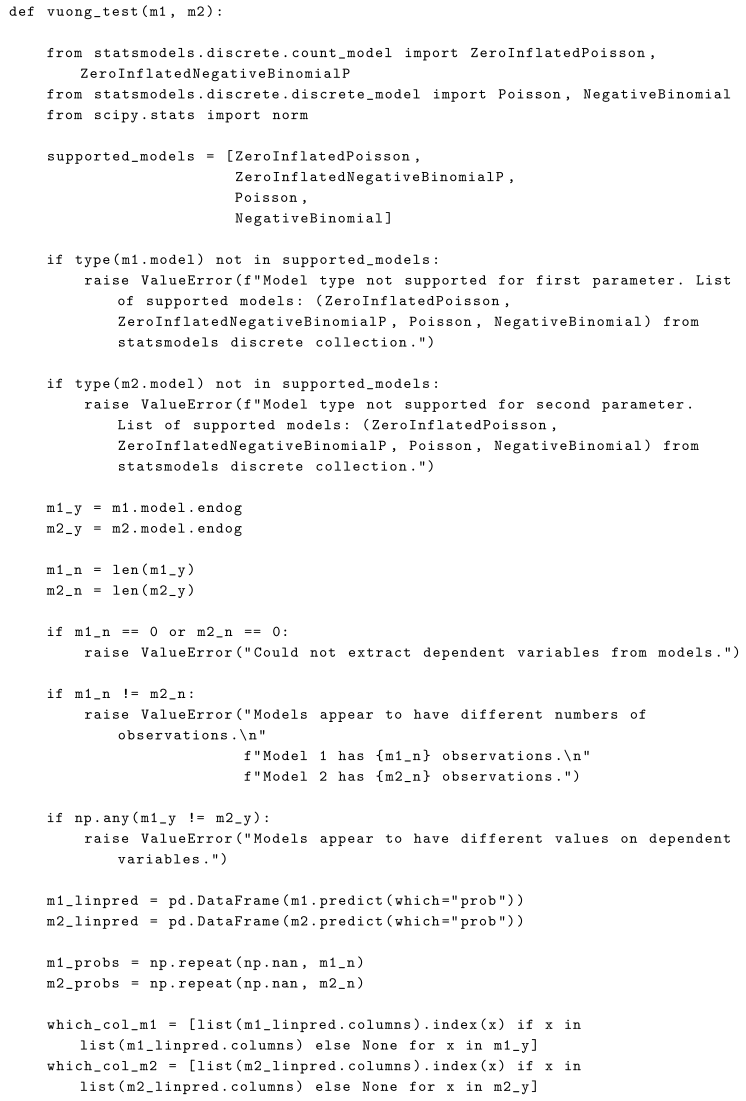
In an effort to make Python more complete for statistical analysis, a gap was identified in the Vuong test, which currently lacks an implementation in Python. So, we present a code that implements the Vuong test in Python. In addition, we demonstrate its use on a database [
41]. Other machine learning and deep learning studies have already been covered in this same journal, such as [
45,
46,
47].
7.1. Corruption Database
According to [
41], in a empirical approach developed for evaluating the role of both social norms and legal enforcement in corruption by studying parking violations among United Nations diplomats living in New York City, diplomatic immunity is a privilege that allows mission personnel and their families to avoid paying parking fines. This was the case until November 2002. Illegally parking can be considered an act of corruption, as it is an abuse of power for personal gain. Comparing parking violations by diplomats from different societies can serve as a measure of the extent of corruption norms or culture.
The data set contains the following information:
Country name
Code of the country
Number of parking violations
Number of UN Mission Diplomats in 1998
Indicator (Yes/No) that the data is before or after the law enforcement
Corruption Index - CI [
42]
The data set is organized in a table as follows in
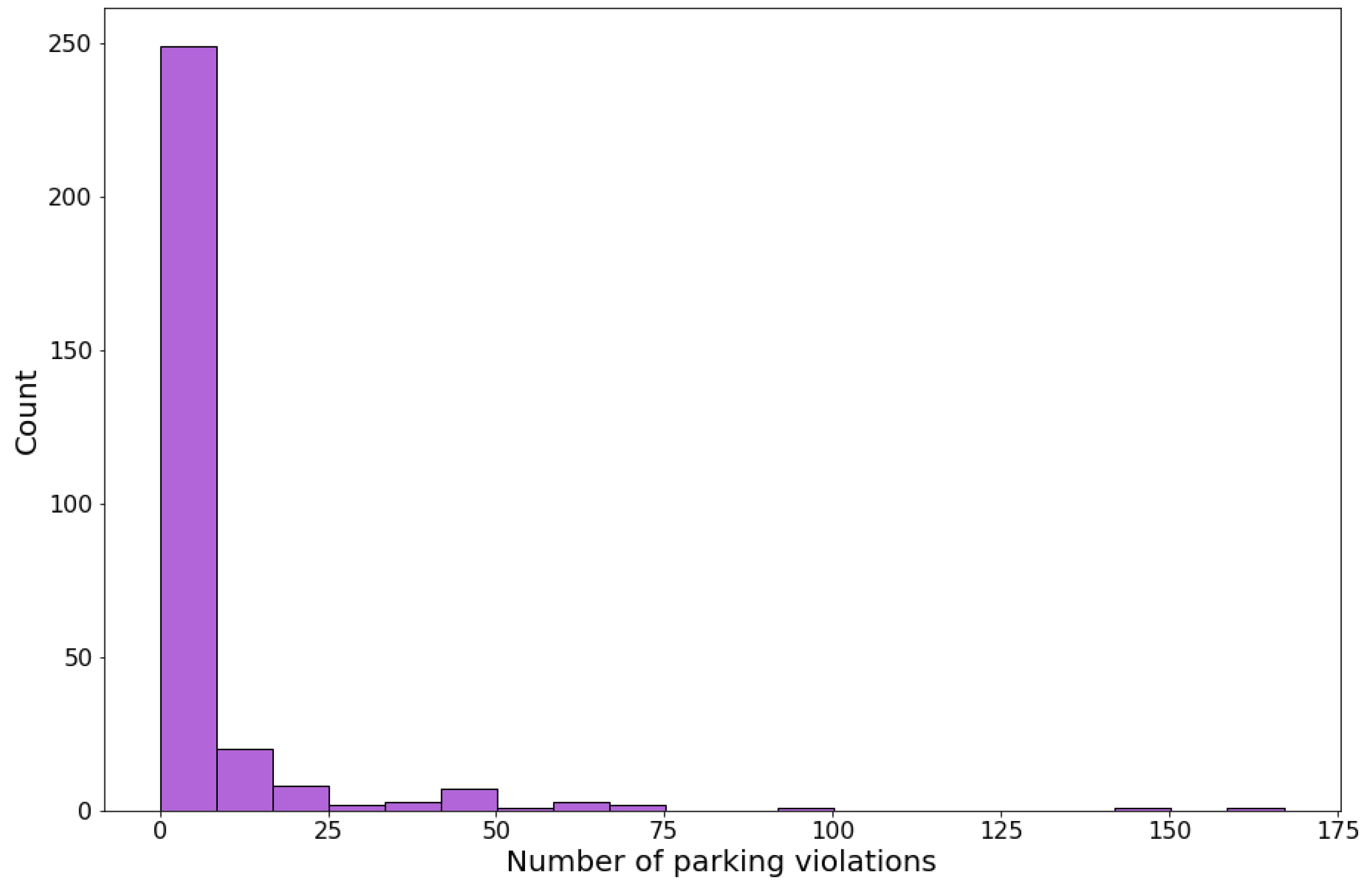
Table 1. It contains data from 149 countries, and it has 298 rows, given that which country has 2 rows (one for data before law enforcement and the other for after law enforcement). Also, the histogram of the data (counts per number of parking violations) is shown in
Figure 1.
7.2. Code Availability
The Python code that was developed to implement the Vuong test [
8] is available on the [sec:Appendix A]Appendix A - Code. It’s important to execute the following command before running the code to update the statsmodel version required.
7.3. Computational Environment and Analysis Setup
The analysis was conducted on a notebook equipped with an Intel Core i5-1235U processor (1.30 GHz, 12 cores, 12 threads), 20 GB of DDR4 RAM, and a Intel IRIS Xe graphics card. The computer ran Windows 11 as the operating system. Analysis was performed using Python 3.11.3 with libraries including NumPy 1.26.3, pandas 2.2.0, statsmodels 0.14.1 and scipy 1.12.0. No parallelization was utilized, as the algorithm ran efficiently on a single processor.
7.4. Efficiency and Performance of the Algorithm
The algorithm employed in this study is not computationally demanding, as evidenced by its smooth execution and negligible runtime. It ran effortlessly on the available hardware, completing its tasks in a remarkably short amount of time.
8. Results
Firstly, it was elaborated a preliminary diagnosis of equidispersion (observation of possible equality between the mean and the variance of the dependent variable ’violations’). As can be seen in
Table 2, the mean (
) and the variance (
) are very distant from each other. Therefore, there is a preliminary indication of overdispersion.
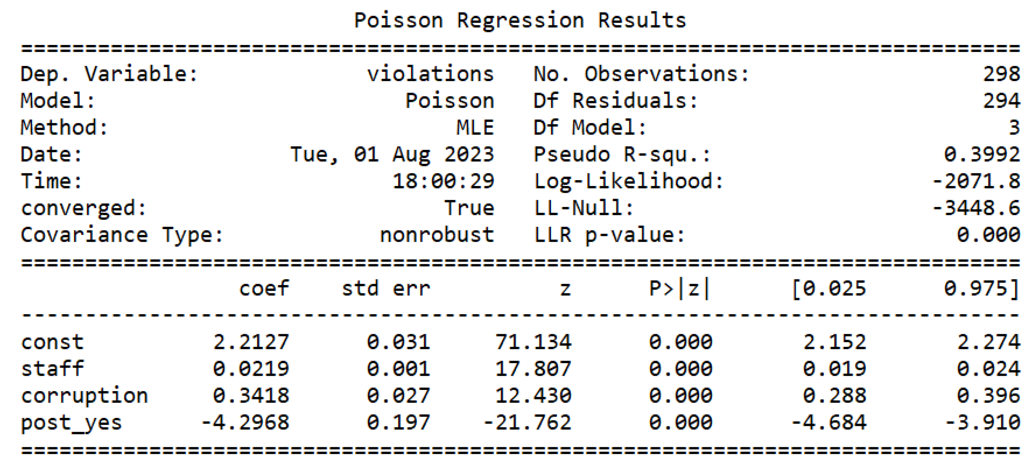
The next step was to estimate the Poisson model, as can be seen in
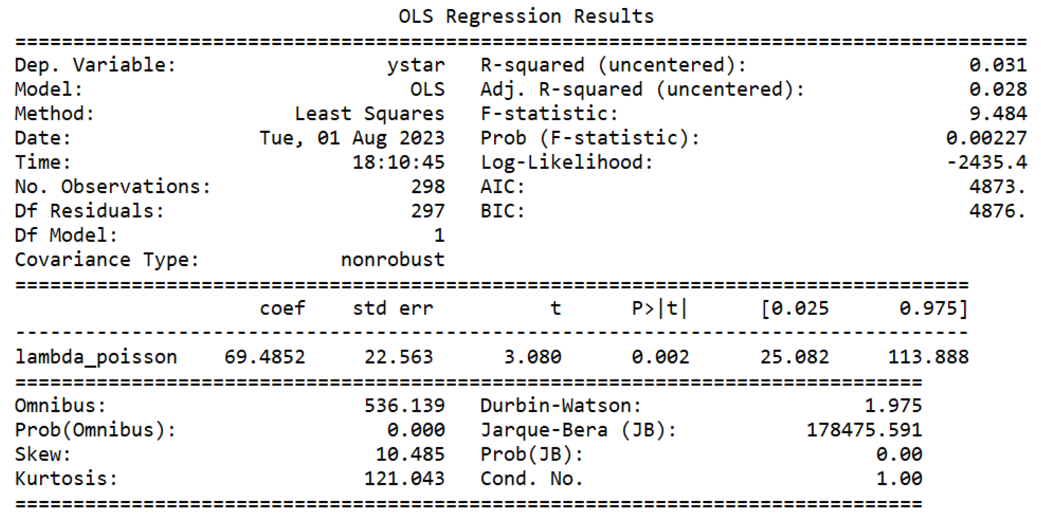
Figure 2. Then, it was tested if the data has equidispersion [
43]. The test can be seen in
Figure 3. As the p-value of the t-test corresponding to the
parameter of
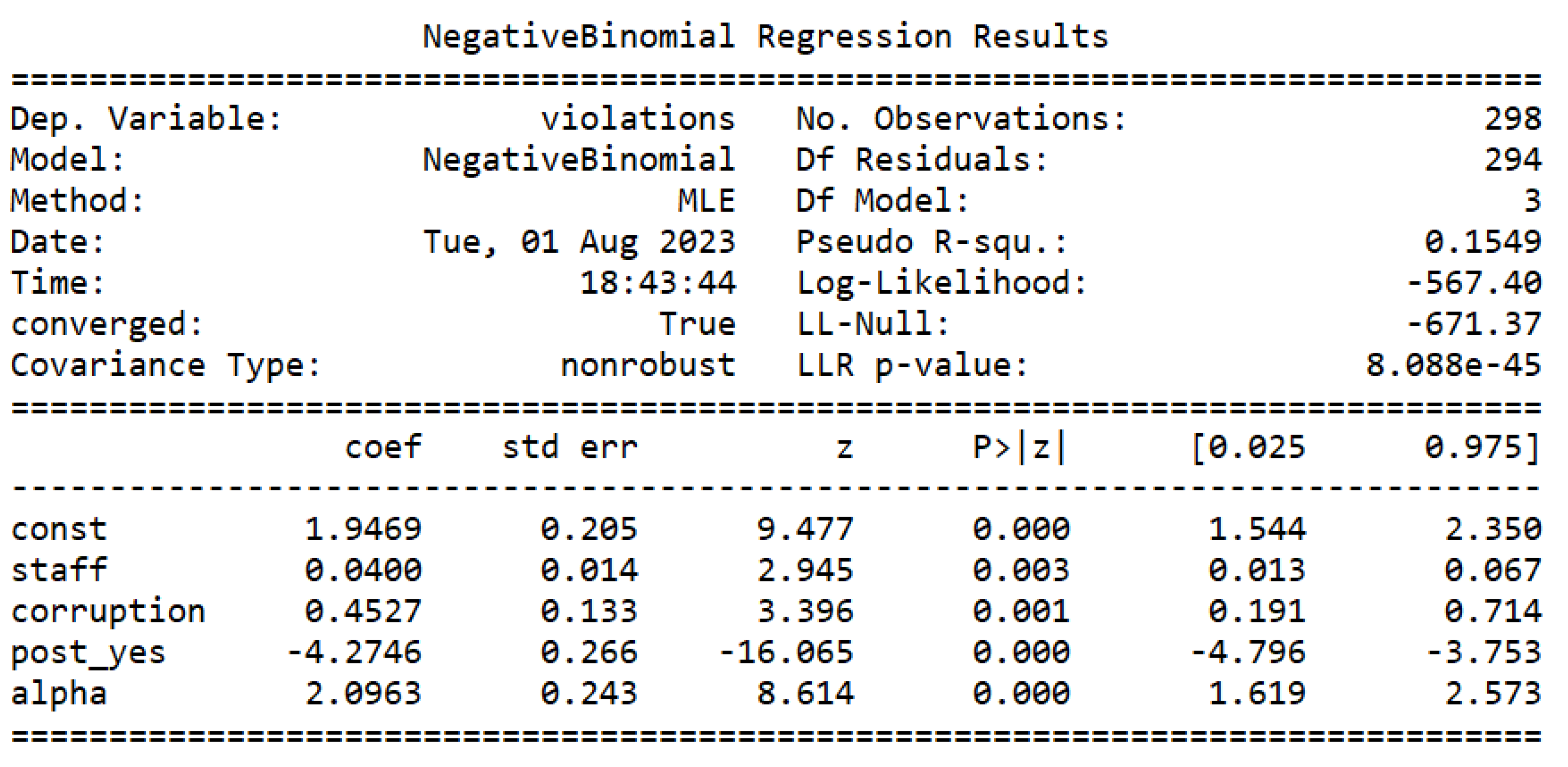
is less than 0.05, as it is worth 0.02, it can be stated that the data of the dependent variable present overdispersion, making the estimated Poisson regression model inadequate. Then, we proceed to estimate the negative binomial model, as can be seen in
Figure 4.
By comparing the Log-Likelihood (LL) of the Poisson and negative binomial models, as it is possible to see in
Figure 2 and
Figure 4, we can see that the NB has a smaller LL than Poisson. LL is close to
for the NB model, and close to
for the Poisson model.
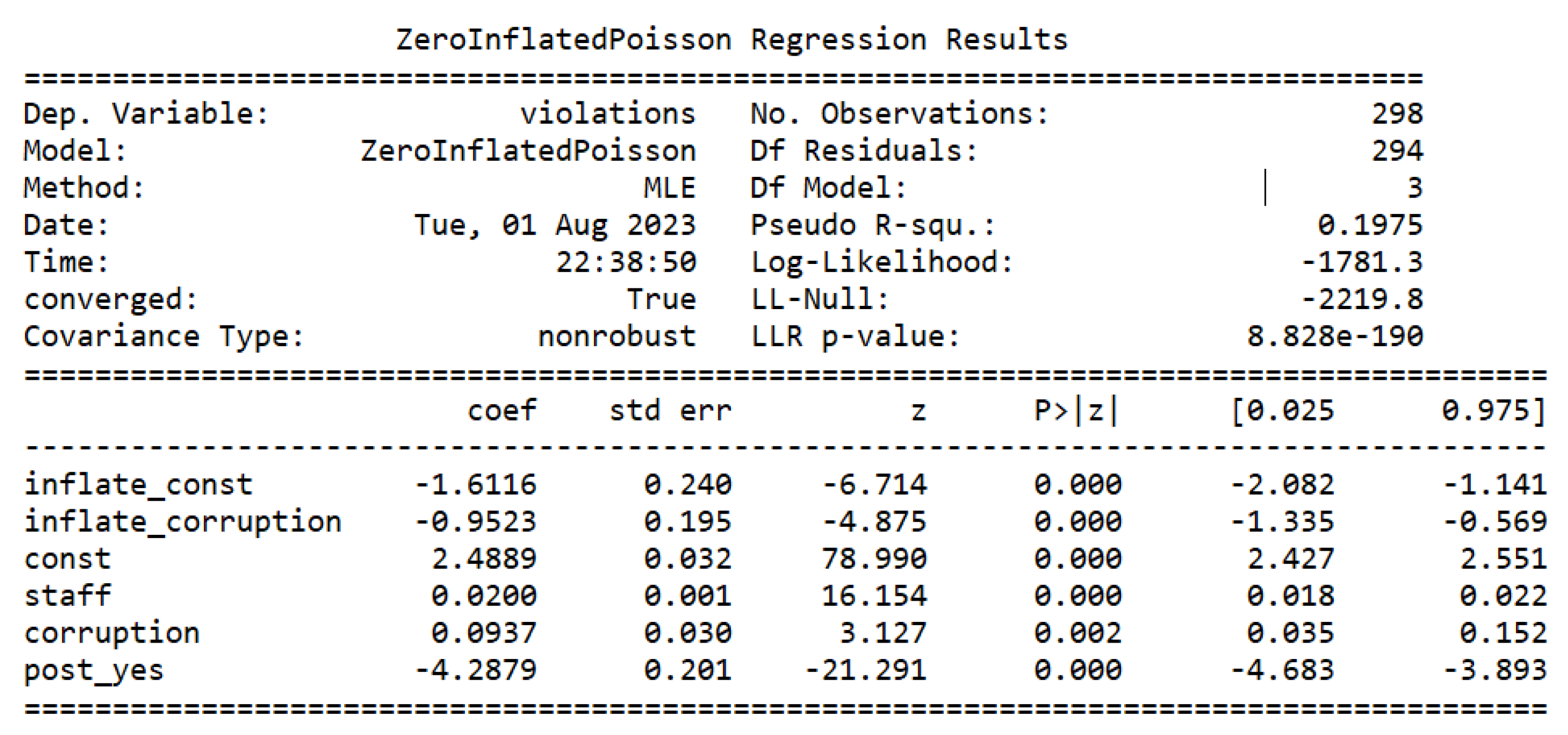
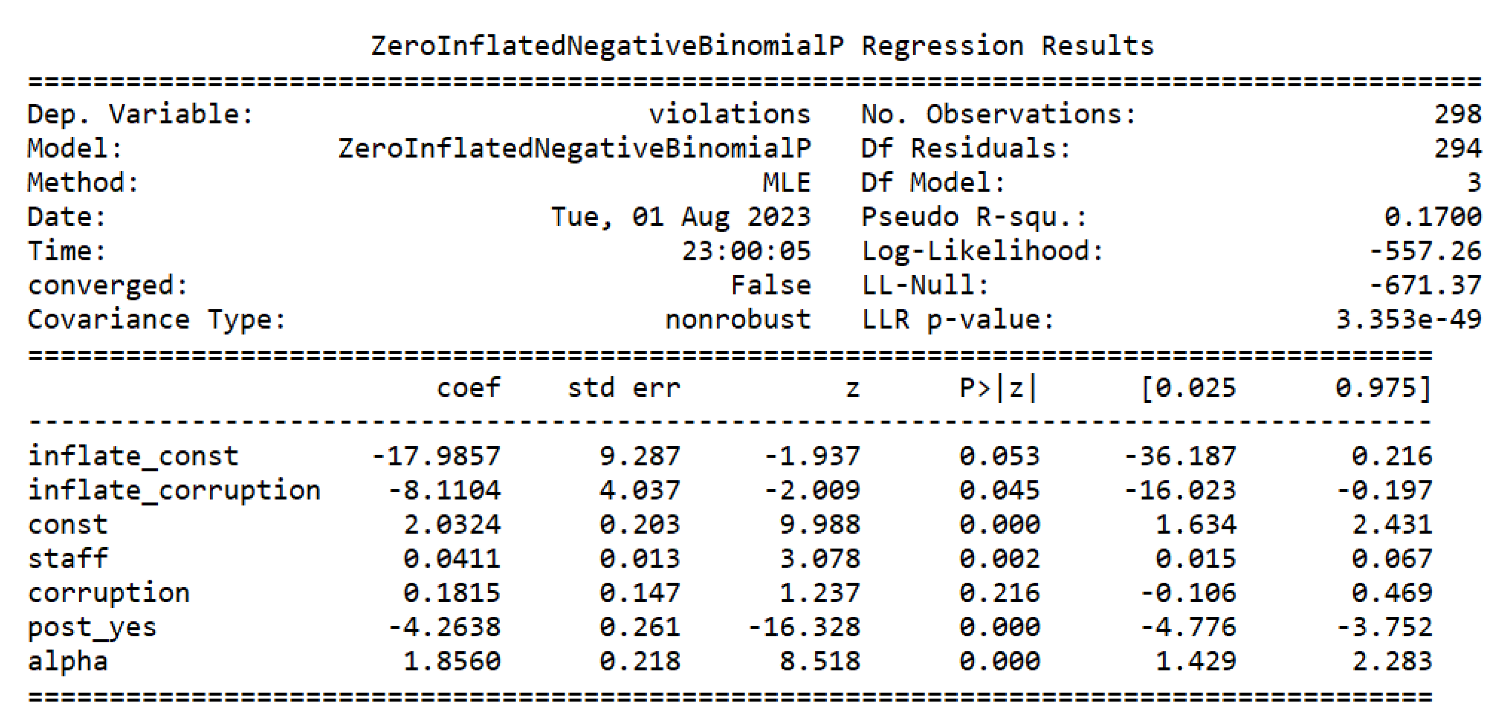
The next step is to estimate the zero-inflated Poisson model and the zero-inflated NB model, which can be seen in
Figure 5 and
Figure 6, respectively.
After that, it is possible to apply the Vuong test that was developed to compare the Poisson model (
Figure 2) with the ZIP model (
Figure 5) and to compare the NB model (
Figure 4) with the ZINB model (
Figure 6). The code returns the outputs on
Table 3.
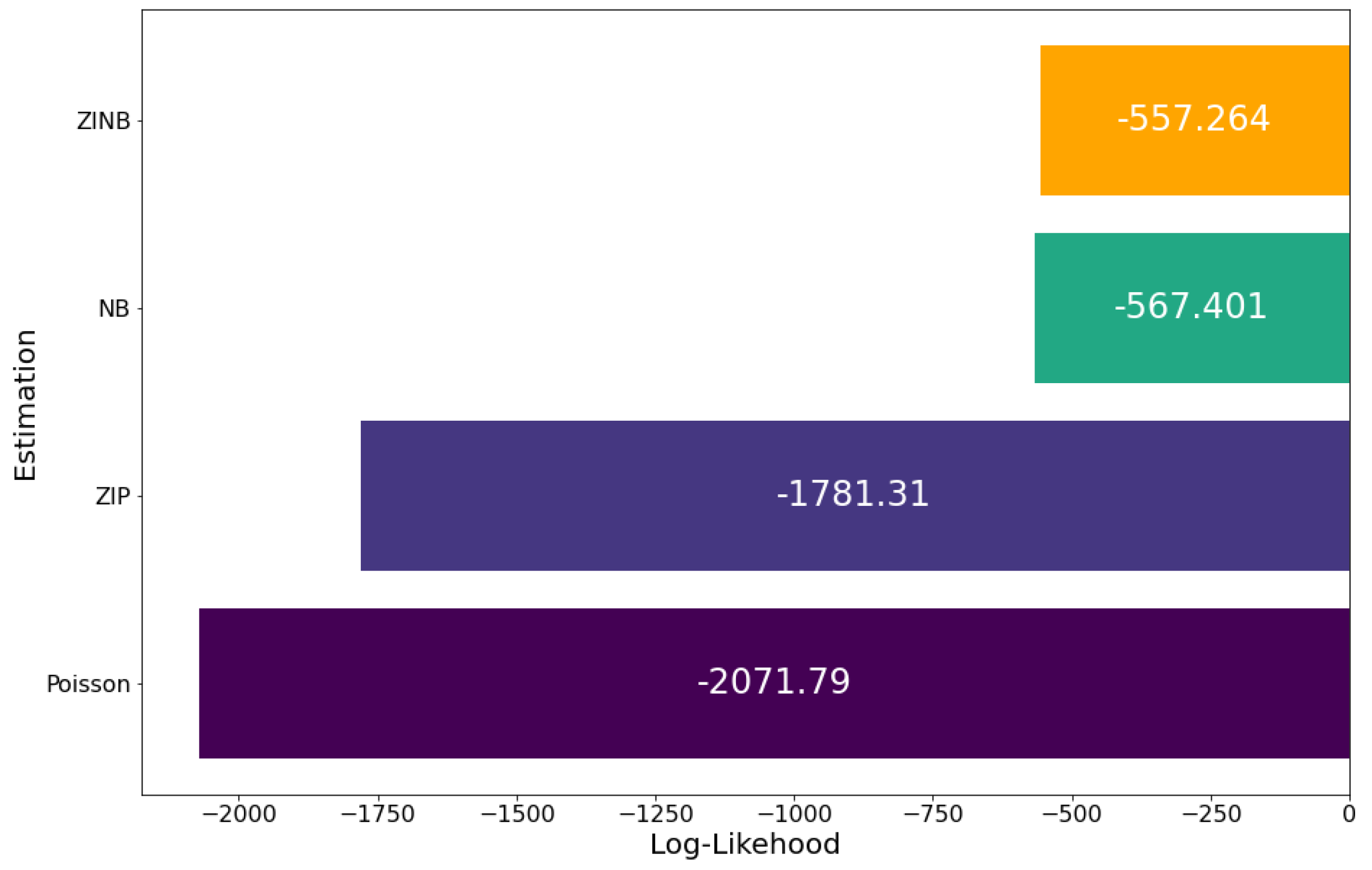
By comparing the Log-Likelihood (LL) of the ZIP and ZINB models, it is possible to see, on the
Figure 7, that the ZINB has a smaller LL than ZIP. LL is close to
for the ZINB model, and close to
for the ZIP model.
9. Discussion
In the Vuong test, positive and statistically significant values indicate the adequacy of the ZIP or ZINB model. Negative and statistically significant values indicate the adequacy of the traditional Poisson model or negative binomial model [
25].
As it was previously discussed, the data is overdispersed, making the estimated Poisson model inadequate. In this case, the Vuong test is used to choose between the NB model and the ZINB model. Considering that the Vuong test resulted in
, with a p-value
(
Table 3), the traditional NB model is a better option than the ZINB at a significance level of 95%.
In
Figure 8, there is a comparison of the models. It includes the observed, predicted, and fitted values and confidence intervals for Poisson, NB, ZIP, and ZINB.
10. Conclusion
In conclusion, the Vuong Test that we developed from scratch using the Python programming language has proven to be a useful tool for choosing between regular or zero-inflated models. Prior to our work, this test did not exist in the Python environment. Now, other researchers can benefit from our contribution by using the code we have made available in [sec:Appendix A]Appendix A of this paper to apply the Vuong Test in their research using Python.
Funding
This research received no external funding.
Data Availability Statement
Conflicts of Interest
The authors declare no conflicts of interest.
Abbreviations
The following abbreviations are used in this manuscript:
| ZIP |
Zero Inflated Poisson |
| ZINB |
Zero Inflated Negative Binomial |
| LRT |
Likelihood Ration Tests |
| OLS |
Ordinary Least Squares |
| NB |
Negative Binomial |
| LL |
Log-Likelihood |
| CI |
Confidence Interval |
Appendix A. Vuong Test code in Python
References
- Fahrmeir, L.; Kneib, T.; Lang, S.; Marx, B. Regression: Models, Methods and Applications; Springer-Verlag: New York, 2013. [Google Scholar]
- Lesaffre, E.; Komárek, A.; Jara, A. The Bayesian approach. In Statistical and Methodological Aspects of Oral Health Research; Lesaffre, E., Feine, J., Leroux, B., Declerck, D., Eds.; John Wiley and Sons: Chichester, 2009; pp. 315–338. [Google Scholar]
- Gómez, G.; Luz Calle, M.; Oller, R.; Langohr, K. Tutorial on methods for interval-censored data and their implementation in Statistical Modelling. 2009, 9, 259–297. [Google Scholar] [CrossRef]
- Kneib, T. Beyond mean regression. Statistical Modelling 2013, 13, 275–303. [Google Scholar] [CrossRef]
- Komárek, A.; Lesaffre, E. Bayesian semi-parametric accelerated failure time model for paired doubly-interval-censored data. Statistical Modelling 2006, 6, 3–22. [Google Scholar] [CrossRef]
- Li, L.; Simonoff, J. S.; Tsai, C.-L. Tobit model estimation and sliced inverse regression. Statistical Modelling 2007, 7, 107–123. [Google Scholar] [CrossRef]
- Waldmann, E.; Kneib, T.; Yue, Y. R.; Lang, S.; Flexeder, C. Bayesian semiparametric additive quantile regression. Statistical Modelling 2013, 13, 223–252. [Google Scholar] [CrossRef]
- Vuong, Q. H. Likelihood ratio tests for model selection and non-nested hypotheses. Econometrica: journal of the Econometric Society 1989, 307–333. [Google Scholar] [CrossRef]
- Cohen, J.; Cohen, P.; West, S. G.; Aiken, L. S. Applied multiple regression/correlation analysis for the behavioral sciences; Routledge, 2013. [Google Scholar]
- Long, J. Scott; Freese, Jeremy. Regression models for categorical dependent variables using Stata; Stata press, 2006; Volume 7. [Google Scholar]
- Hilbe, Joseph M. Modeling count data; Cambridge University Press, 2014. [Google Scholar]
- Coxe, Stefany; West, Stephen G.; Aiken, Leona S. The analysis of count data: A gentle introduction to Poisson regression and its alternatives. Journal of personality assessment 2009, 91, 121–136. [Google Scholar] [CrossRef] [PubMed]
- Corlu, Canan G.; Akcay, Alp; Xie, Wei. Stochastic simulation under input uncertainty: A review. Operations Research Perspectives 2020, 7, 100162, Elsevier. [Google Scholar] [CrossRef]
- Kejzlar, Vojtech; Son, Mookyong; Bhattacharya, Shrijita; Maiti, Tapabrata. A fast and calibrated computer model emulator: an empirical Bayes approach. Statistics and Computing 2021, 31, 1–26, Springer. [Google Scholar]
- Barratt, Shane; Angeris, Guillermo; Boyd, Stephen. Optimal representative sample weighting. Statistics and Computing 2021, 31, 1–14, Springer. [Google Scholar]
- Bodenham, Dean A. ; Kawahara, Yoshinobu. euMMD: efficiently computing the MMD two-sample test statistic for univariate data. Statistics and Computing 2023, 33, 110, Springer. [Google Scholar]
- Fischer, Samuel M. ; Lewis, Mark A. A robust and efficient algorithm to find profile likelihood confidence intervals. Statistics and Computing 2021, 31, 38, Springer. [Google Scholar]
- Winkelmann, Rainer. Counting on count data models: Quantitative policy evaluation can benefit from a rich set of econometric methods for analyzing count data; IZA world of labor, 2015; 148, online. Forschungsinstitut zur Zukunft der Arbeit GmbH (IZA). [Google Scholar]
- Cameron, A. Colin; Trivedi, Pravin K. Essentials of count data regression. A companion to theoretical econometrics Wiley Online Library.. 2001, 331. [Google Scholar]
- Cameron, A. Colin; Trivedi, Pravin K. Regression analysis of count data; 53; Cambridge university press, 2013. [Google Scholar]
- Perumean-Chaney, Suzanne E.; Morgan, Charity; McDowall, David; Aban, Inmaculada. Zero-inflated and overdispersed: what’s one to do? Journal of Statistical Computation and Simulation 2013, 83, 1671–1683, Taylor & Francis. [Google Scholar] [CrossRef]
- Nelder, John Ashworth; Wedderburn, Robert WM. Generalized linear models. Journal of the Royal Statistical Society Series A: Statistics in Society 1972, 135, 370–384, Oxford University Press. [Google Scholar] [CrossRef]
- Faraway, JJ. Generalized linear models. In International Encyclopedia of Education; Elsevier, 2010; pp. 178–183. [Google Scholar]
- Ramalho, Joaquim Jose Dos Santos. Modelos de regressao para dados de contagem; Universidade de Evora: Portugal, 1996. [Google Scholar]
- Favero, Luiz Paulo; Belfiore, Patricia. Manual de analise de dados: estatistica e modelagem multivariada com Excel®, SPSS® e Stata®; Elsevier: Brasil, 2017. [Google Scholar]
- Tadano, Yara de Souza; Ugaya, Cassia Maria Lie; Franco, Admilson Teixeira. Metodo de regressao de Poisson: metodologia para avaliacao do impacto da poluicao atmosferica na saude populacional. Ambiente & Sociedade 2009, 12, 241–255, SciELO Brasil. [Google Scholar]
- Winkelmann, Rainer. Econometric analysis of count data; pringer Science & Business Media, 2008. [Google Scholar]
- Payne, Elizabeth H.; Hardin, James W.; Egede, Leonard E.; Ramakrishnan, Viswanathan; Selassie, Anbesaw; Gebregziabher, Mulugeta. Approaches for dealing with various sources of overdispersion in modeling count data: Scale adjustment versus modeling. Statistical methods in medical research 2017, 26, 1802–1823, SAGE Publications Sage UK: London, England. [Google Scholar] [CrossRef]
- Hilbe, Joseph M. Negative binomial regression; Cambridge University Press, 2011. [Google Scholar]
- Walters, Glenn D. Using Poisson class regression to analyze count data in correctional and forensic psychology: A relatively old solution to a relatively new problem. Criminal Justice and Behavior 2007, 34, 1659–1674, Sage Publications Sage CA: Los Angeles, CA. [Google Scholar] [CrossRef]
- Atkins, David C.; Gallop, Robert J. Rethinking how family researchers model infrequent outcomes: a tutorial on count regression and zero-inflated models. Journal of Family Psychology 2007, 21, 726, American Psychological Association. [Google Scholar]
- Lambert, Diane. Zero-inflated Poisson regression, with an application to defects in manufacturing. Technometrics 1992, 34, 1–14, Taylor & Francis. [Google Scholar] [CrossRef]
- Desmarais, Bruce A.; Harden, Jeffrey J. Testing for zero inflation in count models: Bias correction for the Vuong test. The Stata Journal 2013, 13, 810–835, SAGE Publications Sage CA: Los Angeles, CA. [Google Scholar] [CrossRef]
- Kullback, Solomon; Leibler, Richard A. On information and sufficiency. The Annals of Mathematical Statistics 1951, 22, 79–86, JSTOR. [Google Scholar] [CrossRef]
- Akaike, Hirotugu. A new look at the statistical model identification. IEEE Transactions on Automatic Control 1974, 19, 716–723, IEEE. [Google Scholar] [CrossRef]
- Konishi, Sadanori; Kitagawa, Genshiro. Generalised information criteria in model selection. Biometrika 1996, 83, 875–890, Oxford University Press.. [Google Scholar] [CrossRef]
- Smyth, Padhraic. Model selection for probabilistic clustering using cross-validated likelihood. Statistics and Computing 2000, 10, 63–72, Springer. [Google Scholar] [CrossRef]
- Vallat, Raphael. Pingouin: statistics in Python. J. Open Source Softw. 2018, 3, 1026. [Google Scholar]
- Seabold, Skipper; Perktold, Josef. Statsmodels: Econometric and statistical modeling with Python. In Proceedings of the 9th Python in Science Conference, Austin, TX, 2010; Volume 57, Number 61. pp. 10–25080. [Google Scholar]
- McKinney, Wes; others. pandas: a foundational Python library for data analysis and statistics. Python for high performance and scientific computing 2011, 14, 1–9, Seattle. [Google Scholar]
- Fisman, Raymond; Miguel, Edward. Corruption, norms, and legal enforcement: Evidence from diplomatic parking tickets. Journal of Political economy 2007, 115, 1020–1048, The University of Chicago Press. [Google Scholar] [CrossRef]
- Kaufmann, Daniel; Kraay, Aart; Mastruzzi, Massimo. Governance matters IV: governance indicators for 1996-2004. World bank policy research working paper series 2005, (3630).
- Cameron, A Colin; Trivedi, Pravin K. Regression-based tests for overdispersion in the Poisson model. Journal of econometrics 1990, 46, 347–364, Elsevier. [Google Scholar] [CrossRef]
- Nagpal, Abhinav; Gabrani, Goldie. Python for data analytics, scientific and technical applications. In 2019 Amity international conference on artificial intelligence (AICAI); IEEE, 2019; pp. 140–145. [Google Scholar]
- Sarker, Kamal Uddin, Mohammed Saqib, Raza Hasan, Salman Mahmood, Saqib Hussain, Ali Abbas, and Aziz Deraman. A Ranking Learning Model by K-Means Clustering Technique for Web Scraped Movie Data. Computers 2022, 11, 158. [Google Scholar] [CrossRef]
- Malamatinos, Marios-Christos, Eleni Vrochidou, and George A Papakostas. On Predicting Soccer Outcomes in the Greek League Using Machine Learning. Computers 2022, 11, 133. [Google Scholar] [CrossRef]
- Baker del Aguila, Ryan, Carlos Daniel Contreras P’erez, Alejandra Guadalupe Silva-Trujillo, Juan C Cuevas-Tello, and Jose Nunez-Varela. Static Malware Analysis Using Low-Parameter Machine Learning Models. Computers 2024, 13, 59. [Google Scholar] [CrossRef]
|
Disclaimer/Publisher’s Note: The statements, opinions and data contained in all publications are solely those of the individual author(s) and contributor(s) and not of MDPI and/or the editor(s). MDPI and/or the editor(s) disclaim responsibility for any injury to people or property resulting from any ideas, methods, instructions or products referred to in the content. |
© 2024 by the authors. Licensee MDPI, Basel, Switzerland. This article is an open access article distributed under the terms and conditions of the Creative Commons Attribution (CC BY) license (http://creativecommons.org/licenses/by/4.0/).
