1. Introduction
Complexity economics provides a framework for economics analysis. It acknowledges the differences among agents, their imperfect information, and the dynamic nature of economic systems. This approach is particularly relevant to the energy market, where volatility is influenced by a multitude of factors, including geopolitical events, technological advancements, and environmental policies. Physicists with an economic background have applied a suite of paradigms from nonlinear dynamics and statistical mechanics to complex systems, leading to significant insights applicable to both the fields of physics and economics [
1,
2,
3,
4,
5,
6,
7]. The volatility inherent in the tanker freight rate market, driven by geopolitical tensions, oscillating demand for oil and gas, and evolving environmental regulations, presents a unique interest for academic inquiry [
8]. A comprehensive analysis affords critical insights into the symbiotic relationship between energy sector dynamics and freight rate variability [
9], underpinning the importance of enhanced forecasting techniques and risk management practices for maritime and energy trade sectors [
10]. Furthermore, scholarly examination informs investment strategies [
11], augments operational efficiencies, and guides adaptation to changing regulatory landscapes [
12]. Examination of market trends assists stakeholders in harnessing shifts to their advantage, while the progressive integration of technology reshapes market operations and necessitates ongoing academic attention [
13]. In summary, the academic literature on complexity transformation in market volatility emphasizes the need for sophisticated models and approaches to capture the dynamic interdependencies and systemic risks within the energy sector. The integration of complexity economics, time-varying analysis, and systemic risk assessment provides a comprehensive framework for understanding and managing the volatility in energy markets. This study tries to comprehend the intricate, multifaceted nature of the market to design strategies that buffer the fallout from unpredictable market shifts or crises and enhance market transparency and stability. Quantitative analysis of market multifractality assists in discerning periods of heightened risk or opportunity, providing critical insights for informed decision-making and ultimately contributing to a more predictable and well-operating market ecosystem.
Fractals, known for their fragmented and rough geometric shapes, have the fascinating property of self-similarity, allowing them to be broken down into smaller parts that closely resemble the whole [
1,
14]. Fractal systems are typically quantified using a scale-invariant metric known as the fractal dimension [
14]. Complex fractal structures, requiring multiple parameters for their characterization, fall into the category of multifractals. A variety of methodologies have been devised to analyze fractal attributes. One of the first was the rescaled range analysis by Hurst, which, however, faces challenges in assessing long-range dependencies in nonstationary series [
15]. To tackle multi-affine fractal exponents and correlation coefficients, Castro et al. (1997) introduced a novel approach. Around the same time, Peng et al. (1995) firstly constructed a different method called detrended fluctuation analysis (DFA) to discern long-term correlations within data [
16,
17]. While DFA provided a valuable tool, it fell short when it came to multi-scale and fractal elements in time series that demonstrated more complex, non-monofractal scaling [
18,
19]. To bridge this gap, multifractal detrended fluctuation analysis (MF-DFA) came into play, advanced by Kantelhardt et al. (2002) as a multifaceted extension of the DFA method [
20]. MF-DFA has proven to be a robust tool for multifractal characterization and has been used across various stochastic analysis contexts [
21].
In parallel, the detrending moving average (DMA) technique gained traction for its effectiveness in evaluating long memory in nonstationary time series, applicable to both real and theoretical data samples [
22,
23,
24]. By focusing on the moving average function of a series and building on the moving average methodology, DMA excels in discerning scaling properties within time series data [
25]. MF-DMA extended DMA to higher-dimensional versions [
26]. It is a quantitative analysis delving into the spurious multifractality induced by fat-tailed probability distributions in time series, providing critical insights into distinguishing true multifractality arising from nonlinear correlations from spurious effects generated by distribution shapes [
22,
23,
24,
25,
26]. Kwapien et. al use analytical arguments as well as numerical illustrations on the interesting question of the origin of the multifractality in time series [
27]. They get the conclusion that true multifractality in time series comes from temporal correlations.
The paramount aim of this analytical framework is to elucidate the statistical attributes inherent to time-series data, thereby gaining insight into the intrinsic dynamical systems [
28,
29]. The array of studies on tanker freight rate volatility represents a vital component of maritime economics, with ramifications extending into the broader global economy [
30,
31,
32,
33,
34]. These time series analyses delve into the interplay between numerous variables affecting freight rates, such as crude oil prices, charter rates, fleet size, and policy changes, aiming to enhance forecasting models and risk management practices within the shipping industry [
35,
40,
41,
42,
43,
44]. Multifractal analysis has emerged as a new trend in these studies,gaining traction due to its ability to capture the asymmetric nature of market risks, demonstrating different magnitudes of response to upward and downward trends and uncovers various scaling behaviors within the data [
41,
42,
43,
44,
45,
46]. Henceforth our discussion will try to recognize the freight rates which exhibit a spectrum of fractal characteristics, not just a single pattern of fluctuations. It accounts for both small and large movements, providing a nuanced perspective on data correlations, especially under turbulent market conditions like those experienced during the 2008 world finance risk and the COVID-19 pandemic.
Here we apply the MF-DFA method to characterize the observations of clean and dirty tanker freight rates and the most concerned routes of TC 2 and TD 7 from Jan. 28, 1998 to Jan. 12, 2024. To describe the market pattern after larger fluctuations, we analyze the period I from Jan. 28, 1998 to Dec. 01, 2010 and period II from Dec. 02, 2010 to Jan. 12, 2024. There are some popular multifractal variables commonly used by academics, such as the Hurst exponent, probability distribution of Hurst exponent and multifractal spectrum, which are presented here. To calculate the origins of multifractality in the BCTI and BDTI series, we analyze the three components including linear correlation, nonlinear correlation, and the fat-tailed probability distribution (PDF) components respectively [
49,
50] by the breadth calculation of the multifractal spectrums [
51,
52,
53,
54]. To better explain the multifractality in BCTI and BDTI series, we apply the MF-DMA method to quantify the three components which is an improvement of MF-DFA [
26,
27].
The paper is organized as follows:
Section 2 introduces the MF-DFA and MF-DMA methods;
Section 3 describes the Baltic Clean and Dirty Freight Rate Indexes;
Section 4 analyze the results and discussion; and the article is concluded in
Section 5.
2. Methods
2.1. The Multifractal Detrended Fluctuation Analysis Method
The following introduction of MF-DFA method is based on the work from Kantelhardt, et.al. (2002) [
20].
Here are the general steps of MF-DFA method on the series , where and is the length of the series. stands for the average value of series .
Assuming that
are increments of a random walk process around the mean
, then by the signal integration, the "trajectory" or "profile" could be expressed as
Next, we divide the integrated series into
, non-overlapping segments of equal length
. Generally, the length
of the series is not a multiple of the considered time scale
, a short part may remain at the end of the profile
. Not to disregard this remaining part, this procedure is repeated oppositely starting from the end. So
segments are obtained. Next, the local trend for each of the
segments could be calculated by a least-square fit of the series. Then the variance is determined by
for each segment
,
and
For
. Here,
is the fitting line in segment
. Next, over all segments are averaged to obtain the
-th order fluctuation function by
where, the index variable
can generally take any real value except zero. Repeating the above steps for several time scales
,
will increase as
increases. The scaling behavior of the fluctuation functions could be analyzed by log-log plots
versus
for each value of
. A power-law between
and
exists as the Eq. (5) when the series
is long-range power-law correlated.
However, because of the diverging exponent, the averaging procedure of Eq. (4) could not be applied directly to calculate the value
corresponds to the limit
as
. Instead, we must employ a logarithmic averaging procedure by Eq. (6).
The exponent generally depends on . For stationary series, is the well-defined Hurst exponent . So is called the generalized Hurst exponent. In a special case, when is independent from , it is defined as monofractal series. The distinct scaling patterns exhibited by small and large fluctuations have a substantial impact on the relationship between the q-order Hurst exponent and the scaling parameter . In the case of positive , segments characterized by a significant deviation from the expected trend, i.e., those with large variances, will exert a dominant influence on the average q-order Hurst exponent . Consequently, a positive captures the scaling behavior of these segments with notable fluctuations, which typically correspond to smaller scaling exponents in multifractal time series. Conversely, for negative values, segments with smaller variances take precedence in determining the average q-order Hurst exponent . Hence, a negative describes the scaling behavior of segments with minor fluctuations, which generally exhibit larger scaling exponents in multifractal time series. This intricate interplay between , the scaling behavior of different segments , and the corresponding fluctuations provides valuable insights into the multifractal nature of the time series, shedding light on how various levels of variance impact the overall scaling exponents.
The multifractal spectrum
f(
α) is another tool to
characterize multifractality in a series.
f(
α) can be obtained by the Eq.
(7)
and then the Legendre transform
where
α is the Holder exponent
value which indicates the strength of singularity. When the is broader, it
indicates a stronger multifractality or complexity.
The width of the spectrum could be
where
αmax and
αmin indicate
the maximum and minimum values respectively.
We name MF-DFA, MFDFA2 and MFDFA3 separately with
polynomial order m = 1, 2, 3. Here we apply MF-DFA1 and
MF-DFA2 to investigate the BCTI, BDTI and specific routes of TC2 and TD7.
2.2. The Multifractal Detrending Moving Average Method
Following brief introduction of MF-DMA method is based on works of Gu and Zhou (2010) [
26].
Assuming time series
,
and
is the length of the series. We construct a new series
Next step,
indicates the moving average function. To calculate the sequence of cumulative totals, we slide a window of fixed size across the sequence.
where
is the size of window,
is the largest integer but not greater than
x,
is the smallest integer but not smaller than
x, and
is the position parameter, varying from 0 to 1. Here
is calculated over
data points from the preceding period while
data points from the subsequent period. We have to notice three special cases with different
values. The backward moving average, where
and
is calculated by all the past data points.
refers to the centered moving average, where
is calculated over half past and half future data points.
means the forward moving average, where
is based on the trend of future data points. In this context, we utilize the selected case
, as it has demonstrated superior performance compared to the other two alternatives, based on evidence presented in references [
19,
26,
27].
Subsequently, we eliminate the moving average component
from the series
to eliminate any underlying trend, resulting in a residual sequence
.
where
.
Then, the residual series
is divided into
(
) non-overlapping segments, each of equal length
n. These
segments can be represented as
for
, where
. We can get the root-mean-square function
by Eq. (14).
Additionally, the
order overall fluctuation function
is expressed as
Next step, when the values of
varies, we can get the power-law relation between
and
in Eq. (17)
Finally, the multifractal scaling exponent τ(q) and multifractal
spectrum could be defined similarly with that of above MF-DFA.
2.3. The Effective Multifractality
According to the references [
52,
53], the total multifractal spectrum could be intricately divided into three parts: the non-linear and linear correlation, and the PDF. This decomposition is captured by the Eq. (18).
It is important to emphasize that both the linear correlation component
and the nonlinear correlation component represent temporal correlations [
5,
27]. Specifically, the linear correlation component is attributed to finite-size effects [
53,
58]. Furthermore, it is noteworthy that
indicating the linear correlation component, can be computed by semi-analytical formulas of an explicit form, offering a comprehensive quantitative characterization of this phenomenon [
24]. A type of computational deviation stemming from the sample number constraints is defined as the finite-size effect in reference [
5]. In essence, smaller time series sizes lead to greater computation deviations. To mitigate the impact of sample size limitations, especially for small sample sizes (<10000), it is necessary to calculate and exclude the linear correlation component from the true multifractality. Consequently, the true multifractality, denoted as
, which encompasses the nonlinearity component
, and the PDF component
, is determined [
53,
54,
55].
To depict the spectrum of multifractality, it is important to conduct an analysis that involves both the elimination of the linear correlation component stemming from the sample size limitations (sample size < 10000 points) and the decomposition of the remaining two effective parts [
54,
55,
56,
57]. This quantitative analysis can be achieved through the creation of two new series: the shuffled and the surrogated time series. The shuffled time series is generated through the shuffled original series. During the process, the temporal correlations are disrupted, while the probability distribution remains unaltered [
27,
57].
The creation of surrogate data is accomplished through a two-stage procedure. Initially, the process ensures that the surrogate data matches the original volatility time series in terms of probability distribution, which is executed through a transformation technique as described in reference [
47]. Subsequently, the surrogate time series is manipulated to include linear correlations by applying an improved version of the amplitude-adjusted Fourier transform (IAAFT), as detailed in reference [
54]. To gain a thorough grasp of the surrogate time series construction process, it is recommended that readers refer to the comprehensive explanation in the reference [
5].
3. Data Description
The Baltic Clean Tanker Index (BCTI) is a widely tracked benchmark that measures the cost of shipping clean petroleum products, such as refined oil, on specific routes within the Baltic region. It serves as a vital indicator for gauging freight rates and understanding the supply and demand dynamics within the clean tanker market. The BCTI's fluctuations influence various economic sectors, making it an essential tool for industry stakeholders, analysts, and investors seeking insights into energy market trends and shipping conditions. Therefore, we pay great attention to the BCTI and specific route of TC2 from Continent to USAC with clean tanker size of 37,000mt.
Similarly, The Baltic Dirty Tanker Index (BDTI) is a vital benchmark that assesses the cost of shipping dirty petroleum products, including crude oil, on selected routes within the Baltic region. It serves as a key indicator for understanding freight rates and evaluating the supply and demand dynamics within the dirty tanker market. A specific route of TD7 from North Sea to Continent with dirty tanker size of 80,000mt is selected to analyze.
The sample for daily BCTI and BDTI covers the period from Jan 28, 1998 to Jan 12, 2024. The sample size includes 6413 points, which is enough for multifractal models. The statistics results of sample time series are listed in
Table 1.
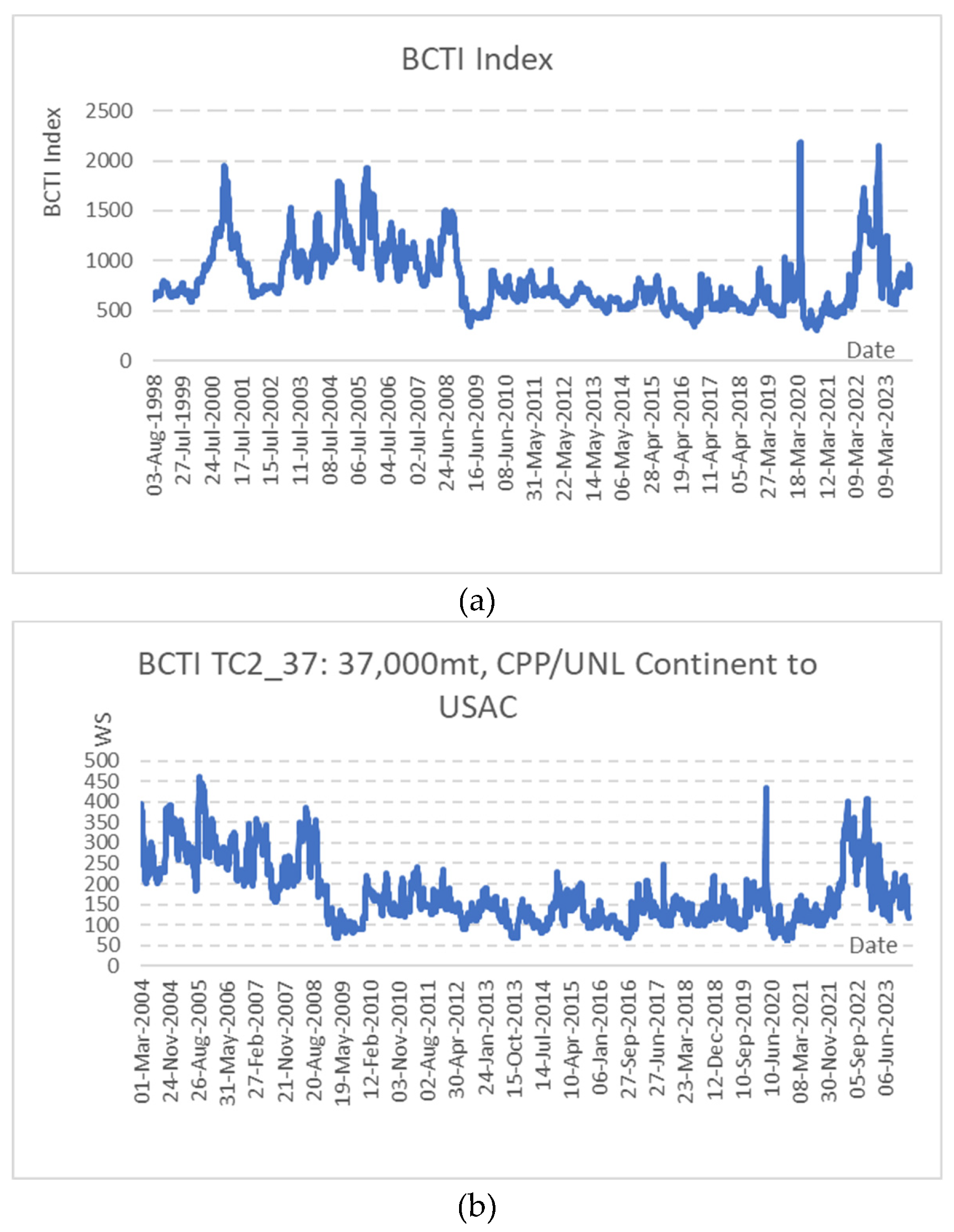
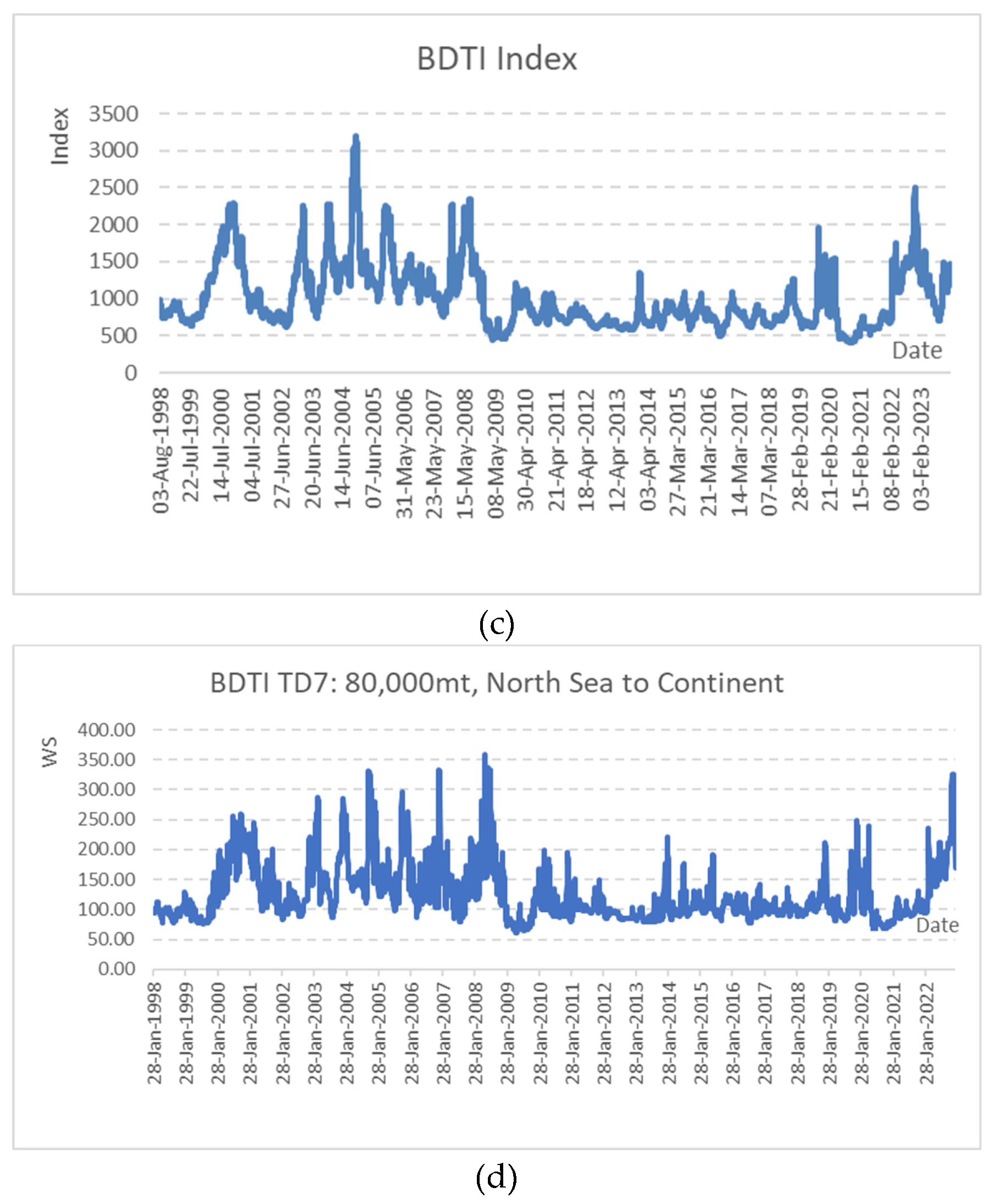
Figure 1 (a)-(d) describes the BCTI and BDTI of the sample observations. There are big volatilities in the year 2008 under global financial crisis, in the year 2020 when the COVID-19 break out and in the year 2022 when geographic conflict happened.
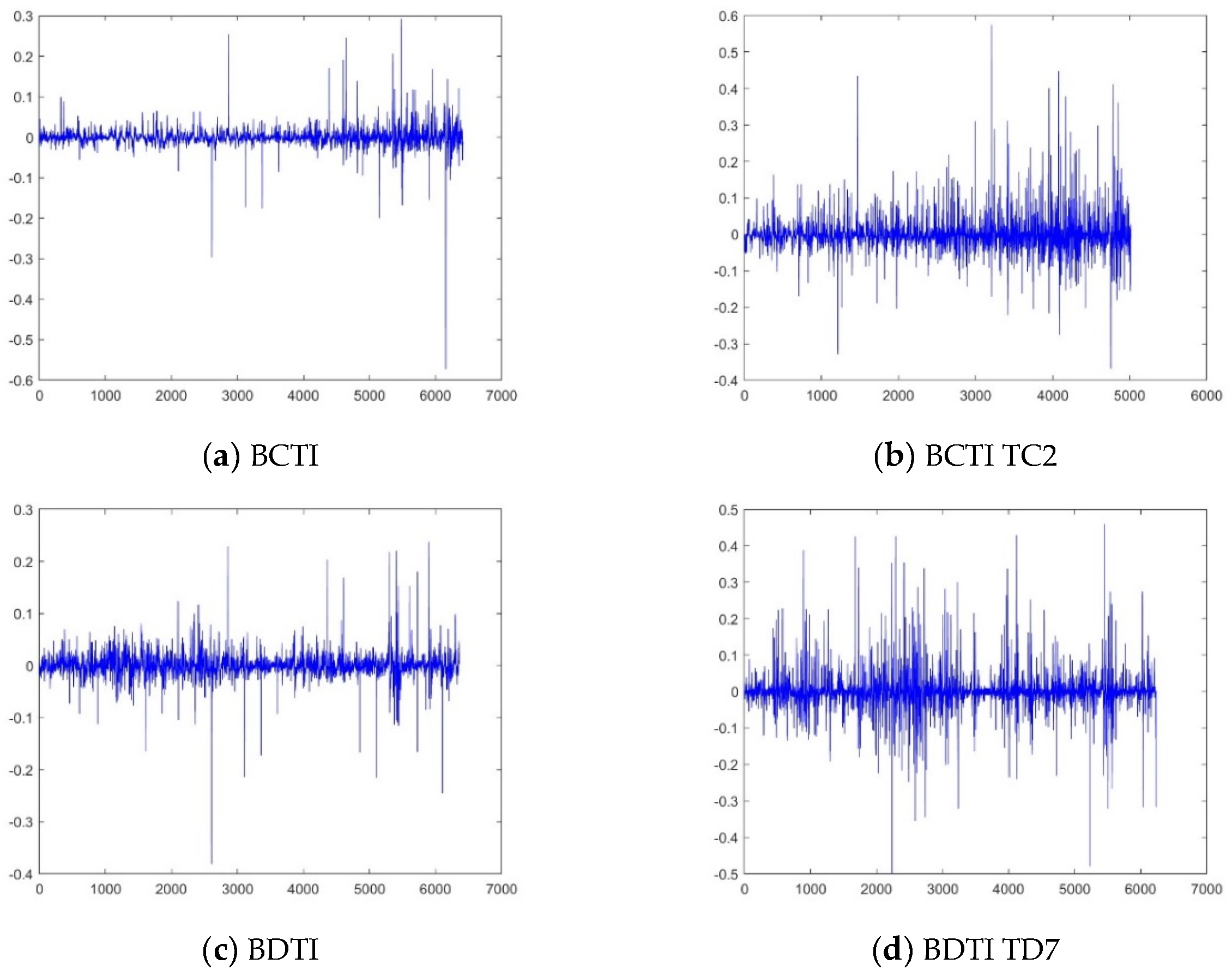
Figure 2 records the BCTI and BDTI logarithmic changes (that is,
), which is widely applied to calculate daily volatilities and the returns often help to decrease non-stationarities though it is not required in multifractal methods [
22,
23,
24].
4. Results and DISCUSSIONS
4.1. Multifractality in Dirty and Clean Tanker Freight Rate Returns
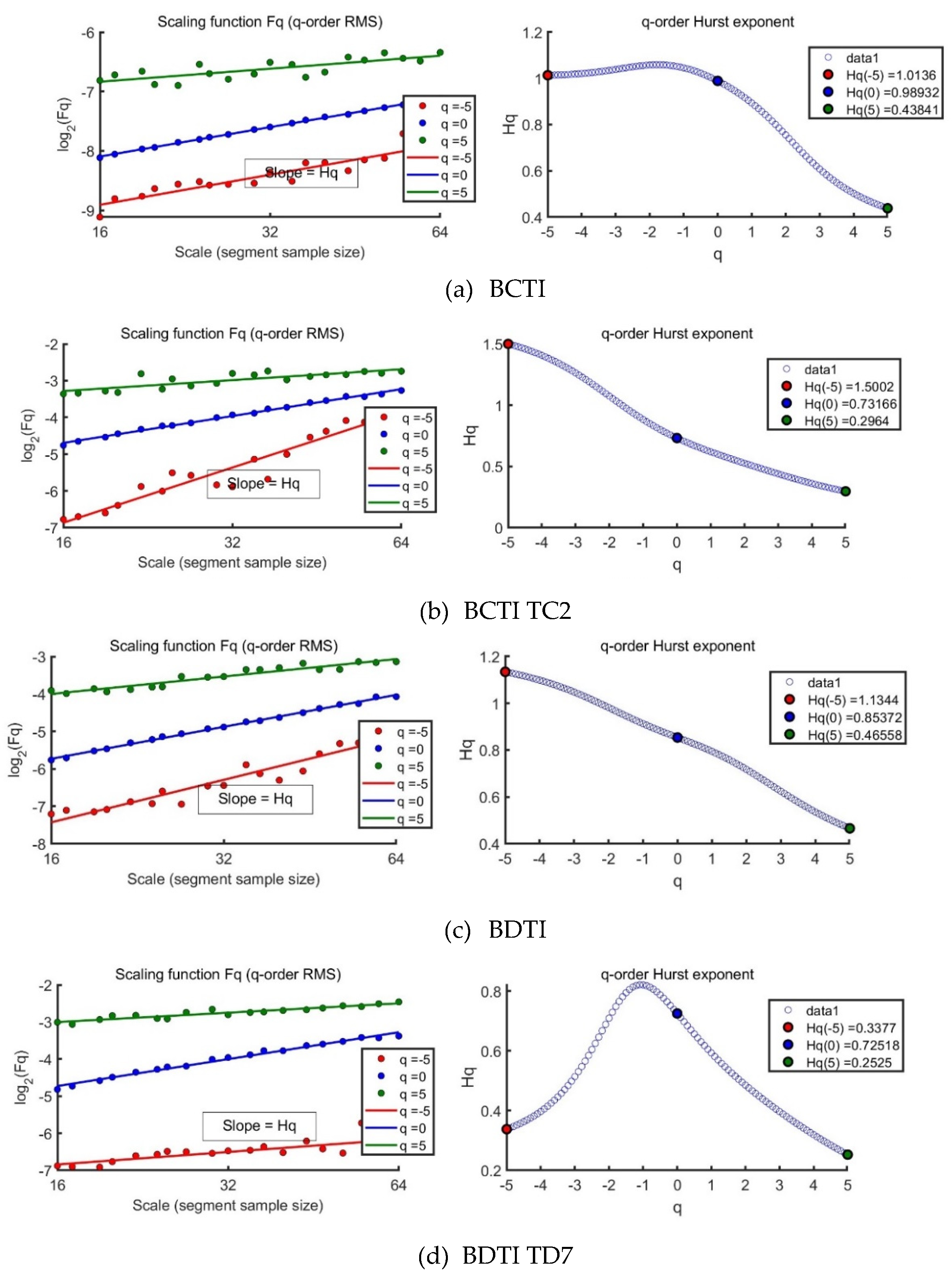
The Hurst exponent is a measure that characterizes the rate at which the root-mean-square (RMS) deviation of a time series expands as the size of the observational window (i.e., the scale) grows, revealing the monofractal nature of the data. In the context of a multifractal time series, the localized variations, or the RMS deviations, exhibit significantly large values for segments coinciding with periods of high fluctuation, and similarly, they show significantly small values for segments during periods of low fluctuation. The Hurst exponent is a measure used to characterize the fractal properties of a time series, indicating how the variance of the data changes with the scale of observation. For a monofractal time series, the Hurst exponent quantifies the rate at which the root-mean-square (RMS) error grows as the window breadth increases. In the context of multifractal time series, the local fluctuations are more complex. The local RMS fluctuation can be very large for segments that correspond to periods of high variability and very small for segments during periods of low variability. The
-order Hurst exponent is calculated by examining the slopes of the regression lines that relate the
-order RMS to the scale of the observation.
Figure 3(a) to (d) on the left illustrate that for multifractal time series, these slopes
vary depending on the value of
. The distinction between the
-order RMS for positive and negative fluctuations is more pronounced at smaller segment widths than at larger ones. This is because smaller segments are more sensitive to the local variability within a specific period, whereas larger segments encompass multiple periods and tend to average out the differences in fluctuation magnitude. As
increases, the
-order RMS for a multifractal time series generally decreases, as shown on the right side of
Figure 3(a) to (d). Both BCTI and BDTI returns exhibit multifractal characteristics, indicating that their fluctuation patterns are not uniform across different scales and require a more nuanced analysis to understand their underlying dynamics.
4.2. Multifractal Characteristics of Tanker Freight Fluctuation in Specific Routes
The logarithmic return of BCTI and BDTI and the specific routes in
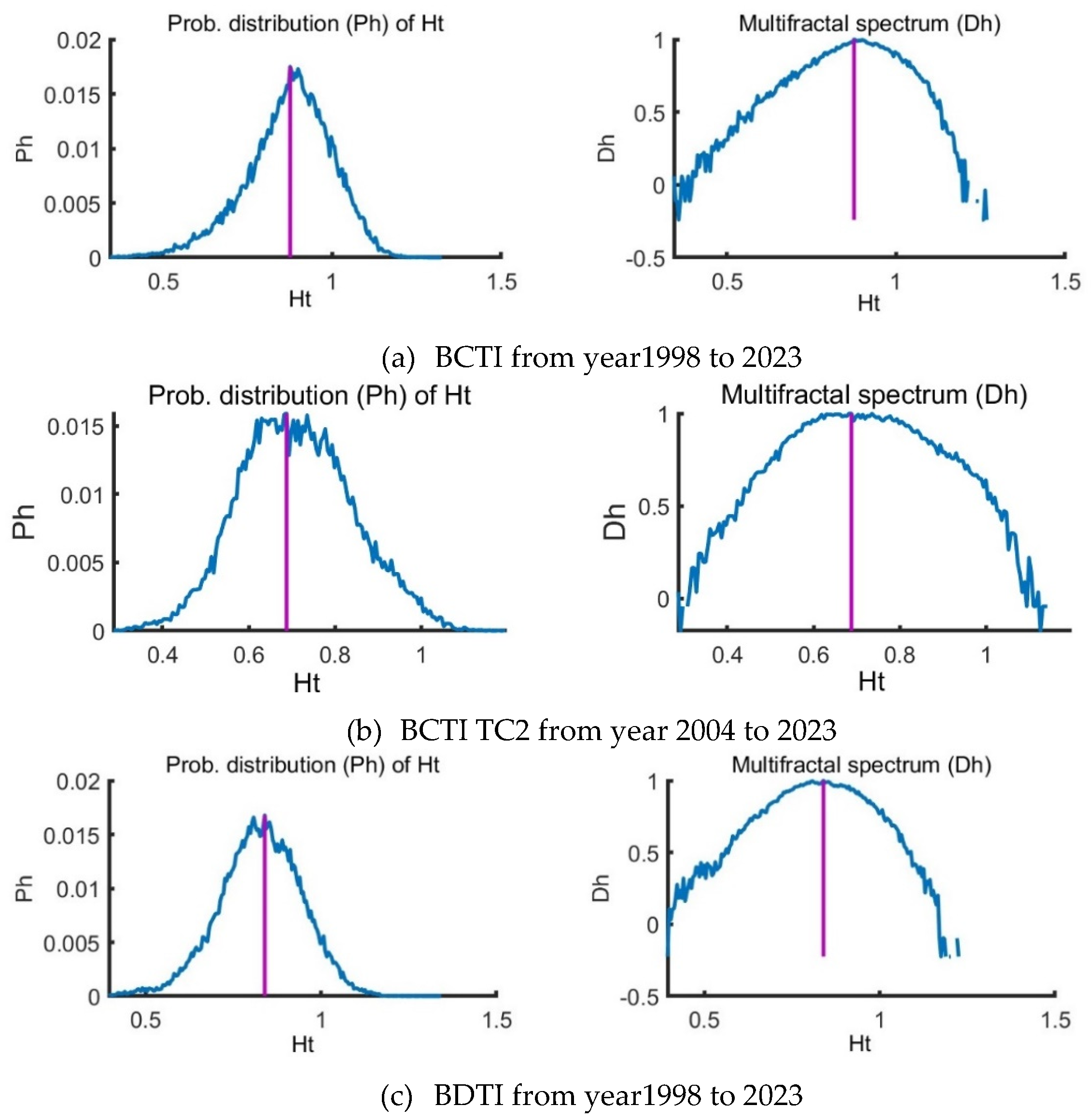
Figure 2 suggests that there exist big fluctuations in year 2008, year 2020 and year 2022 with events of financial crisis, COVID-19 and geographic conflict. From
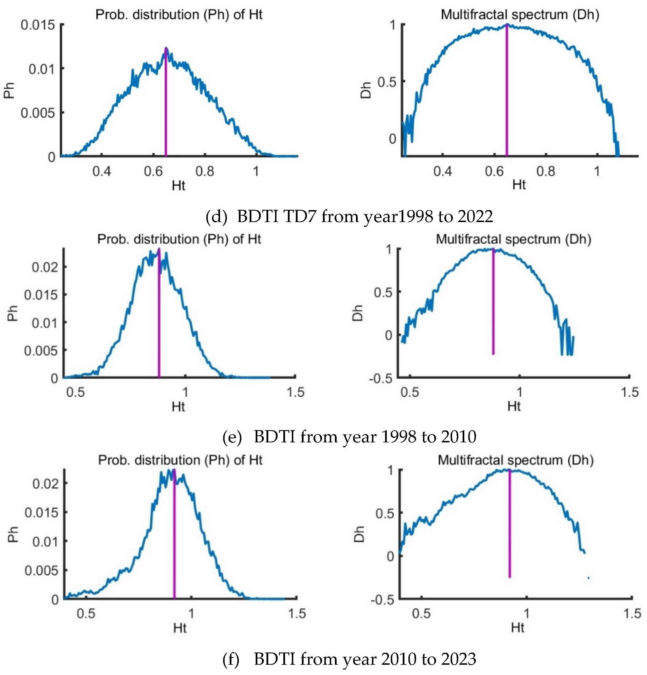
Figure 4 (a) and (c), both the BCTI and BDTI markets are with multifractal characteristics though they are different from the specific routes of TC2 and TD7 in
Figure 4 (b) and (d). According to references, big events such as global financial crisis can lead to structural breaks in time series [
44,
45,
46], we divide the sample data BDTI into two parts: period I from Jan 28, 1998 to Dec 01, 2010 and period II from Dec 02, 2010 to Jan 12, 2024 to delve into the changing external factors’ effects on the multifractalities.
The study of multifractal time series often involves various scaling exponents, among which the q-order Hurst exponent
is prominent. However, the local Hurst exponent
has proven advantageous in detecting specific time points of structural change within a time series [
44,
45,
46,
47,
48,
49,
50]. This local perspective aligns with q-order Hurst
values for extreme fluctuations, correlating positively or negatively depending on the q value's sign. The utility of the local Hurst exponent
is particularly evident when financial time series experience sudden disturbances. It pinpoints how these shocks modify the series' inherent scale-invariant features on a localized level. Visualized through histograms, the temporal variations of the local Hurst exponent
offer a probability distribution
of these changes (illustrated in
Figure 4 (e) for the first period and (f) for
the second period). Complementing this, the multifractal spectrum – delineated
by the parameters
f(
α) and
α – captures the
breadth of multifractality within the series (depicted in
Figure 4 (e) for the first period and (f) for
the second period). An increasing spectrum breadth denotes growing structural
disparities between periods marked by minor and major fluctuations. The
research employs multifractal spectrum width Δ
α as a measure of
multifractality level, which, according to results presented in
Figure 4 (e) and (f), confirms strong
multifractality in both examined periods of the Baltic Dry Index (BDTI)
returns. These findings align with previous research outlined in references [
40,
41,
42,
43], solidifying the observed characteristics of the market across different analytic methodologies.
4.3. Temporal Dynamics of Tanker Freight Market Complexity with MF-DMA Method
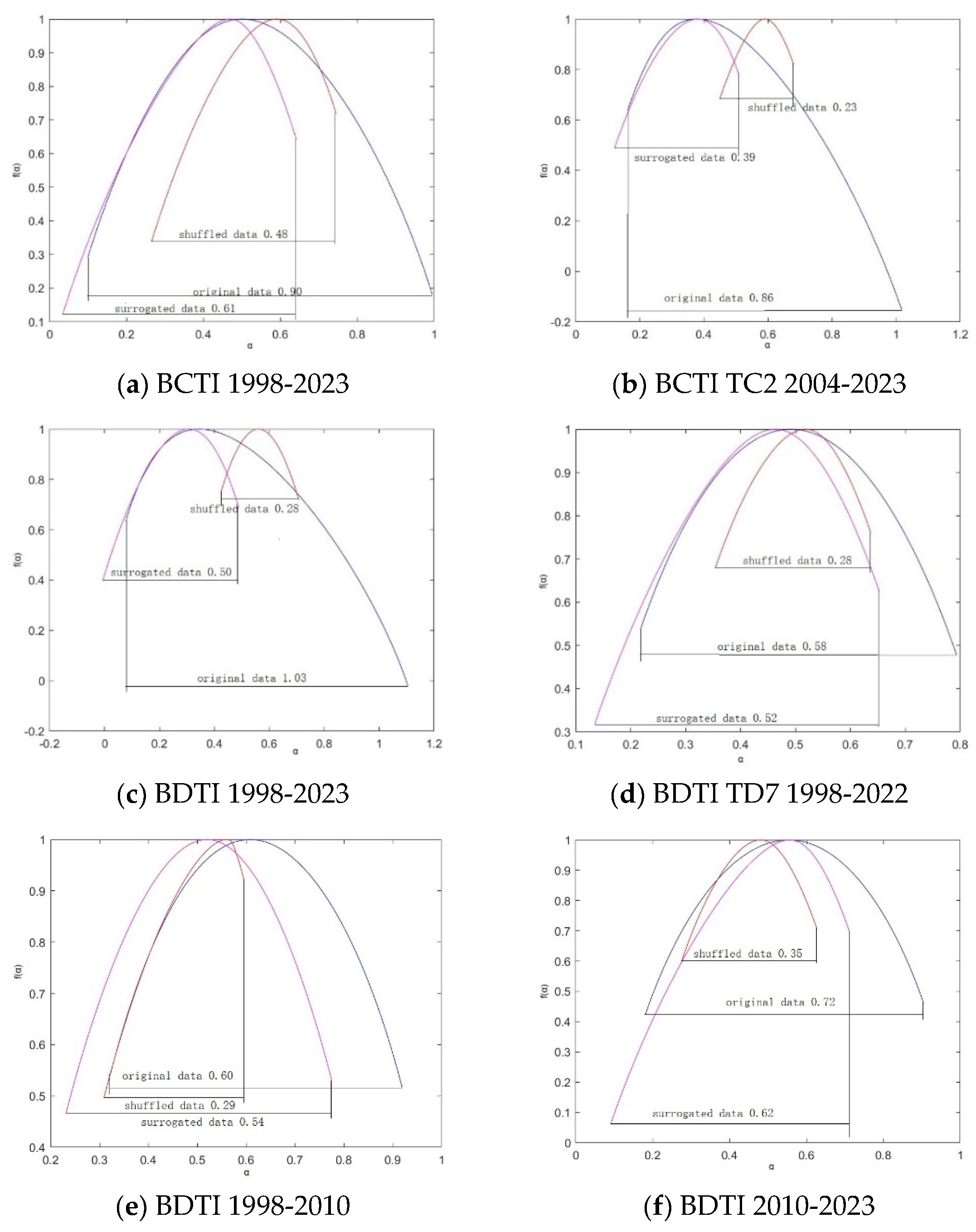
In
Figure 5 (a), the multifractality from PDF is
, while the total multifractality from the three parts is
. The multifractality from linear correlation and PDF are
, so the multifractality from the non-linear correlation
. The true multifractality
. The results in
Figure 5 (a)-(f) are listed in
Table 2.
The multifractality analysis of the Baltic Clean Tankers market in
Figure 5 (a) reveals significant insights into its dynamics. A multifractality value of 0.90 for the original data points to a highly complex market with pronounced multifractal behavior due to strong correlations at various time scales. A lesser, but still substantial, multifractality value of 0.61 in the surrogated data indicates that multifractality persists without temporal correlations, suggesting that price change distributions inherently contribute to market complexity. The shuffled data's multifractality value at 0.48, the lowest observed, illustrates the crucial role of temporal ordering in market behavior. These values collectively attest to the market's intricate and nonlinear interaction across scales.
The multifractality analysis for the Baltic Clean Tankers in
Figure 5 (a) and (b), inclusive of the specific 37000 tonnage route, elucidates distinct market dynamics. The original data for the entire market and the targeted route yield high multifractality values of 0.9 and 0.86 respectively, underscoring considerable multifractal behavior. However, subsequent surrogated and shuffled data yield diminished multifractality values of 0.61 and 0.48 for the broader market, and 0.39 and 0.23 for the specific route, respectively. These reductions upon data modification suggest inherent temporal organization as a key contributor to multifractality. The analysis underscores the influence of data structure on the assessment of market complexity and multifractal characteristics.
The multifractal analysis of the Baltic Dirty Tankers market data in
Figure 5 (c) reveals varying degrees of market complexity. An original multifractality value of 0.58 indicates a moderate complex market structure with self-similarity across time scales. The surrogated data's 0.52 multifractality value suggests that nontrivial scaling behavior persists even after the removal of some structural correlations. This denotes inherent complexity within the price change distribution itself. A notably lower multifractality value of 0.28 in the shuffled data emphasizes the importance of chronological order, indicating that temporal organization significantly contributes to the market’s multifractal nature.
The multifractal analysis for the Baltic Dirty Tankers market in a specific route TD7 at the 80000-tonnage level in
Figure 5 (d) exhibits a high degree of market complexity, with original data yielding a multifractality value of 1.03. This denotes a rich multifractal structure and extensive self-similarity across temporal scales. Upon surrogate treatment, multifractality is markedly reduced to 0.5, indicating a diminished multifractal behavior upon the exclusion of certain structural and temporal correlations. Further declines to a multifractality value of 0.28 in the shuffled data underscore the pivotal role of temporal sequencing in fostering multifractal properties.
4.4. A Comparison of the Multifractality Values for the Specified Periods of 1998 to 2010 and 2010 to 2023
The comparative assessment of the Baltic Dirty Tankers from the specified periods of 1998 to 2010 and 2010 to 2023 in
Figure 5 (e) and (f) may provide valuable insights into the temporal changes in multifractal nature and complexity within the market dynamics. The original multifractality value of 0.72 in the first period decreases to 0.60, suggesting a potential reduction in complexity and multifractal behavior. For the period of 1998 to 2010, the surrogated data yields a multifractality value of 0.62, indicating a decrease in complexity compared to the original data; similar for the period from 2010 to 2023. The shuffled data provides additional insights into the temporal changes in multifractality. For the period of 1998 to 2010, the shuffled data yields a multifractality value of 0.35, reflecting a notable reduction in complexity compared to the original and surrogated data. Likewise, for the period from 2010 to 2023, the value further decreases to 0.29, signaling a continued decrease in complexity during the later period. Overall, the period from 1998 to 2010 exhibits higher multifractality values across all data types, indicating stronger multifractal nature and greater complexity.
The changes in multifractality values for the Baltic Dirty Tankers market between the periods of 1998 to 2010 and 2010 to 2023 may reflect several major factors that influenced the market dynamics. Some of the potential factors that could have affected trading patterns are listed in
Table 3. These potential factors indicate the complex and multifaceted nature of the changes in the tanker market across the two time periods, offering valuable insights into the Baltic Dirty Tankers market's evolving complexity.
The multifractality comparison between the periods from 1998 to 2010 and 2010 to 2023 in the Baltic Dirty Tankers market reveals intriguing insights. From 1998 to 2010, the market exhibited higher complexity with a multifractality value of 0.72, reflecting the impact of the 2008 Financial Crisis. In contrast, the period from 2010 to 2023, despite various influential factors, such as Diversification of Trade Routes, Technology Integration, Eco-Friendly Practices, and Geopolitical Developments, shows lower multifractality values, indicating decreased complexity and non-linear dynamics. This shift signifies a transition from crisis-driven complexity to a phase shaped by diverse influences, despite continued market intricacy. The multifractality analysis captures the nuanced evolution of market complexity, reflecting the changing nature of multifractal behavior.
4.5. Discussion
In
Table 2, there is an interesting result of the effective multifractality of the BDTI (
) and two periods (
). When we cut the sample of BDTI into two parts, the effective multifractality is cut into two parts, which means that each period may exhibit its own multifractal characteristics. These could differ due to several reasons such as changes in market regulations, economic shifts, or even technological innovations that affect the market dynamics. The multifractal analysis for each period may reveal different levels of market complexity, structural breaks, variability in investment strategies and adaptive market hypothesis.
5. Conclusions
This study utilizes MF-DMA methodology to unravel the multifaceted nature of the Baltic Tanker freight market. Initial findings suggest an overarching multifractal nature within the market, with total multifractality reaching up to 0.90 in the Clean Tankers market. This complexity is partly from both a fat-tailed probability distribution 0.48 and non-linear correlations 0.29, indicating sophisticated temporal organization and inherent volatility as core components of market behavior. A closer examination of a specific route TC2 with the 37000 tonnage, the market retains its multifractal attributes albeit with reduced magnitudes upon data manipulation. This consistent reduction in multifractality values—evident upon shuffling and surrogating—reinforces the significant contribution of temporal arrangement to the market's complex structure.
In the case of the Dirty Tankers market, the study signifies a moderate complexity with an original multifractality value of 0.58, which diminishes under surrogate and shuffled scenarios, implying that chronological sequencing is crucial for preserving the multifractal properties within this segment. This assertion is further substantiated when focusing on specific routes like TD7 at the 80000-tonnage level, where multifractality peaks at 1.03 yet declines markedly when temporal and structural correlations are disrupted. Comparatively, multifractal dynamics transition between the two periods under investigation - higher multifractality in the earlier period (1998-2010) underscores a phase influenced significantly by the 2008 Financial Crisis, while the subsequent era (2010-2023) showcases a dampening of complexity. This suggests a shift from an environment dominated by crisis-induced market behaviors to one where multifractal measure have adapted to diverse and modern market forces, including technological advancements, regulatory changes, and environmental dynamics.
In conclusion, the multifractal analysis offers a comprehensive framework for fleet managers and energy importers to proactively prepare for and navigate the complexities of the tanker market. By implementing measures such as diversifying trade routes, embracing technological innovations, prioritizing eco-friendly practices, developing robust risk management strategies, engaging with regulatory bodies, leveraging market intelligence, and investing in talent development, stakeholders can enhance operational resilience, fortify their competitive position, and navigate the intricacies of the tanker industry with greater agility and foresight. These strategic endeavors underscore the imperative of proactive preparedness and adaptive capacity in addressing the evolving challenges and opportunities within the tanker market, thereby contributing to sustained operational excellence and strategic advantage.
The cutting multifractality of BDTI in two different time windows needs more investigation when the empirical data is available. This may give insights to discuss how the complex dynamics of the system might vary over time.
Author Contributions
Conceptualization, F.C.; methodology, F.C.; software, F.C.; validation, X.L. and F.C.; formal analysis, F.C.; investigation, F.C.; resources, X.L.; data curation, X.L.; writing—original draft preparation, F.C.; writing—review and editing, X.L.; visualization, X.L.; supervision, F.C.; project administration, F.C.; funding acquisition, F.C. All authors have read and agreed to the published version of the manuscript.
Funding
This research was funded by the National Social Science Fund of China, grant number 23BJL020 and the APC was funded by it.
Data Availability Statement
Acknowledgments
We appreciate the help from the editorial office, the reviewers’ valuable comments and the Editor’s guidance to improve our manuscript.
Conflicts of Interest
The authors declare no conflicts of interest. The funders had no role in the design of the study; in the collection, analyses, or interpretation of data; in the writing of the manuscript; or in the decision to publish the results.
References
- Mantegna, R.N.; Stanley, H.E. Scaling behaviour in the dynamics of an economic index. Nature 1995, 376, 46–49. [Google Scholar] [CrossRef]
- Mantegna, R.N.; Stanley, H.E. An Introduction to Econophysics; Cambridge University Press: Cambridge, UK, 1999. [Google Scholar] [CrossRef]
- Bouchaud, J.P.; Potters, M. ; Theory of Financial Risk; Cambridge University Press: Cambridge, UK, 2000. [Google Scholar]
- Drożdż, S.; Kwapień, J.; Oświecimka, P.; Rak, R. Quantitative features of multifractal subtleties in time series. EPL Europhysics Lett. 2009, 88, 60003. [Google Scholar] [CrossRef]
- Zhou, W.-X. Finite-size effect and the components of multifractality in financial volatility. Chaos, Solitons Fractals 2012, 45, 147–155. [Google Scholar] [CrossRef]
- Di Matteo, A.; Pirrotta, A. Generalized differential transform method for nonlinear boundary value problem of fractional order. Commun. Nonlinear Sci. Numer. Simul. 2015, 29, 88–101. [Google Scholar] [CrossRef]
- Grech, D. Chaos, Alternative measure of multifractal content and its application in finance. Solitons Fractals 2016, 88, 183–195. [Google Scholar] [CrossRef]
- Li, K.X.; Xiao, Y.; Chen, S.-L.; Zhang, W.; Du, Y.; Shi, W. Dynamics and interdependencies among different shipping freight markets. Marit. Policy Manag. 2018, 45, 837–849. [Google Scholar] [CrossRef]
- Khan, K.; Su, C.W.; Tao, R.; Umar, M. How often do oil prices and tanker freight rates depend on global uncertainty? Reg. Stud. Mar. Sci. 2021, 48. [Google Scholar] [CrossRef]
- Zhang, J.; Zeng, Q. Modelling the volatility of the tanker freight market based on improved empirical mode decomposition. Appl. Econ. 2017, 49, 1655–1667. [Google Scholar] [CrossRef]
- Abouarghoub, W.; Nomikos, N.K.; Petropoulos, F. On reconciling macro and micro energy transport forecasts for strategic decision making in the tanker industry. Transp. Res. Part E: Logist. Transp. Rev. 2018, 113, 225–238. [Google Scholar] [CrossRef]
- Zhang, X.; Podobnik, B.; Kenett, D.Y.; Stanley, H.E. Systhmic Risk and Causality Dynamics of the World International Shipping Market. Physic A 2014, 415, 43–53. [Google Scholar] [CrossRef]
- Bai, X. Tanker freight rates and economic policy uncertainty: A wavelet-based copula approach. Energy 2021, 235, 121383. [Google Scholar] [CrossRef]
- Mandelbrot, B.B. The Fractal Geometry of Nature; Freeman: New York, NY, USA, 1982. [Google Scholar]
- Lloyd, E.H.; Hurst, H.E.; Black, R.P.; Simaika, Y.M. Long-Term Storage: An Experimental Study. J. R. Stat. Soc. Ser. A (General) 1965, 129, 591. [Google Scholar] [CrossRef]
- Castro e Silva, J.G. Moreira, Roughness exponents to calculate multi-affine fractal exponents. Phys. A 1997, 235, 327–333. [Google Scholar] [CrossRef]
- Peng, C.-K.; Havlin, S.; Stanley, H.E.; Goldberger, A.L. Quantification of Scaling Exponents and Crossover Phenomena in Nonstationary Heartbeat Time Series. CHAOS 1995, 5, 82–87. [Google Scholar] [CrossRef] [PubMed]
- Yamasaki, K.; Muchnik, L.; Havlin, S.; Bunde, A.; Stanley, H.E. Scaling and memory in volatility return intervals in financial markets. Proc. Natl. Acad. Sci. USA 2005, 102, 9424–9428. [Google Scholar] [CrossRef]
- Green, E.; Hanan, W.; Heffernan, D. The origins of multifractality in financial time series and the effect of extreme events. Eur. Phys. J. B 2014, 87, 1–9. [Google Scholar] [CrossRef]
- Kantelhardt, J.W.; Zschiegner, S.A.; Koscielny-Bunde, E.; Havlin, S.; Bunde, A.; Stanley, H. Multifractal detrended fluctuation analysis of nonstationary time series. Phys. A: Stat. Mech. its Appl. 2002, 316, 87–114. [Google Scholar] [CrossRef]
- Ihlen, E.A.F. Introduction to Multifractal Detrended Fluctuation Analysis in Matlab. Front. Physiol. 2012, 3, 141. [Google Scholar] [CrossRef]
- Chen, F.; Miao, Y.; Tian, K.; Ding, X.; Li, T. Multifractal cross-correlations between crude oil and tanker freight rate. Phys. A: Stat. Mech. its Appl. 2017, 474, 344–354. [Google Scholar] [CrossRef]
- Czarnecki. ; Grech, D. Multifractal Dynamics of Stock Markets. Acta Phys. Pol. A 2010, 117, 623–629. [Google Scholar] [CrossRef]
- Grech, D.; Pamuła, G. On the multifractal effects generated by monofractal signals. Phys. A: Stat. Mech. its Appl. 2013, 392, 5845–5864. [Google Scholar] [CrossRef]
- Arianos, S.; Carbone, A. Detrending moving average algorithm: A closed-form approximation of the scaling law[J]. Phys. A: Stat. Mech. Its Appl. 2007, 382, 9–15. [Google Scholar] [CrossRef]
- Gu G F, Zhou W X. Detrending moving average algorithm for multifractals[J]. Phys. Rev. E 2010, 82, 011136. [Google Scholar] [CrossRef]
- Kwapień, J.; Blasiak, P.; Drożdż, S.; Oświęcimka, P. Genuine multifractality in time series is due to temporal correlations. Phys. Rev. E 2023, 107, 034139. [Google Scholar] [CrossRef]
- Mantegna, R.N.; Stanley, H.E. Turbulence and financial markets. Nature 1996, 383, 587–588. [Google Scholar] [CrossRef]
- Stanley, H.E.; Gabaix, X.; Gopikrishnan, P.; Plerou, V. Economic Fluctuations and Statistical Physics: The Puzzle of Large Fluctuations. Nonlinear Dyn. 2006, 44, 329–340. [Google Scholar] [CrossRef]
- Bai, X.; Lam, J.S.L. Freight rate co-movement and risk spillovers in the product tanker shipping market: A copula analysis. Transp. Res. Part E: Logist. Transp. Rev. 2021, 149, 102315. [Google Scholar] [CrossRef]
- Chen, J.; Zhao, R.; Xiong, W.; Wan, Z.; Xu, L.; Zhang, W. Influencing factors of crude oil maritime shipping freight fluctuations: a case of Suezmax tankers in Europe–Africa routes. Marit. Bus. Rev. 2023, 8, 48–64. [Google Scholar] [CrossRef]
- Dai, L.; Hu, H.; Tao, Y.; Lee, S. The volatility transmission between crude oil market and tanker freight market. Int. J. Shipp. Transp. Logist. 2020, 12, 619–634. [Google Scholar] [CrossRef]
- Gavalas, D.; Syriopoulos, T.; Tsatsaronis, M. COVID–19 impact on the shipping industry: An event study approach. Transp. Policy 2022, 116, 157–164. [Google Scholar] [CrossRef]
- Gavriilidis, K.; Kambouroudis, D.S.; Tsakou, K.; Tsouknidis, D.A. Volatility forecasting across tanker freight rates: The role of oil price shocks. Transp. Res. Part E: Logist. Transp. Rev. 2018, 118, 376–391. [Google Scholar] [CrossRef]
- Khan, K.; Su, C.W.; Khurshid, A.; Umar, M. The dynamic interaction between COVID-19 and shipping freight rates: a quantile on quantile analysis. Eur. Transp. Res. Rev. 2022, 14, 1–16. [Google Scholar] [CrossRef]
- Michail, N.A.; Melas, K.D. Quantifying the relationship between seaborne trade and shipping freight rates: A Bayesian vector autoregressive approach. Marit. Transp. Res. 2020, 1, 100001. [Google Scholar] [CrossRef]
- Michail, N.A.; Melas, K.D. Shipping markets in turmoil: An analysis of the Covid-19 outbreak and its implications. Transp. Res. Interdiscip. Perspect. 2020, 7, 100178–100178. [Google Scholar] [CrossRef]
- Michail, N.A.; Melas, K.D. Covid-19 and the energy trade: Evidence from tanker trade routes. Asian J. Shipp. Logist. 2022, 38, 51–60. [Google Scholar] [CrossRef]
- Regli, F.; Nomikos, N.K. The eye in the sky – Freight rate effects of tanker supply. Transp. Res. Part E: Logist. Transp. Rev. 2019, 125, 402–424. [Google Scholar] [CrossRef]
- Shi, W.; Li, K.X.; Yang, Z.; Wang, G. Time-varying copula models in the shipping derivatives market. Empir. Econ. 2017, 53, 1039–1058. [Google Scholar] [CrossRef]
- Siddiqui, A.W.; Basu, R. An empirical analysis of relationships between cyclical components of oil price and tanker freight rates. Energy 2020, 200, 117494. [Google Scholar] [CrossRef]
- Zhang, X.; Bao, Z.; Ge, Y.-E. Investigating the determinants of shipowners’ emission abatement solutions for newbuilding vessels. Transp. Res. Part D: Transp. Environ. 2021, 99, 102989. [Google Scholar] [CrossRef]
- Zhang, Y.; Lam, J.S.L. Investigating dependencies among oil price and tanker market variables by copula-based multivariate models. Energy 2018, 161, 435–446. [Google Scholar] [CrossRef]
- Buonocore, R.; Aste, T.; Di Matteo, T. Measuring multiscaling in financial time-series. Chaos, Solitons Fractals 2016, 88, 38–47. [Google Scholar] [CrossRef]
- Chen, F.; Tian, K.; Ding, X.; Li, T.; Miao, Y.; Lu, C. Multifractal characteristics in maritime economics volatility. Int. J. Transp. Econ. 2017, 44, 365–380. [Google Scholar]
- Vogl, M. Controversy in financial chaos research and nonlinear dynamics: A short literature review. Chaos, Solitons Fractals 2022, 162, 112444. [Google Scholar] [CrossRef]
- Press, W.H.; Teukolsky, S.A.; Vetterling, W.T.; Flannery, B.P. Numerical Recipes in FORTRAN: The Art of Scientific Computing, 2nd ed.; Cambridge University Press: New York, NY, USA, 1996. [Google Scholar]
- Grobys, K. A multifractal model of asset (in)variances. J. Int. Financial Mark. Institutions Money 2023, 85. [Google Scholar] [CrossRef]
- Schumann, A.Y.; Kantelhardt, J.W. Multifractal moving average analysis and test of multifractal model with tuned correlations. Phys. A: Stat. Mech. its Appl. 2011, 390, 2637–2654. [Google Scholar] [CrossRef]
- Manimaran, P.; Panigrahi, P.K.; Parikh, J.C. Multiresolution analysis of fluctuations in non-stationary time series through discrete wavelets. Phys. A: Stat. Mech. its Appl. 2009, 388, 2306–2314. [Google Scholar] [CrossRef]
- Li, Q.; Fu, Z.; Yuan, N.; Xie, F. Effects of non-stationarity on the magnitude and sign scaling in the multi-scale vertical velocity increment. Phys. A: Stat. Mech. its Appl. 2014, 410, 9–16. [Google Scholar] [CrossRef]
- Halsey, T.C.; Jensen, M.H.; Kadanoff, L.P.; Procaccia, I.; Shraiman, B.I. Fractal measures and their singularities: the characterization of strange sets. Phys. Rev. A 1986, 33, 1141–1151. [Google Scholar] [CrossRef]
- Zhou, W.-X. The components of empirical multifractality in financial returns. EPL (Europhysics Lett. 2009, 88, 28004. [Google Scholar] [CrossRef]
- Schreiber, T.; Schmitz, A. Improved Surrogate Data for Nonlinearity Tests. Phys. Rev. Lett. 1996, 77, 635–638. [Google Scholar] [CrossRef] [PubMed]
- Jiang, Z.-Q.; Xie, W.-J.; Zhou, W.-X.; Sornette, D. Multifractal analysis of financial markets: a review. Rep. Prog. Phys. 2019, 82, 125901. [Google Scholar] [CrossRef]
- Li, Y.; Yin, M.; Khan, K.; Su, C.-W. The impact of COVID-19 on shipping freights: asymmetric multifractality analysis. Marit. Policy Manag. 2023, 50, 889–907. [Google Scholar] [CrossRef]
- Martínez, J.L.M.; Segovia-Domínguez, I.; Rodríguez, I.Q.; Horta-Rangel, F.A.; Sosa-Gómez, G. A modified Multifractal Detrended Fluctuation Analysis (MFDFA) approach for multifractal analysis of precipitation. Phys. A: Stat. Mech. its Appl. 2021, 565, 125611. [Google Scholar] [CrossRef]
- Rak, R.; Grech, D. Quantitative approach to multifractality induced by correlations and broad distribution of data. Phys. A: Stat. Mech. its Appl. 2018, 508, 48–66. [Google Scholar] [CrossRef]
|
Disclaimer/Publisher’s Note: The statements, opinions and data contained in all publications are solely those of the individual author(s) and contributor(s) and not of MDPI and/or the editor(s). MDPI and/or the editor(s) disclaim responsibility for any injury to people or property resulting from any ideas, methods, instructions or products referred to in the content. |
© 2024 by the authors. Licensee MDPI, Basel, Switzerland. This article is an open access article distributed under the terms and conditions of the Creative Commons Attribution (CC BY) license (http://creativecommons.org/licenses/by/4.0/).


