Submitted:
08 March 2024
Posted:
08 March 2024
You are already at the latest version
Abstract
Keywords:
1. Introduction
2. DeepOnet Algorithm and Modeling
3. Results and Analysis
3.1. Hyperparameters Tuning for DeepOnet and LSTM Models
3.2. Multi-Steps Prediction by DeepOnet and LSTM Models
4. Conclusion
Author Contributions
Funding
Data Availability Statement
Conflicts of Interest
References
- Triantafyllou M., Bodson M., Athans M. Real time estimation of ship motions using Kalman filtering techniques. IEEE Journal of Oceanic Engineering1983, 8(1), 9-20 . [CrossRef]
- Peng X.Y., Dong H. Y., Zhang B. Echo state network ship motion modeling prediction based on Kalman filter. 2017 IEEE International Conference on Mechatronics and Automation (ICMA)2017,95-100 .
- Haiping Fan. Study on the prediction and Estimation of Ship Roll Motion Based on Kalman Filter. Harbin Engineering University 2008, 6-35.[in Chinese] .
- Zhonghua Zhang, Mengda Wu. Time-Sequence Method for the Real-Time Filtering and Prediction of the Ship-Swaying Data. Journal of Chinese Inertial Technology 2000, 04, 25-31. [in Chinese] .
- Suhermi N., Suhartono, Prastyo D. D., Ali B. Roll motion prediction using a hybrid deep learning and ARIMA model. Procedia Computer Science 2018, 144, 251-258 . [CrossRef]
- Likun Li. Directional spectral estimation of ship motion based on parameter method. Ship Science and Technology 2017, 39(1), 10-12. [in Chinese] .
- Duan W., Huang L., Han Y. A hybrid AR-EMD-SVR model for the short-term prediction of nonlinear and non-stationary ship motion. Journal of Zhejiang University Science 2015, A16 (7), 562-576 .
- Zeng B, Liu S.A self-adaptive intelligence gray prediction model with the optimal fractional order accumulating operator and its application. Mathematical Methods in the Applied Sciences 2017,40(18),7843-7857 . [CrossRef]
- Min Gu, Changde Liu, Jinfeng Zhang. Extreme short-term prediction of ship motion based on chaotic theory and RBF neural network. Ship mechanics 2013, 17(10), 1147-1152. [in Chinese] .
- Yin J. C., Wang L. D, Wang N.N. Avariable-structure gradient RBF network with its application to predictive ship motion control. Asian Journal of Control 2012,14,716-725 .
- Yin J. C., Perakis A.N, Wang N. A real-time ship roll motion prediction using wavelet transform and variable RBF network. Ocean Engineering 2018,160,10-19 .
- Wanting Liu. Study on Heave Motion Prediction od Ship. Dalian Maritime University 2016, 7-28. [in Chinese] .
- Li X., Lv X., Yu J., Li J. Neural network application on ship motion prediction. Proceedings of 9th International Conference on Intelligent Human-Machine Systems and Cybernetics, Hangzhou 2017, 414-417 .
- Guodong Wang. Short-term Prediction and simulation of Ship’s Moyion Based onLSTM. Jiangsu university of science and technology 2017, 8-46. [in Chinese] .
- Ni C, Ma X. An integrated long-short term memory algorithm for predicting polar westerlies wave height. Ocean Engineering 2020, 215(1):107715 . [CrossRef]
- Y Zhao, Dan Su. Rogue Wave Prediction Based on Four Combined Long Short-Term Memory Neural Network Models, Journal of Shanghai Jiao tong University 2022, 56(04), 516-522. [in Chinese] .
- Y Zhao, Dan Su. Rogue wave prediction based on LSTM neural network, Journal of Huazhong University of Science and Technology (Natural Science Edition) 2020, 48(7), 47-51. [in Chinese] .
- Yue Liu, Xiantao Zhang, Gang Chen, Qing Dong, Xiaoxian Guo, Xinliang Tian, Wenyue Lu, Tao Peng, Deterministic wave prediction model for irregular long‐crested waves with Recurrent Neural Network, Journal of Ocean Engineering and Science 2022. [CrossRef]
- Sun Q, Tang Z, Gao J,et al. Short-term ship motion attitude prediction based on LSTM and GPR. Applied Ocean Research 2022, (118-):118 .
- Han C, Hu X. A Prediction Method of Ship Motion Based on LSTM Neural Network with Variable Step-Variable Sampling Frequency Characteristics. Journal of Marine Science and Engineering 2023, 11(5):919 . [CrossRef]
- Ling Liu, Yu Yang, Tao Peng, Machine learning prediction of 6-DOF motions of KVLCC2 ship based on RC model, Journal of Ocean Engineering and Science 2022. [CrossRef]
- Hou X, Xia S. Short-Term Prediction of Ship Roll Motion in Waves Based on Convolutional Neural Network. Journal of Marine Science and Engineering 2024, 12(1):102 . [CrossRef]
- Wenhai Yi, Zhiliang Gao. Very Short-term Prediction of ship Rolling Motion in Random Transverse Waves Based on LSTM Neural Network. Journal of Wuhan University of Technology: Transportation Science and Engineering Edition 2021, 45(6):5. [in Chinese] .
- Ferrandis JDG, Triantafyllou MS, Chryssostomidis C, et al. Learning functionals via LSTM neural networks for predicting vessel dynamics in extreme sea states. Proceedings of The Royal Society A Mathematical Physical and Engineering Sciences 2021, 477(2245), 20190897 . [CrossRef]
- Lu, L., Jin, P., Pang, G. et al. Learning nonlinear operators via DeepONet based on the universal approximation theorem of operators. Nature Machine Intelligence 2021, 3, 218–229 . [CrossRef]
- Jr M I, Longo J, Stern F. Pitch and Heave Tests and Uncertainty Assessment for a Surface Combatant in Regular Head Waves. Journal of Ship Research 2008, 52(2), 146-163 .
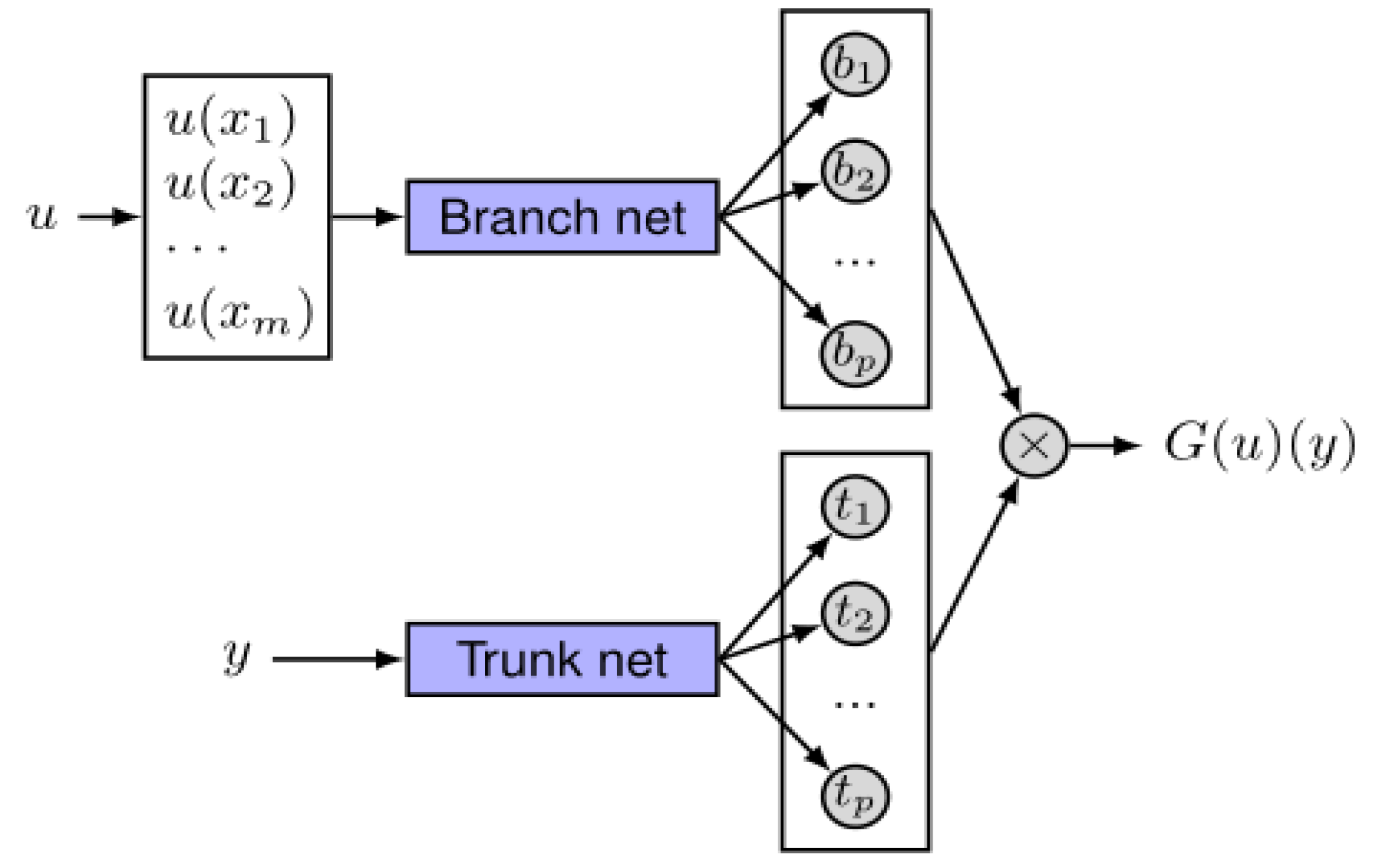
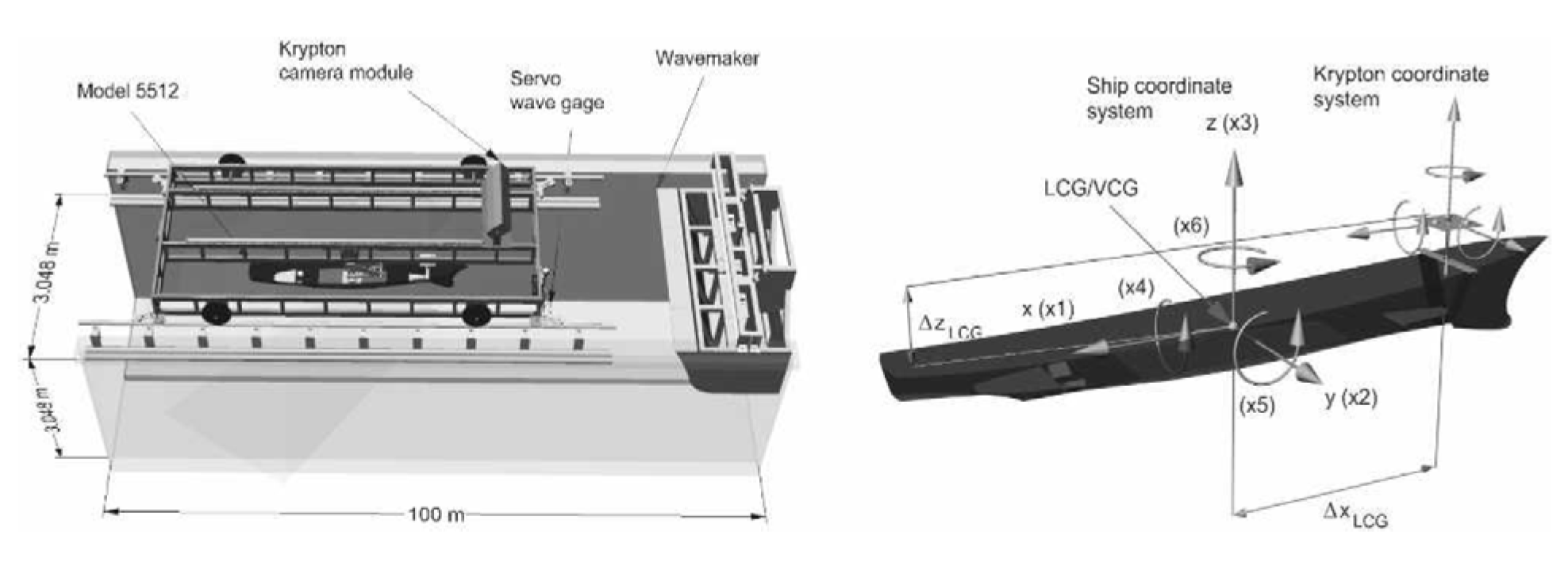
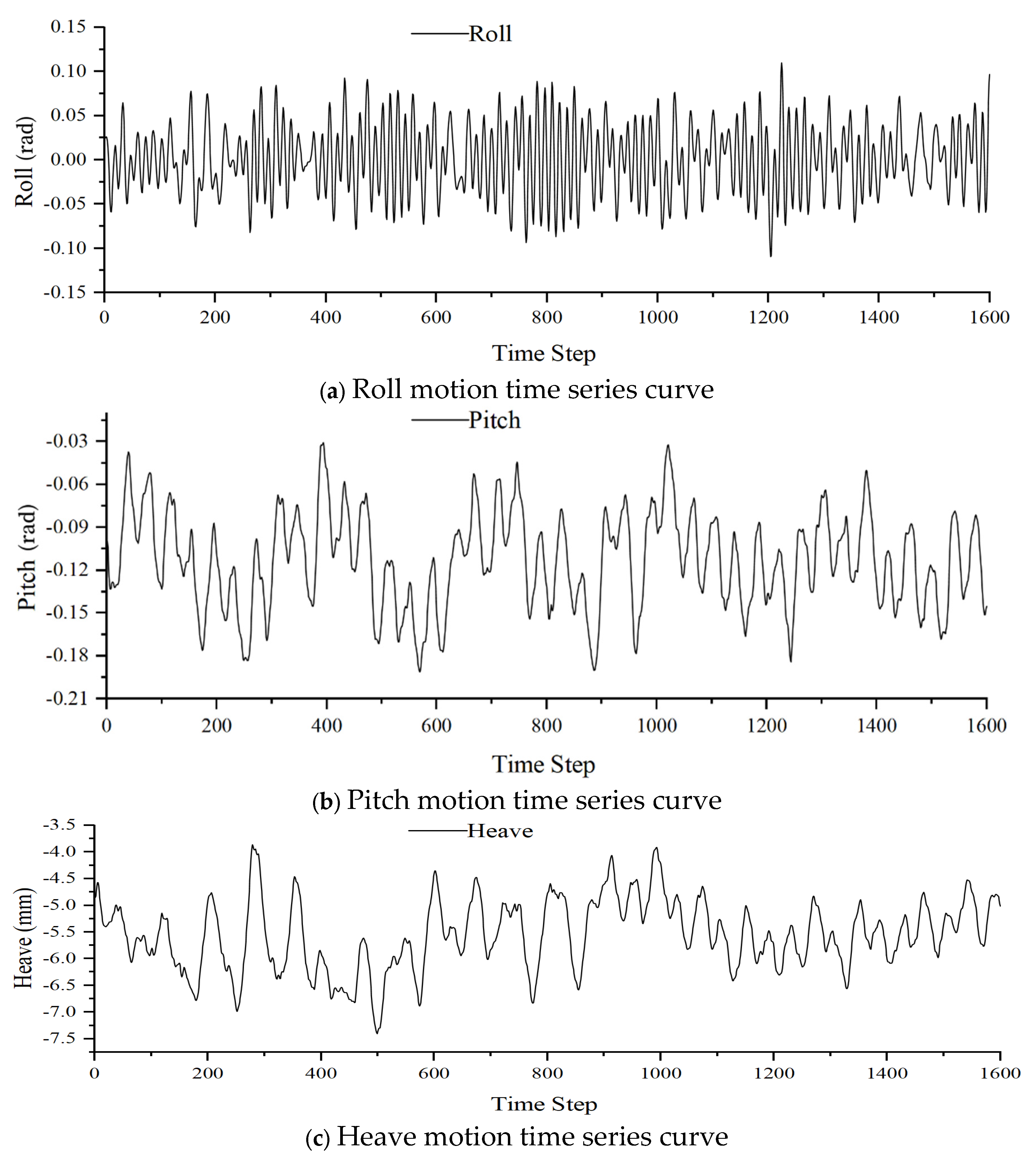
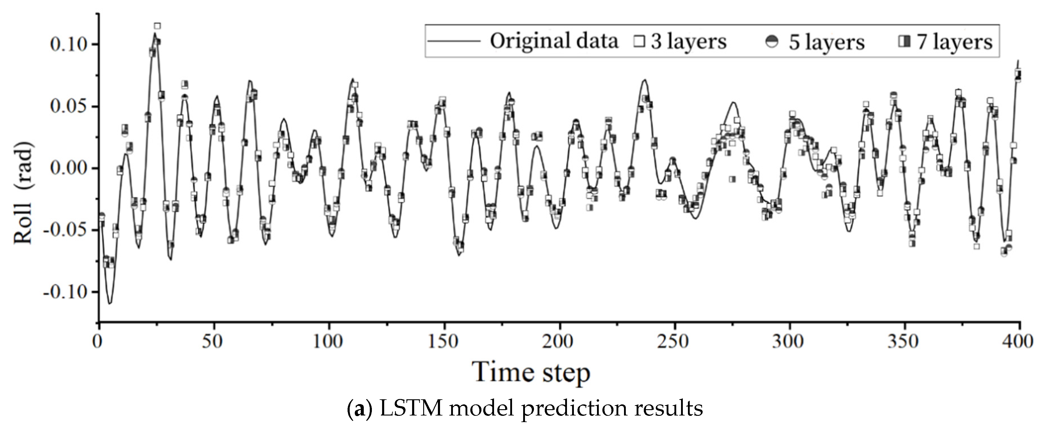
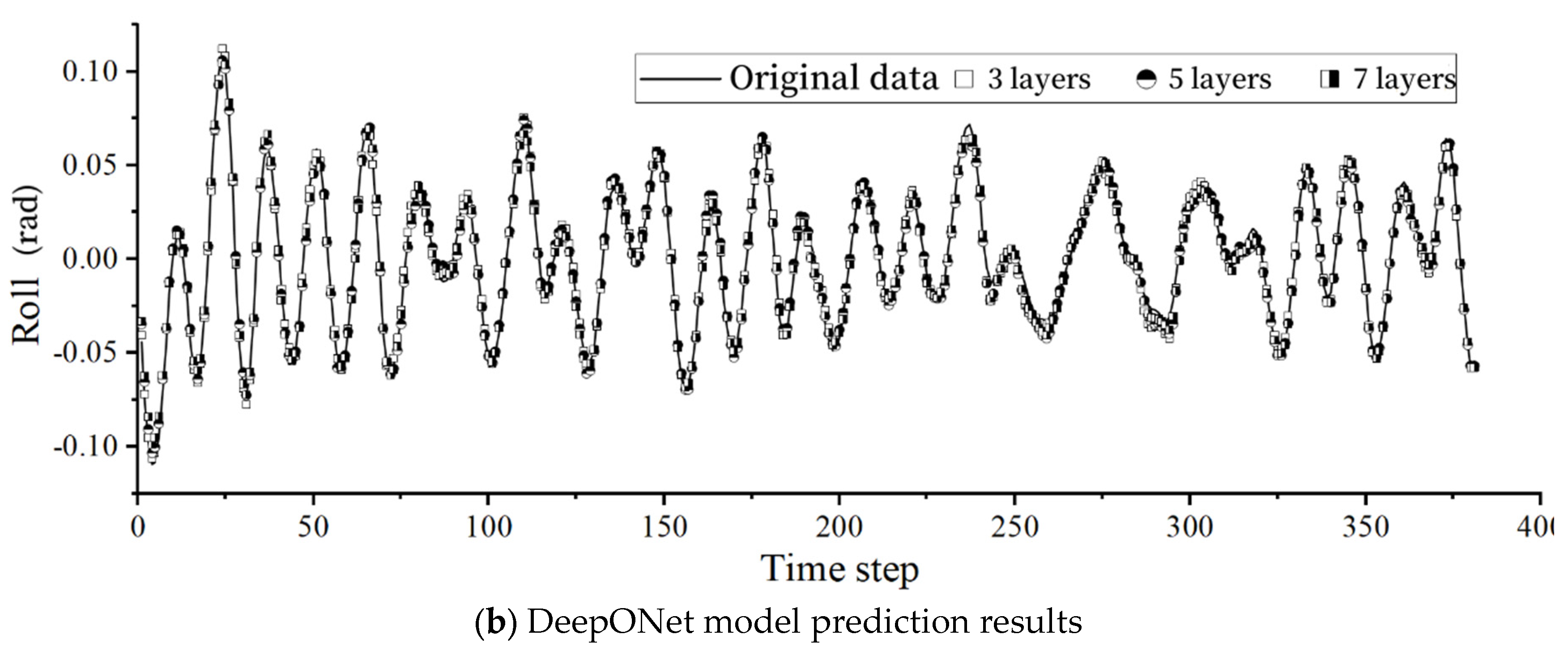
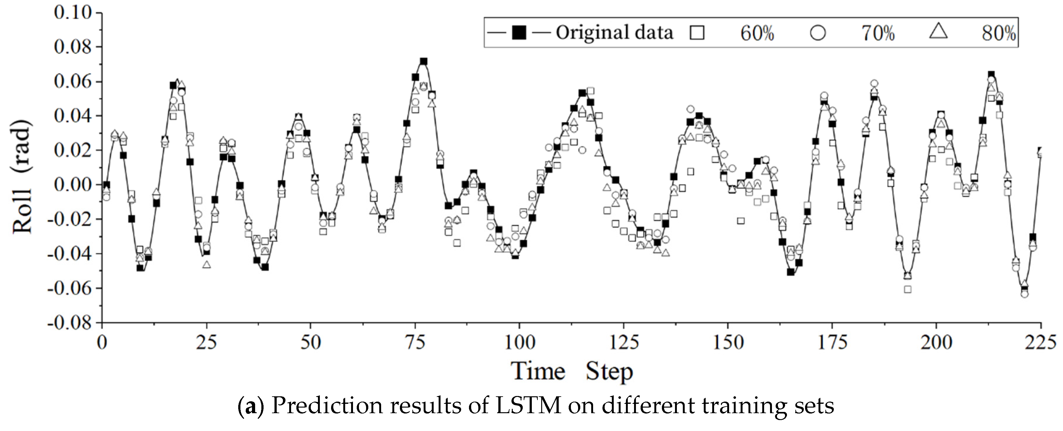
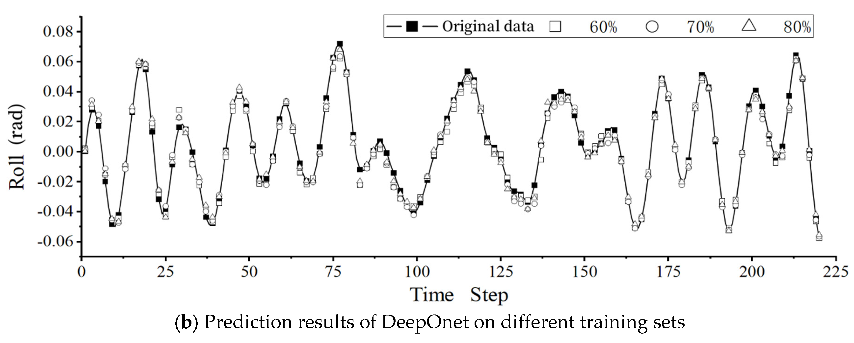
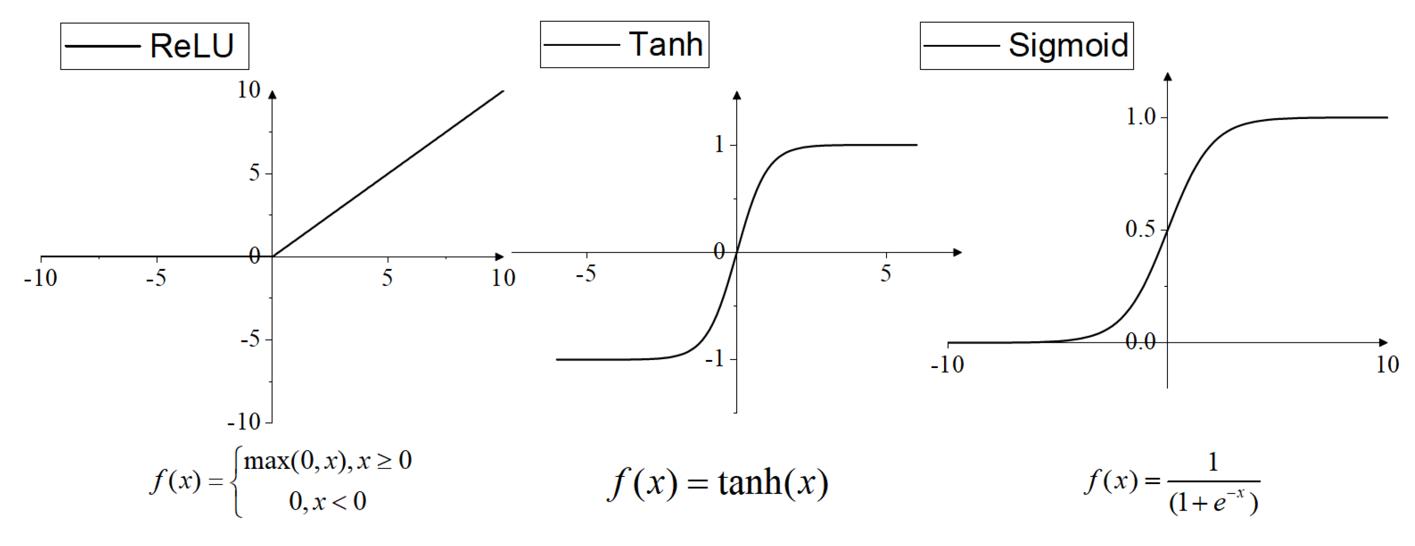
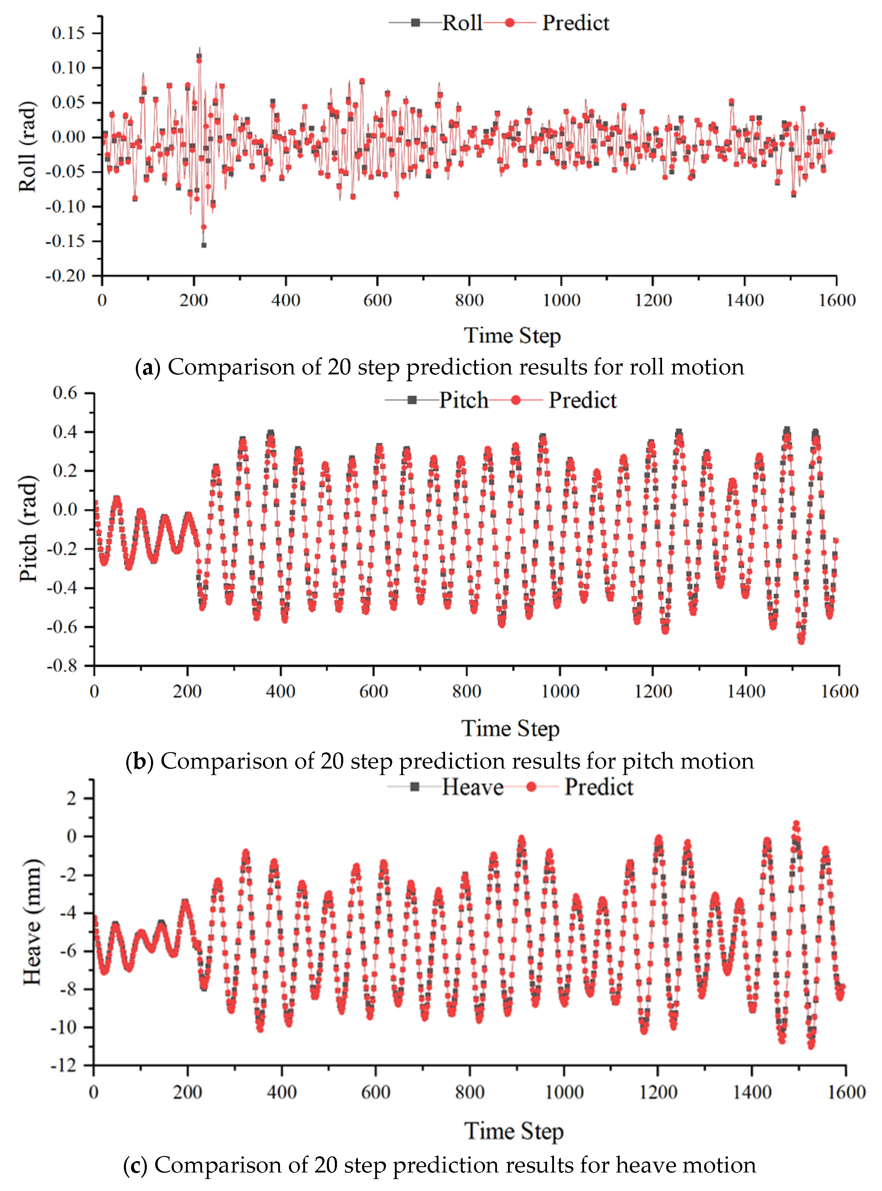
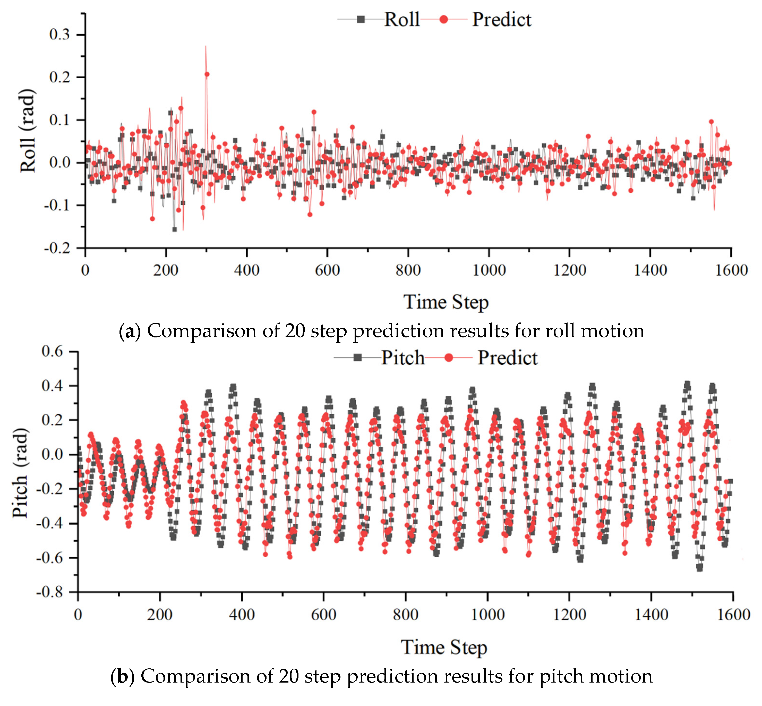
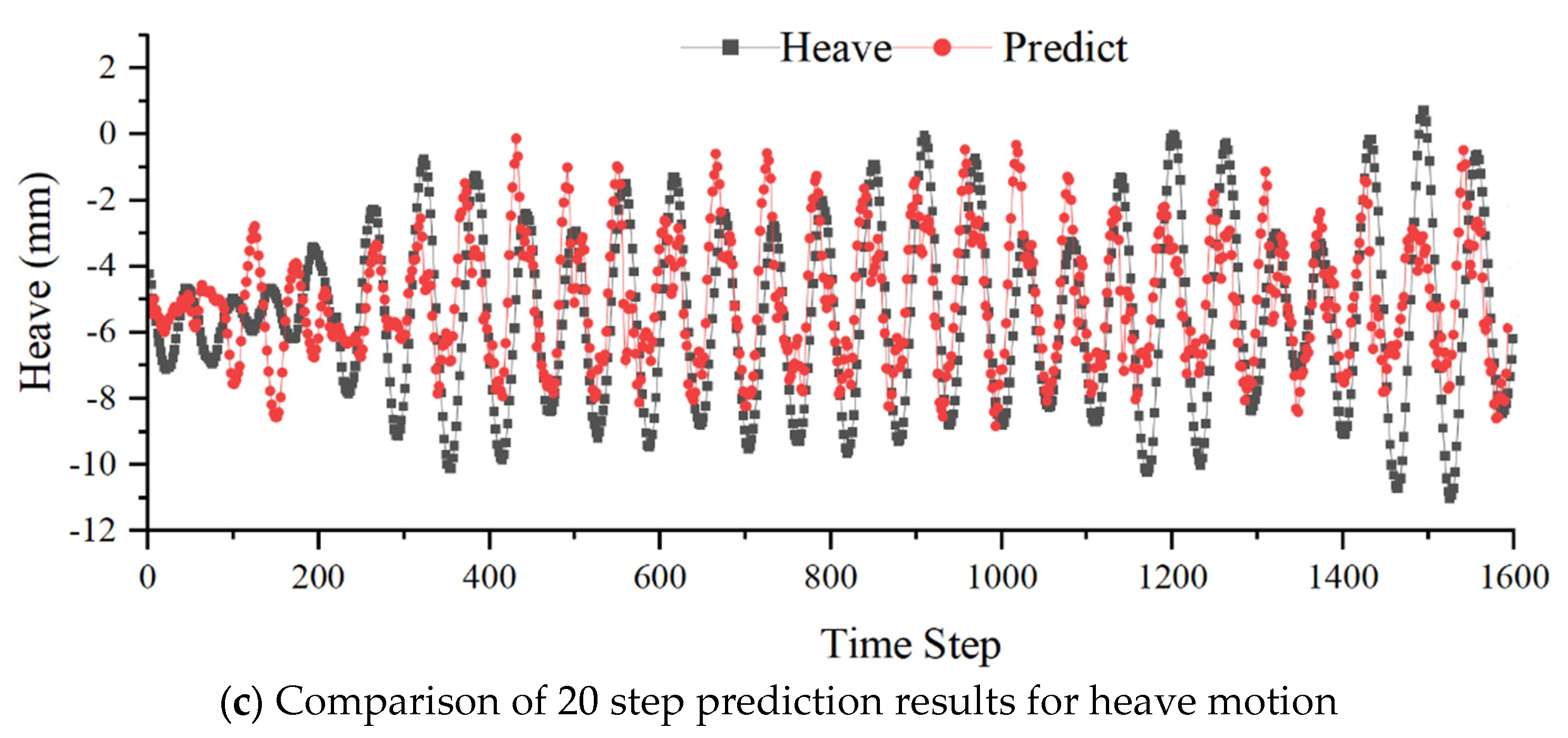
| Algorithm process: DeepOnet network |
|---|
|
Input: Window sliding is used to process the training set D1 and the test set D2. Hyperparameters are defined, including the number of layers and neurons in the two sub-networks (branch hidden layer and trunk hidden layer), the number of iterations, activation functions, learning rate, and loss function. |
|
Process: 1: Network initialization: Construct a list for hidden layers and initialize model parameters such as weights and biases. 2: Repeat; 3: For all D1; 4: Calculate the output y_branch based on the current weight parameters and the data passed into the branch network. 5: Calculate the output y_trunk based on the current weight parameters and the data passed into the trunk network. 6: Perform Einstein summation on the y_branch and y_trunk values in matrix form to obtain G(u)(y). 7: Calculate the gradient term of the output layer neurons. 8: Calculate the gradient term of the hidden layer neurons. 9: Calculate and update the connection weights. 10: End for. 11: Until the stopping condition is met. Output: The network model with the model parameters. |
| Parameter | unit | ship model 5512 | full ship size |
|---|---|---|---|
| Scale ratio | -- | 46.6 | 1 |
| Ship length (Lpp) | m | 3.048 | 142.04 |
| Beam (B) | m | 0.405 | 18.87 |
| Draft(T) | m | 0.132 | 6.15 |
| Block coefficient (CB) | -- | 0.506 | 0.506 |
| Fr | Uc(m/s) | H/λ=1/126 | AK | H(mm) | |
|---|---|---|---|---|---|
| 1 | 0.28 | 1.531 | 1/126 | 0.025 | 5.6 |
| 2 | 0.28 | 1.531 | 1/126 | 0.025 | 7.0 |
| 3 | 0.28 | 1.531 | 1/126 | 0.025 | 8.2 |
| 4 | 0.28 | 1.531 | 1/126 | 0.025 | 10.2 |
| Number of neurons | 80 | 100 | 120 | ||||
|---|---|---|---|---|---|---|---|
| Number of layers | DeepOnet | LSTM | DeepOnet | LSTM | DeepOnet | LSTM | |
| 3 | 1.526e-5 | 7.993e-5 | 9.166e-6 | 8.803e-5 | 1.605e-5 | 1.398e-4 | |
| 5 | 1.768e-5 | 1.049e-4 | 8.258e-6 | 1.044e-4 | 1.605e-5 | 1.261e-4 | |
| 7 | 1.517e-5 | 1.463e-4 | 9.660e-6 | 1.277e-4 | 6.431e-6 | 1.280e-4 | |
| Training set percentage | DeepOnet | LSTM | ||
|---|---|---|---|---|
| MSE | RMSE | MSE | RMSE | |
| 60% | 2.061e-5 | 4.5398e-3 | 1.731e-4 | 1.3157e-2 |
| 70% | 1.768e-5 | 4.2048e-3 | 8.803e-5 | 9.3820e-2 |
| 80% | 1.329e-5 | 3.6456e-3 | 5.243e-5 | 7.2410e-3 |
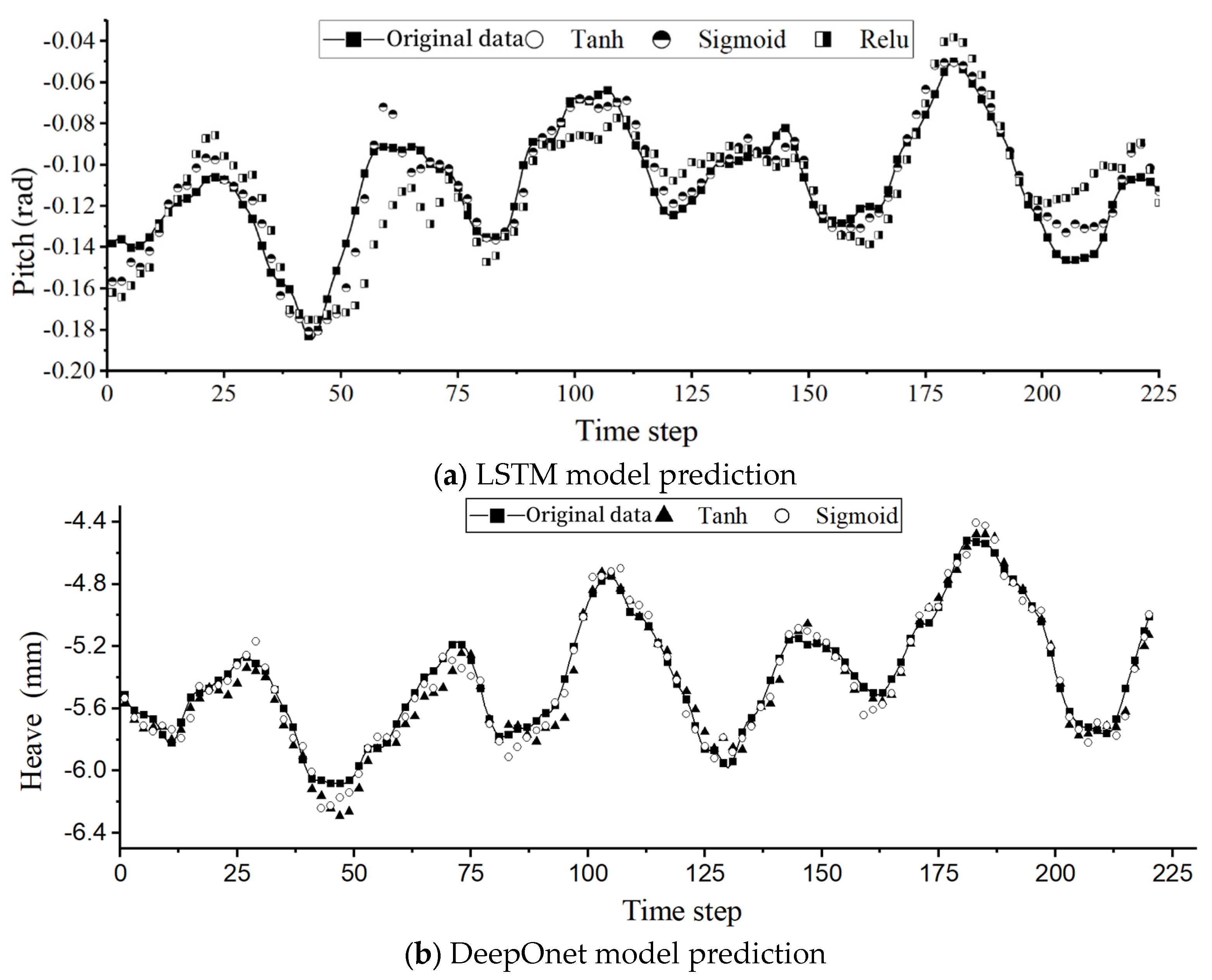
| MSE | Sigmoid | Tanh | ReLu | |||
|---|---|---|---|---|---|---|
| DeepOnet | LSTM | DeepOnet | LSTM | DeepOnet | LSTM | |
| Roll prediction | 8.64e-6 | 1.15e-4 | 8.25e-6 | 7.92e-5 | - | 4.69e-3 |
| Pitch prediction | 7.77e-4 | 1.19e-4 | 8.77e-6 | 6.52e-5 | - | 2.43e-4 |
| Heave prediction | 5.71e-3 | 1.28e-2 | 7.93e-3 | 7.33e-3 | - | 1.21e-2 |
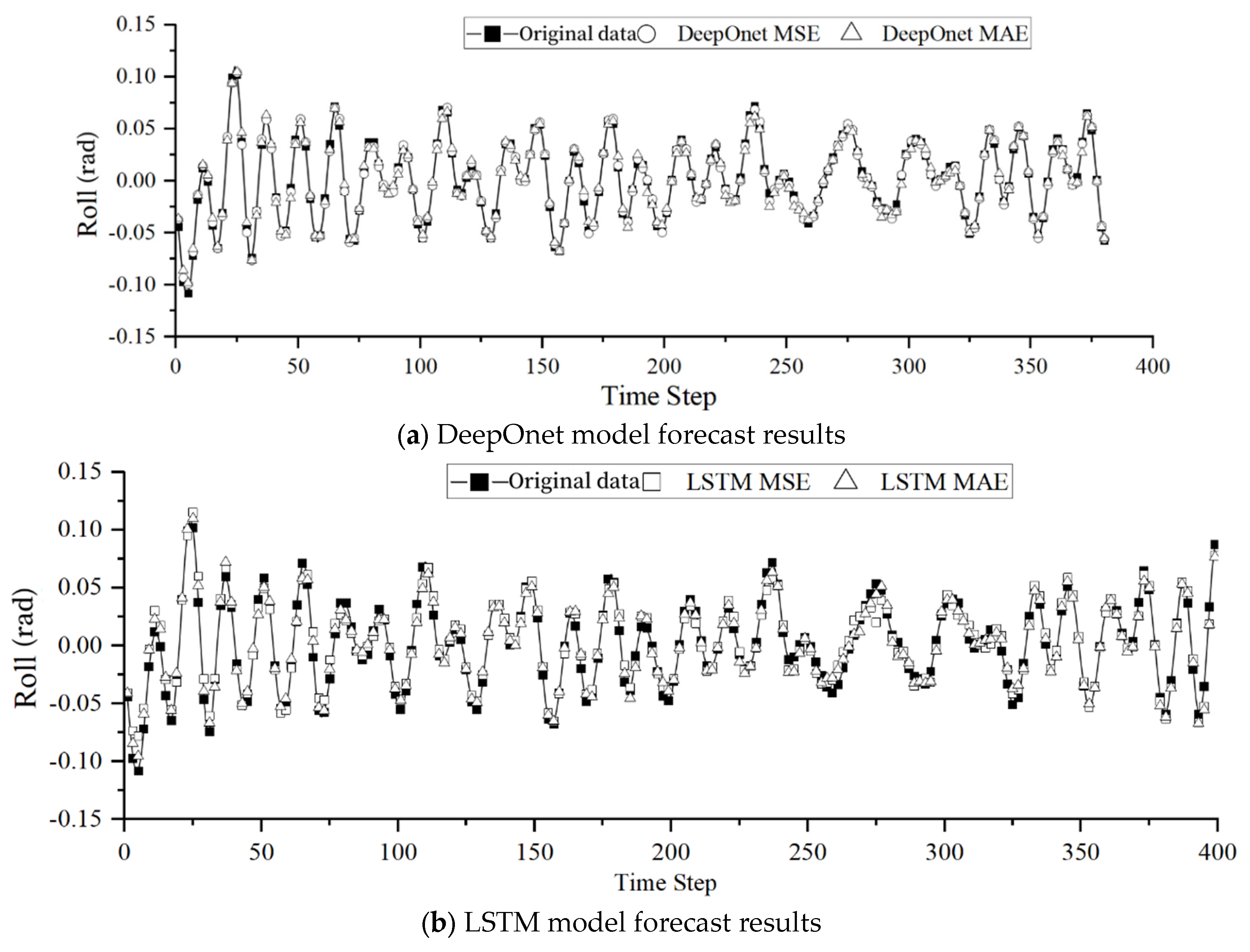
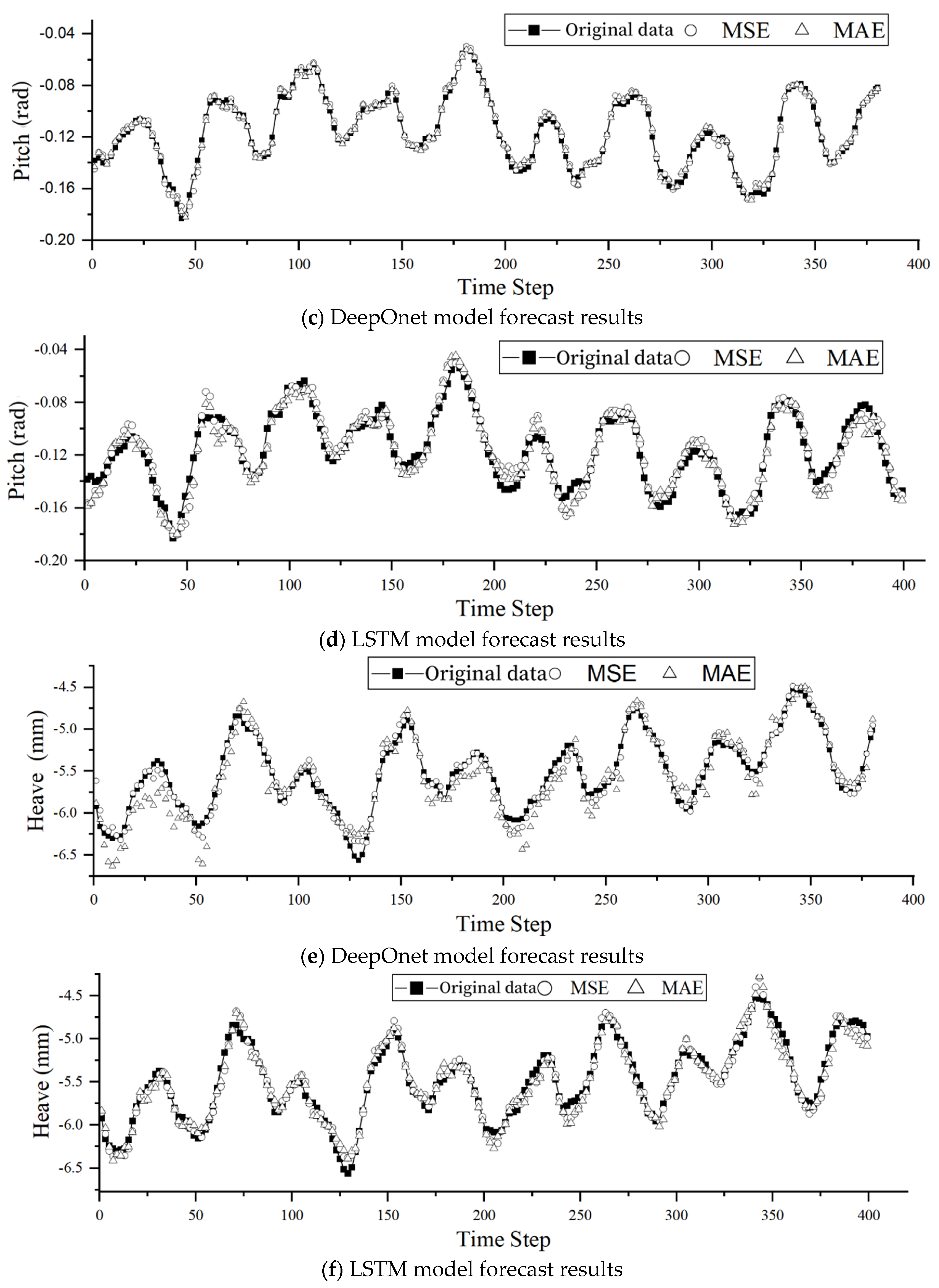
| Roll | Pitch | Heave | ||||
|---|---|---|---|---|---|---|
| DeepOnet | LSTM | DeepOnet | LSTM | DeepOnet | LSTM | |
| MSE | 8.25e-6 | 7.92e-5 | 8.77e-6 | 6.52e-5 | 7.93e-3 | 7.331e-3 |
| MAE | 3.29e-3 | 5.76e-3 | 2.61e-3 | 6.18e-3 | 1.44e-1 | 7.902e-3 |
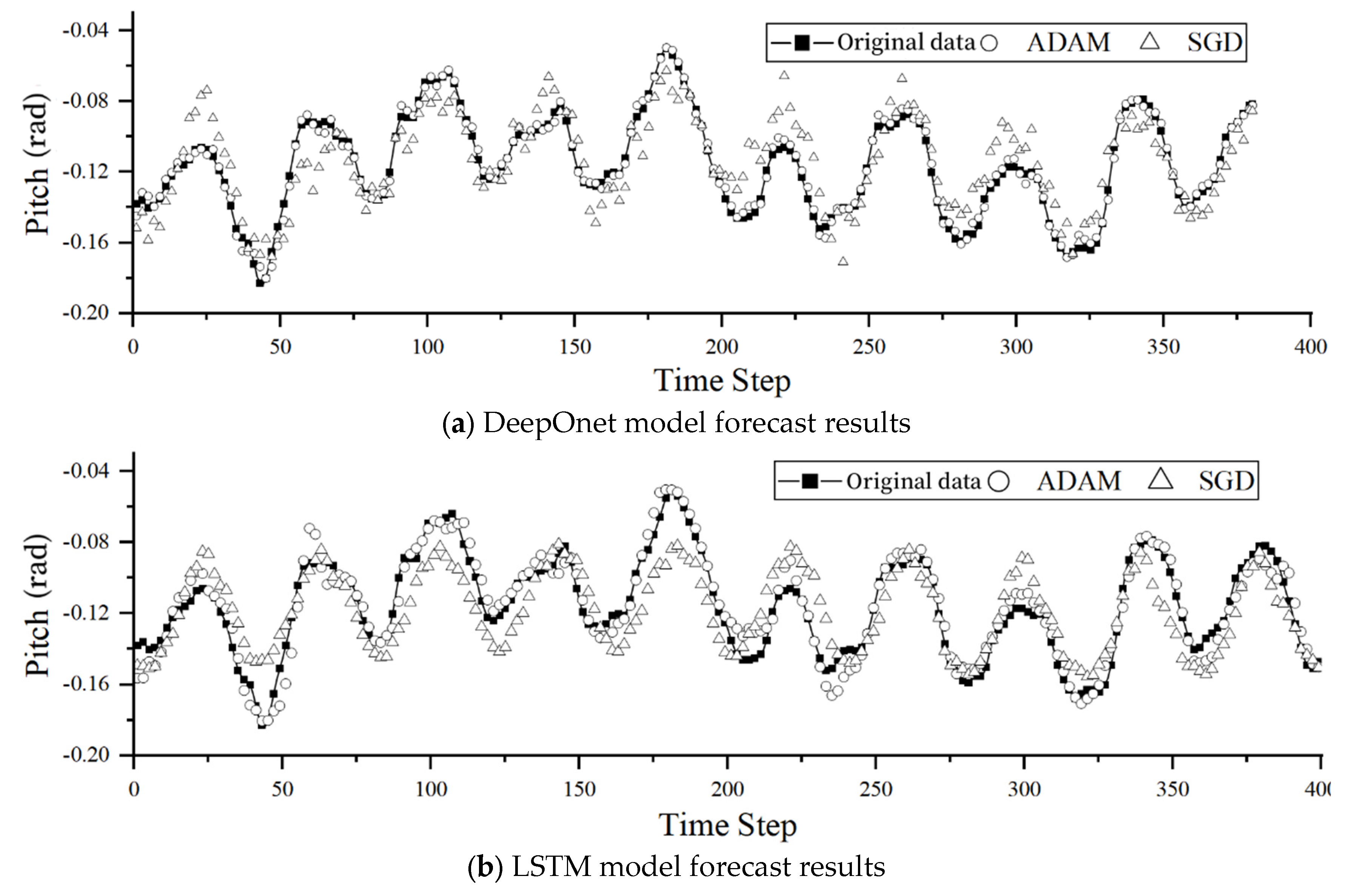
| Roll | Pitch | Heave | ||||
|---|---|---|---|---|---|---|
| DeepOnet | LSTM | DeepOnet | LSTM | DeepOnet | LSTM | |
| Adam | 8.25e-6 | 7.92e-5 | 8.77e-6 | 6.52e-5 | 7.93e-3 | 7.33e-3 |
| SGD | 1.32e-3 | 1.44e-3 | 2.58e-4 | 3.08e-4 | 7.29e-1 | 3.14e-2 |
| Prediction step size | Roll | Pitch | Heave |
|---|---|---|---|
| 1 | 3.472e-5 | 3.830e-4 | 8.680e-3 |
| 5 | 2.258e-5 | 1.893e-4 | 1.845e-2 |
| 10 | 2.083e-5 | 1.545e-4 | 1.822e-2 |
| 15 | 2.009e-5 | 1.459e-4 | 1.871e-2 |
| 20 | 2.022e-5 | 1.579e-3 | 1.889e-2 |
| Prediction step size | Roll | Pitch | Heave |
|---|---|---|---|
| 5 | 5.395e-4 | 1.782e-4 | 1.133e-1 |
| 10 | 6.675e-4 | 2.185e-4 | 1.211e-1 |
| 15 | 7.509e-4 | 3.488e-4 | 1.501e-1 |
| 20 | 8.490e-4 | 4.452e-4 | 2.290e-1 |
| Prediction step size | DeepOnet Roll | LSTM Roll | DeepOnet Pitch | LSTM Pitch | DeepOnet Heave | LSTM Heave |
|---|---|---|---|---|---|---|
| 5 | 2.258e-5 | 5.395e-4 | 1.893e-4 | 1.782e-4 | 1.845e-2 | 1.133e-1 |
| 10 | 2.083e-5 | 6.675e-4 | 1.545e-4 | 2.185e-4 | 1.822e-2 | 1.211e-1 |
| 15 | 2.009e-5 | 7.509e-4 | 1.459e-4 | 3.488e-4 | 1.871e-2 | 1.501e-1 |
| 20 | 2.022e-5 | 8.490e-4 | 1.579e-3 | 4.452e-4 | 1.889e-2 | 2.290e-1 |
Disclaimer/Publisher’s Note: The statements, opinions and data contained in all publications are solely those of the individual author(s) and contributor(s) and not of MDPI and/or the editor(s). MDPI and/or the editor(s) disclaim responsibility for any injury to people or property resulting from any ideas, methods, instructions or products referred to in the content. |
© 2024 by the authors. Licensee MDPI, Basel, Switzerland. This article is an open access article distributed under the terms and conditions of the Creative Commons Attribution (CC BY) license (https://creativecommons.org/licenses/by/4.0/).


