
You are currently viewing a beta version of our website. If you spot anything unusual, kindly let us know.
Preprint
Article
An Experimental Approach to Improve the Geometric Accuracy of Micro-features Fabricated by Stereolithography (SLA)
Altmetrics
Downloads
184
Views
68
Comments
0
A peer-reviewed article of this preprint also exists.


This version is not peer-reviewed
Abstract
In this paper, we present an experimental procedure to enhance the dimensional accuracy of fabrication via Stereolithography (SLA) of features at the micro-scale. Using a custom benchmark part, deviations in feature dimensions (micro-pores diameters and depths) were detected and measured by confocal microscopy. Samples characterization and experimental observations allowed the identification of inaccuracy sources, mainly due to the laser beam scanning strategy and to the incomplete removal of uncured liquid resin in post-processing (i.e., IPA washing). As a technology baseline, the measured dimensional errors on pores diameters were up to -46%. A compensation method of the nominal laser spot diameter (85m) was defined and implemented resulting in relevant improvements in dimensional accuracy of 9.8% and 11.3% on full-open pores diameter and depth, respectively. Further investigation was performed on a customized test part to adjust the calibration procedure. The measurements revealed that the estimate of the laser beam spot size is 968m. Measurements on micro-pores having different sizes revealed that a constant compensation parameter (i.e., C=85, 96, 120m) is not fully effective at the micro-scale, where average errors still remain at -24%, -18.8%, and -16% for compensations equals to 85, 96 and 120m, respectively. A further experimental campaign allowed the identification of an effective nonlinear compensation law where the compensation parameter depends on the micro-feature size C= f (D). Results show a sharp improvement in dimensional accuracy on micro-pore fabrication, with errors consistently below +8.2%. The proposed compensation method can be extended for the fabrication of any micro-features without restrictions on the specific technology implementation. Concerning the inaccuracy introduced by the laser path, experimentation with a customized part allowed the optimization of the part orientation to reduce the errors and their differences along the X and Y machine axes.
Keywords:
Subject: Engineering - Industrial and Manufacturing Engineering
1. Introduction
Among Additive Manufacturing (AM) technologies, Stereolithography (SLA) is largely used to fabricate parts with intricate 3D geometry, and very accurate features, due to its performance, high speed, resolution, high precision, smooth finishing, low waste, and affordability of polymers, composites and ceramics materials, with a fully-digitalized process [1]. SLA belongs to the family of VAT Photo Polymerization (VPP) technologies, and it exploits liquid photopolymers, which are polymerized by a laser beam spot (LBS) that scans and UV-cures the material, layer by layer.
The SLA process with its variants (top-down and bottom-up exposure) is, among other applications, successfully used to fabricate regular/high-ordered porous 3D microstructures [2,3]. Figure 1 shows an inverse opal, a face-centered cubic structure (FCC), fabricated via bottom-up SLA.
Several studies were conducted with different objectives: development of advanced applications, process parameters optimization, investigation of new materials performance and processability, addressing technology issues and process sustainability, conceiving innovative process chains, etc. [4,5,6,7,8]. Remarkable achievements were obtained by investigating SLA process parameters aiming at identifying their effects on the 3D-printed part quality: dimensional accuracy, surface finishing, mechanical properties, defects occurrence, etc. Sabbah A. et al. [9] found a negligible impact of the layer thickness (LT) on surface finishing, while it strongly affects the dimensional accuracy of 3D-printed parts. The minimum layer thickness of 25μm resulted in higher precision. Cotabarren, I. et al., confirmed that layer thickness is a critical parameter for part accuracy; measurement deviation was reduced by about 90% when this parameter was reduced from 100 to 25μm [10].
Arnold C. et al. [11] concluded that the surface roughness of 3D-printed parts is firmly dependent on the model orientation in the build volume. The best results were obtained with a 0-degree part orientation (surface lies horizontally on the build platform) with measured values of Ra=1.15±0.47 μm along the X-axis and Ra=0.90±0.33 μm along the Y-axis. Other similar studies confirmed these results [12]. Shanmugasundaram S. et al. investigated the effects of printing orientation on the part’s mechanical properties, and no significant anisotropy was detected thanks to UV-curing post-processing [13]. Hada, T. et al. found that the highest dimensional accuracy is achieved by orienting the part with a 45-degree angle on the build platform, followed by a 90-degree orientation. The worst orientation is the 0-degree with the part parallel to the build platform [14]. These results were also confirmed by other studies [15,16].
As it can be noticed, several works focused on the influence of process parameters on the quality of 3D-printed parts, but there is a lack of research studies on the effects of the laser-scanning path and post-processing operations on the feature accuracy, especially at the micro-scale.
An original approach was implemented by Wen C. et al. [17], who investigated the geometric accuracy of microstructures of a Projected SLA, also known as Digital Light Processing (DLP) technology. They identified a compensation method of inaccuracy introduced by the light power intensity distribution. The proposed solution is based on structure optimization using a compensation parameter derived by the simulation results. The micro-features design (circles, squares, and triangles) is modified in dimension and shape to increase the dimensional accuracy. This compensation strategy allows the achievement of a mean error reduction from 21-23% down to 1.6-4.8%.
In the present study, the dimensional accuracy of the manufacturing of micro- features and structures via SLA technology was investigated and an approach for inaccuracy compensation has been conceived and tested. It is an extension of a previous preliminary study [18]. The laser beam spot and laser path were experimentally analyzed and inaccuracy sources were identified and addressed. The investigation revealed that a considerable part of the geometrical error was related to the laser path. However, by decreasing the feature’s size other phenomena become more important. Therefore, the study focused on two main aspects: i) laser path improvement; ii) identification of a compensation factor that considers both an estimation of laser beam spot diameter and other phenomena that affect the geometrical accuracy. The technology limitation was evaluated, and effective solutions were proposed, thus increasing the SLA capability and accuracy of the fabrication of micro-features at the micro-scale.
2. Materials and Methods
Micro-pore features are the fundamental component of all porous materials, as a single feature (1D), or replicated in a surface texturing (2D planar or freeform patterns) or in a volume (3D). In the latter case, if the pores are regularly distributed along the three directions in a pattern, the resulting structures are lattices. All these cases are characterized by a single pore or a single cell, including pores and fractions of pores. For this reason, the proposed approach investigates the fabrication of a single pore and its accuracy. The investigation on the fabrication by SLA of porous micro-features was performed by designing a sample with Full-open pores (FOP), thus hemispherical cavities, with variable diameters from 1 mm (1-A) down to 0.5 mm (6-A) with a step of 100 μm (Figure 2) and reported in Table 1. Figure 2 also shows the SLA fabricated samples before the detachment from the base and supports.
Each geometry was realized in three samples with the parameters reported in Table 2. The equipment adopted for fabricating the samples is a Formlabs Form 3 (Formlabs Inc., USA), having a build volume of 145×145×185 mm3, equipped with a class 1 violet laser emitting at a wavelength of 405nm with a nominal laser beam spot diameter DLS of 85 μm and a power of 250 mW. The positioning resolution on the x-y plane is 25 μm, while the z-axis resolution can be set from 200 to 25 μm (layer thickness). Samples were designed with the 3D CAD Solidworks 2017 (Solidworks Corp., Dassault Systèmes, USA), exported to Stereo Lithography interface (STL) format, and then imported into the Formlabs slicing software Preform v.3.32.0. In this software environment, parts were oriented, and all the process parameters were chosen according to the database supplied by the machine manufacturer and to previous studies [6,12,19]. The surface with micro-pore features was oriented horizontally, thus parallel to the build platform, which guarantees a higher surface finishing [12,19]. The process parameters are reported in Table 2.s
Samples were fabricated in Formlabs Clear V04 photopolymer resin, identified by the manufacturer’s code RS-F2-GPCL-04 [20]. After the SLA processing, parts were removed from the build platform and washed for 20 minutes into high-purity 99% isopropyl alcohol (IPA) and 5 minutes with ultrasound washing. Samples were acquired with an optical profilometer Sensofar S-Neox (Sensofar group, Barcellona, Spain), set with a Focus Variation acquisition method, using an objective EPI 10X with numerical aperture NA of 0.30 and a pixel resolution of 1.29 µm. Acquired images were processed by means of algorithms of the ImageJ software (National Institutes of Health NIH, USA) version 1.54g. The images were processed using a “threshold” (Figure 3a) and a “analyze particles” (Figure 3b) algorithms. This image processing procedure automatically gives several parameters regarding the shape (such as roundness, circularity, and solidity indexes) and size (such as area, perimeter, width, and height) of the region of interest (i.e., cavity or particle). The average diameter of each pore is calculated by the measured area using the formula: Diameter = .
2.1. Effect of the Laser Scanning Path
In order to investigate the effects of the laser beam path generation on the final part accuracy, a specific component, referred to as Laser Path Evaluation Part (LPEP), was designed with both simple holes and protrusions. The CAD model was then imported into the Formlabs Preform slicing software and the laser path was generated. The LPEP was oriented flat on the build platform (horizontal, Figure 4a) and preprocessed with the Preform algorithms to generate base, supports, slicing, and laser beam paths (Figure 4b). Figure 4 reports the slicing and laser beam paths of circular and squared holes (Figure 4c,d) and protrusions (Figure 4e,f). Looking at the generic slice of the region with holes, it can be easily recognized that the laser beam path starts exactly on the hole edge, and it proceeds with a double-contour path of the 2D-slice geometry. This step of the layer curing strategy is also referred as the “perimeter” step. The bulk material, which is the external region of the hole, is then UV-cured by a rectilinear infill with linear parallel laser beam paths and a distance between them likely equal (or slightly smaller) to the nominal laser spot diameter. The same observations can be done looking at the protrusion features. The laser beam path contours the protrusion edges towards the material side with two contours or perimeters, the first on the protrusion edge and the second with an offset from the first. The internal region of the protrusion is filled with a rectilinear path oriented according to the part orientation (see Figure 4).
The hypothesis is the following. If the circular laser spot, having a diameter of DLS, is centered on the line path, then all the edges of the slices, no matter if hollowed or protrusions, will be affected by an over-polymerization equal to the laser spot radius on each side or edge. This will result in smaller holes and larger protrusions than nominal ones. Each laser spot polymerization of the current layer has a volume that can be approximated to VLS=DLS*LT, and the over-polymerized volume equal to DLS*LT/2 will occur along the edges. Of course, at the meso and macro-scale, this inaccuracy is not relevant since it is a small percentage of the nominal dimensions, but it is very important at the micro-scale, where nominal dimensions are of the same order as the laser beam spot diameter. The hypothesis is schematized in Figure 4g,h).
If this hypothesis is confirmed, then inaccuracy occurs due to the missing compensation of the laser spot radius in the laser path generation algorithm, and a compensation method can be developed and applied. Since it is not possible to modify the laser path in the Preform slicing software, an effective strategy consists in applying an offset volume to the 3D models, i.e., as a general rule, by increasing the cavities and by reducing protrusions. The offset value should be carefully identified. In the simple case of hemispherical pore micro-features, the compensation to the model pore diameter is DP =DNP+C, where DNP is the nominal pore diameter, and C is the compensation parameter.
In order to investigate other sources of inaccuracy, Section 3.1 presents a preliminary test considering the designed FOP pore micro-features without and with compensation. Further investigations were executed to achieve an empirical esteem of the parameter C. Results are presented in Section 3.2. The effects of the constant compensation strategy with different values of the compensation parameter are discussed in Section 3.3. Finally, a deep analysis of the experimental data suggested a calibration procedure based on a variable compensation parameter taking into account the dependency of C from the feature size (i.e., micro-pore diameter). The procedure and results are presented in Section 3.4.
3. Results and Discussion
3.1. Preliminary Test: Measurements of Full-Open Micro-Pores (FOP)
Preliminary tests are performed by 3D printing the designed FOP micro-features without and with the compensation C, defined as equal to the nominal laser beam spot diameter DLS=85μm. The diameters and depths measurements of micro-pores are reported in Table 3 with their mean values and standard deviations; the same data are shown in Figure 5.
The average error on pore diameters spans between -92 and -135 µm, and it is consistent (in value and sign) with the hypothesis of missing compensation of the laser beam spot radius on contours. Further confirmation arises from the measured diameter considering a compensation C= 85µm, increasing the pore dimension accordingly. In this latter case, the reduced error spans between -25 and -75 µm. It is also possible to observe that the error increases when the pore diameter decreases. This behavior can be attributed to the adhesion of the uncured liquid resin on the solid surface due to surface tension, whose effect increases as dimensions decrease and becomes evident for cavities with sub-millimetric diameters. Thus, the IPA washing aimed at removing uncured resin residuals is less effective on pores at the micro-scale, preventing the fabrication of micro-cavities below a threshold size.
The depth of the pores is affected by an average error that spans between -35 and -179µm, which is reduced when the compensation is adopted, varying between 3 and -103µm. The compensation has a beneficial influence on the depth error because it enlarges the cavity, producing two effects: it dampens the cutoff of the geometry slicing and reduces the resin adhesion effect.
3.2. Esteeme of the Compensation Parameter
The preliminary test reveals that the error in diameter is not fully compensated by adopting C equal to the nominal laser spot diameter, also at a millimetric scale.
An assessment of C has been attempted by printing and measuring the part shown in Figure 6, which presents four repetitions of six squared thin wall features. The wall thicknesses vary in the following sequence: 0.05, 0.1, 0.15, 0.2, 0.25, and 0.17 mm.
Since slicing always has two paths on the edges of each thin wall, a feature with a wall thickness equal to two times the laser beam spot nominal diameter (170μm) was added at the end of the pattern. Figure 6a shows the drawing of the proposed part for the correction factor estimation. Samples were fabricated according to the described conditions (Section 2) and parameters (Table 1). A sample of the part is shown in Figure 6b,c.
The difference between the nominal and the measured wall thickness returns an estimate of how much the geometrical edge must be moved (offset) to achieve the complete compensation. The measurements are reported in Table 4 with the estimated value of C.
The C value ranges between 88 and 102 µm, with an average value of 93 µm and a standard deviation of 8 µm. It must be observed that the average value tends to be greater than the nominal diameter of the laser spot (85 µm), with a growing trend when the wall thickness is thinner. This latter effect seems to be related to the step-over of the two on-edge laser paths (squares from 1 to 3), which increases when the wall thickness decreases. The high values of standard deviations are attributed to the different infill of the wall when the thickness increases at higher values (squared walls 4, 5, and 6). In fact, in these cases, when the wall thickness is higher than the laser beam spot diameter, the infill strategy is a rectilinear scan oriented along the machine y-axis. With this evidence (Figure 7), all walls oriented along the x-axis are filled with a pattern of parallel lines orthogonal to the wall edge. In contrast, all walls oriented along the y-axis are filled with additional lines along the wall edge.
Therefore, this different infill strategy determines different UV-curing for the same walls with related variable thickness, thus higher values of standard deviations in measurements. Figure 8 reports the graph of measurement of thin wall thicknesses and the estimated compensation parameter C. Nominal values of thin walls are represented by the slanted black dashed line. All deviations from this line are fabrication errors to be quantified. The values of the actual thin wall thicknesses along x- and y-axis are depicted with blue and green solid lines, respectively.
All measured thicknesses are higher than the nominal ones. The average wall thicknesses are depicted with a gray dashed line. As can be seen in the figure, wall thicknesses along the x-direction (blue line) are greater than those along the y-axis (green line), but the difference between them decreases beyond the threshold value of t*=150 μm. The differences between measured and nominal values are reported with an orange line.
As observed before, the estimated C is almost stable to about 100 μm up to the t*, and it decreases to 82-88 μm with thicknesses higher than t*. Indeed, up to t*, the infill is missing along the y-direction, while it is always present along the x-direction. The infill strategy significantly affects wall thickness accuracy, producing a different wall thickness depending on the wall orientation and nominal thickness, as shown in Figure 8.
The error on the thin wall thickness is 74±4.5 µm and 112±11.9 µm along the y- and x-axis, respectively. The graph in Figure 8 shows that the error on the wall thickness along the x-axis (blue line) is slightly reduced when its value is greater than 170μm, two times the nominal laser spot diameter. These data suggest that the current infill strategy produces geometrical anisotropy on features. Therefore, the part orientation on the XY plane affects the geometrical accuracy at the micro-scale. A different infill strategy (i.e., offset of the external perimeter) can improve the geometrical accuracy and reduce the anisotropy. More easily, an effective strategy to compensate for this anisotropy is an optimized orientation of the part on the build platform. Since the on-use machine allows only y-axis linear infill, an effective solution is a 45-degree orientation of the part on the XY plane (build platform).
Figure 9 shows the results obtained with the 45-degree orientation. The plot of the thin-wall measurements is depicted in Figure 9a, while a picture of the confocal acquisition is reported in Figure 9d. This part orientation (Figure 9b), generates linear infill patterns (red lines in Figure 9c) inside the wall thickness, which results in a sharply reduced anisotropy: same thickness (and error) along both the x- and y-axis. In fact, as it can be seen in Figure 9a, the graph lines (green and blue) of measurements along the two axes are almost superimposed but still exhibit an error due to the missing compensation. Four samples were 3D-printed at different positions on the build platform. The measurements and statistical values are reported in Table 5.
3.3. Constant Compensation Strategy
Since variability in the esteem of C has been found, the constant model compensations strategy was applied to the micro-pore diameters considering three levels of compensation:
- C=+85 μm, is equal to the nominal laser spot diameter;
- C=+96 μm, is the value obtained with the calibration tests;
- C=+120 μm, value identified as the average error on diameter obtained in the preliminary tests when the compensation of +85μm was applied.
Figure 10 shows the effects of the constant compensation strategy compared with the curve obtained without compensation.
As can be seen from the figure, the constant compensations – the same value of the parameter C for all pores – are not fully effective, especially at the small scale (diameters below 1,2 mm), where the error dramatically increases. The smaller the micro-pore, the higher compensation is required. Furthermore, the value of C=120μm produces an overcompensation (positive errors) for feature diameters higher than 1.0 mm, and similar results are obtained with C=85μm for feature diameters higher than 1.6 mm.
From these results, it can be concluded that inaccuracy related to the laser spot diameter is the most important and can be effectively compensated for pore dimensions down to about 1.2 mm. When the pore diameter gets smaller and smaller, other phenomena become more dominant, and the constant compensation is no longer effective. However, a strategy of variable compensation based on the feature size and the error trend can be investigated in order to empirically compensate all the sources of inaccuracy.
3.4. Variable Compensation Strategy
The results presented in the previous section clearly suggest that a nonlinear compensation law could be more effective than a constant or a linear compensation strategy as the pore dimension decreases to take into account phenomena typically arising at the microscale, such as adhesion and surface tension.
The nonlinear compensation law can be derived by processing the experimental data set. Its identification was performed by following three steps:
- Plot of all measurements of features on samples (i.e., FOP pore diameters), with and without compensations;
- Identification by polynomial regression of a mathematical relationship between actual and nominal values of the meso- and micro-feature size;
- Solving the equation obtained in the previous step, thus the value of the compensation parameter can be derived as a function of the feature size C = f(D) (i.e., pore diameter).
According to this procedure, data of nominal and actual diameters were plotted and analyzed. The polynomial model order for data identification was chosen as a trade-off between the mathematical complexity and the statistical confidence (coefficient of determination R2) in the model’s data prediction. A second-order polynomial interpolation model (three parameters) was identified by the Microsoft Excel regression algorithm, resulting in a value of R2=0.9954, which was considered satisfactory for the objective of the work. The model equations (explicit and implicit forms) are given by:
where y is the actual (measured) diameter, x is the related nominal diameter, and (a, b, c) are the parameters of the 2nd-order polynomial regression model. The values of the model parameters are: a = -0.0001; b = 1.3641; c = -385.77. The equation (1) was solved to obtain the nominal (compensated) values (x) of diameters that give the desired (y) values. Finally, the values of the required compensation parameter C are calculated as the difference between the measured and the compensated values of the pore diameters:
The model prediction of diameters and the related compensations were plotted on an extended and denser range of the nominal diameters (Figure 12). The curve of the variable compensation parameter (yellow line) reveals that for bigger features (diameters bigger than 1.2 mm), the compensation has values close to the constant nominal compensation and does not vary significantly. For this reason, at the meso scale, a variable compensation is not required, and a constant compensation strategy can be adopted. Therefore, it can be concluded that a discontinuity occurs in the compensation law: variable compensation at the micro-scale, down to D’=1200μm and a constant compensation law beyond this threshold.
Four samples were 3D-printed at different positions on the build platform in order to explore the possible effects of this parameter on data dispersion and part accuracy (Figure 14). Each sample reports a pattern of three sequences of full-open pores with eight target diameters in the range 500-2000μm. The compensation parameter for diameters higher than 1200μm was set to 96μm, thus the estimated value of the laser spot diameter obtained in Section 3.3. The drawing of the samples is depicted in Figure 13, and the nominal value of diameters and compensation parameters are reported in Table 6.
The error percentages calculated on sample measurements with their dispersions are reported in Figure 15. The curve of variable compensation (blue line) reveals a sharp improvement in accuracy with errors below 8.2%. The best sample error (yellow curve) is always below 4.4%. A slight overcompensation occurs at the micro-scale (below 900μm). Furthermore, a constant compensation strategy beyond D=1200μm is confirmed to be the best choice.
Table 7 reports mean errors and standard deviations without compensation and with constant and variable compensation.
As can be noticed, the absolute and percentage errors progressively decreased from no compensation to variable compensation. Also data dispersion has been improved. These results demonstrate that a compensation strategy increases the accuracy of technology, especially at the micro level. Furthermore, a variable compensation method based on the feature dimension is successful since it allows further improvement compared to the constant compensation strategy.
4. Conclusions
In this study, an SLA process was analyzed in terms of dimensional accuracy addressing micro-feature fabrication by investigating the effects of inaccuracy due to scanning paths, laser spot compensation, and post-processing operations. This analysis brought up that the accuracy of the fabrication can be improved introducing a compensation factor for the laser spot diameter and for the laser scanning path generation. The first attempt promoted in this work was a constant compensation applied to the part 3D model based on the nominal laser beam diameter, which is 85μm for the used equipment. This method increased the accuracy up to 20% and 30% on micro-pore diameters and depths, respectively. A benchmark test part was then conceived and used to estimate the actual compensation parameter, estimated as 96±8 μm, with a deviation of +12.9% from the nominal value.
The constant compensation strategy succeeds at the meso scale (i.e., D>1200μm), but fails at the micro-scale (i.e., D=500÷1200μm), where the dimensional accuracy remains low: error percentage up to 24.8%. This not negligible error is attributed to uncured resin, which remains trapped in the micro-pores where the removal by IPA washing is less effective. The analysis of the experimental data revealed that a variable (nonlinear) compensation method with the compensation parameter as a function of the micro-feature size (i.e., micropore diameter) is more suitable and effective. The variable compensation law for micro-pores was derived by the analysis of the experimental data obtained in the previous steps. A second-order polynomial regression law was used to obtain the nonlinear compensation with confidence of R2=0.9954. According to this new strategy, a final experimental campaign was performed. Measurements of samples showed a relevant increase in accuracy on micro-pore diameter, with an error percentage below 8.2%.
Regarding the technology, this study suggests improvements of the path generation strategy by compensating the actual laser spot diameter and optimizing the infill strategy.
This study focused on simple spherical micro-porous, and it did not consider complex geometries, which can require a challenging assessment to identify the correct compensation laws along the three axes. Other aspects to be investigated are the role and effectiveness of the IPA-washing post-processing, surface tension, and photopolymer viscosity in eliminating the trapped liquid resin into micro-pores and porous structures.
Author Contributions
Authors F.M. and V.B. contributed equally. Conceptualization, methodology, software, validation, writing—original draft preparation, F.M. and V.B.; writing—review and editing, V.B., F.M. and I.F.; supervision, I.F.. All authors have read and agreed to the published version of the manuscript.
Funding
This work was partially supported by the European Union under the Italian National Recovery and Resilience Plan (NRRP) of NextGenerationEU, a partnership on “Telecommunications of the Future” (PE00000001 - RESTART) and on “Made in Italy Circular and Sustainable” (PE00000004-MICS). This manuscript reflects only the authors’ views and opinions, neither the European Union nor the European Commission can be considered responsible for them.
Conflicts of Interest
The authors declare no conflict of interest.
References
- Kafle, Abishek, et al. “3D/4D Printing of polymers: Fused deposition modelling (FDM), selective laser sintering (SLS), and stereolithography (SLA).” Polymers 13.18 (2021): 3101.
- Bártolo, P. J., ed. Stereolithography: materials, processes and applications. Springer Science & Business Media, 2011.
- Zhang, F., et al. “The recent development of vat photopolymerization: A review.” Additive Manufacturing 48 (2021): 102423.
- Maines, Erin M., et al. “Sustainable advances in SLA/DLP 3D printing materials and processes.” Green Chemistry 23.18 (2021): 6863-6897.
- Muldoon K.et al.”High Precision 3D Printing for Micro to Nano Scale Biomedical and Electronic Devices.” Micromachines 13.4 (2022): 642.
- Basile V. et al. “Analysis and Modeling of Defects in Unsupported Overhanging Features in Micro-Stereolithography.” Proc. of ASME 2016 IDETC-CIE. Vol. 4. Charlotte, NC, USA. August 21–24, 2016. V004T08A020. 21 August.
- Schmidleithner, Christina, and Deepak M. Kalaskar. “Stereolithography.” IntechOpen, 2018. 1-22.
- Huang, Jigang, Qin Qin, and Jie Wang. “A review of stereolithography: Processes and systems.” Processes 8.9 (2020): 1138.
- Sabbah A. et al. Impact of layer thickness and storage time on the properties of 3d-printed dental dies. Materials 14.3(2021): 509.
- Cotabarren, Ivana, et al. “An assessment of the dimensional accuracy and geometry-resolution limit of desktop stereolithography using response surface methodology.” Rapid Prototyping Journal 25.7 (2019): 1169-1186.
- Arnold, Christin, et al. “Surface quality of 3D-printed models as a function of various printing parameters.” Materials 12.12 (2019): 1970.
- Basile, V., et al. “Micro-texturing of molds via Stereolithography for the fabrication of medical components” Procedia CIRP 110(2022):93-98.
- Shanmugasundaram S. et al. “Mechanical anisotropy and surface roughness in additively manufactured parts fabricated by stereolithography (SLA) using statistical analysis.” Materials 13.11 (2020): 2496.
- Hada, Tamaki, et al. “Effect of printing direction on the accuracy of 3D-printed dentures using stereolithography technology.” Materials 13.15 (2020): 3405.
- Unkovskiy, A. et al. Objects build orientation, positioning, and curing influence dimensional accuracy and flexural properties of stereolithographically printed resin. Dental Materials 2018, 34, e324–e333. [CrossRef] [PubMed]
- Rubayo, David Diaz, et al. “Influences of build angle on the accuracy, printing time, and material consumption of additively manufactured surgical templates.” The Journal of Prosthetic Dentistry 126.5 (2021): 658-663.
- Wen, Cheng, et al. “Improvement of the Geometric Accuracy for Microstructures by Projection Stereolithography Additive Manufacturing.” Crystals 12.6 (2022): 819.
- Basile, V., et al. “Software compensation to improve the Stereolithography fabrication of porous features and porous surface texturing at micro-scale”. 5th Int. Conference on Industry 4.0 and Smart Manufacturing ISM 2023, Lisbon 22-24 November 2023. 24 November.
- Surace R. et al. Micro injection molding of thin cavities using stereolithography for mold fabrication. Polymers 13.11(2021): 1848.
- Formlabs Materials. Available online: https://formlabs.com/materials/standard/ (accessed on 10 June 2023).
Figure 1.
Samples of inverse opal FCC porous structure fabricated via Stereolithography. Nominal pore diameter D=2mm.
Figure 1.
Samples of inverse opal FCC porous structure fabricated via Stereolithography. Nominal pore diameter D=2mm.
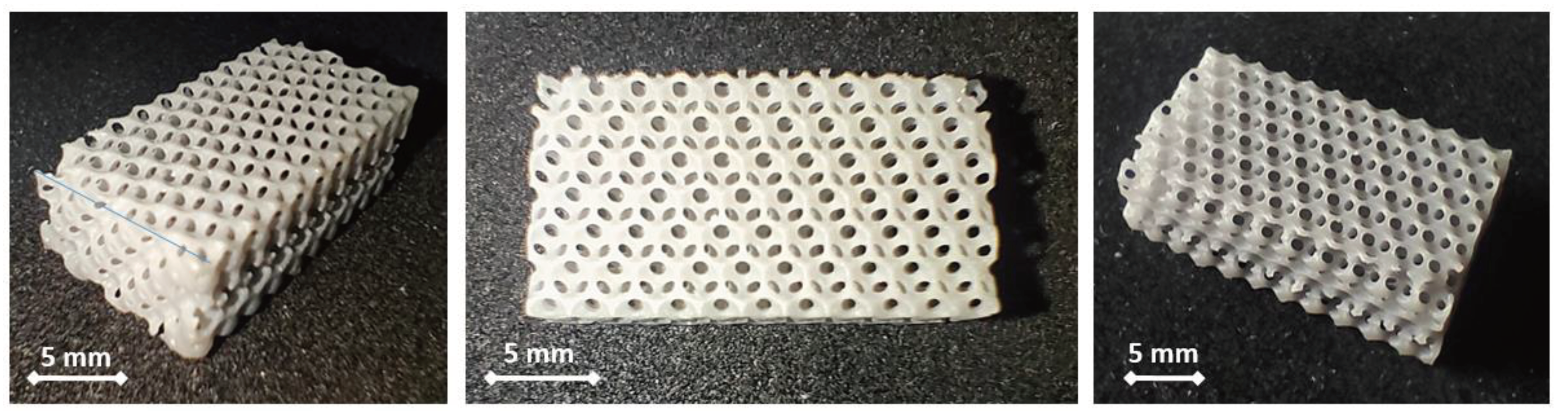
Figure 2.
Drawing of the micro-pores feature with variable diameter and SLA fabricated samples.
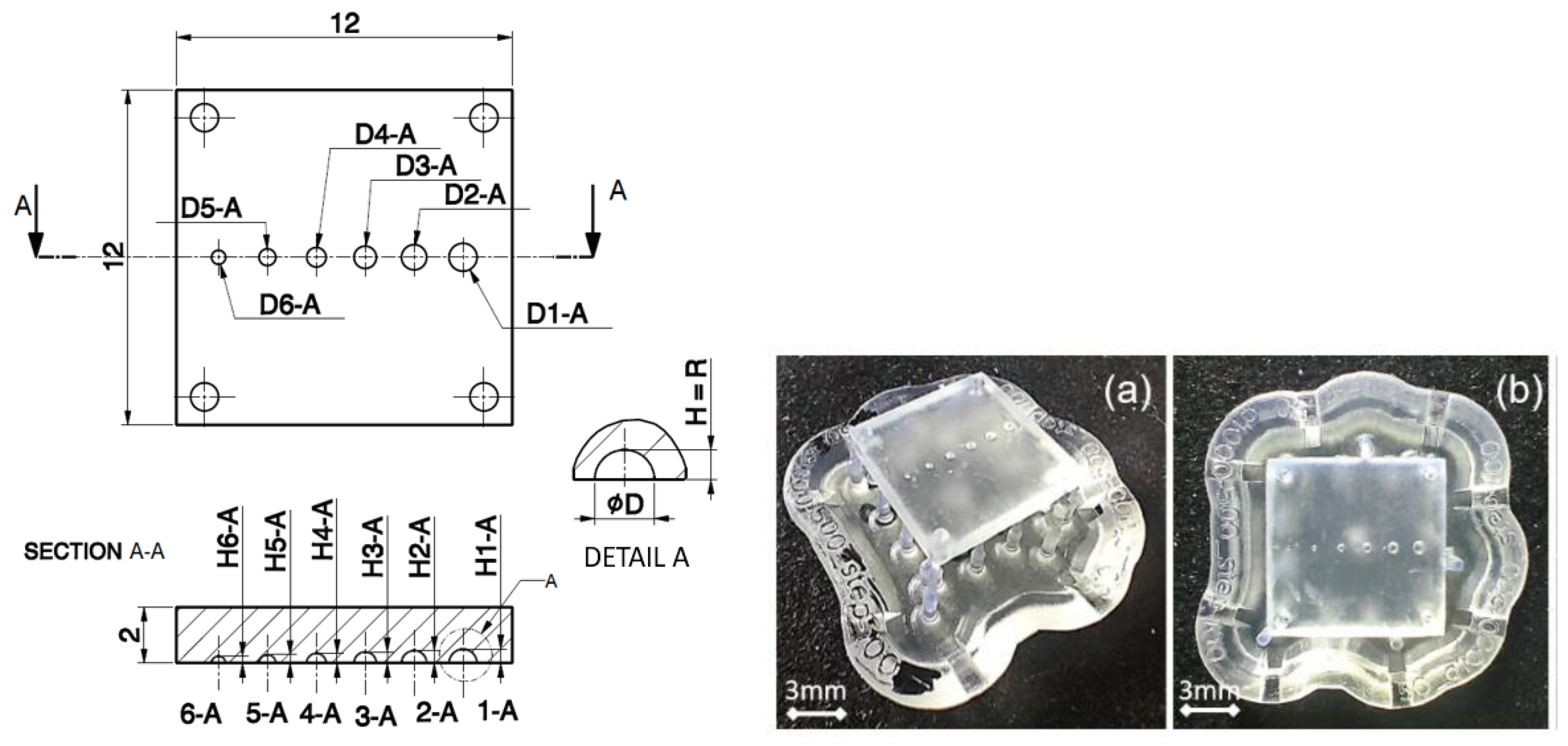
Figure 3.
Image processing of acquisition images. (a) Color threshold algorithm: parameters (top) and result (bottom); (b) Analyze particles algorithm: parameters (top) and result (bottom).
Figure 3.
Image processing of acquisition images. (a) Color threshold algorithm: parameters (top) and result (bottom); (b) Analyze particles algorithm: parameters (top) and result (bottom).
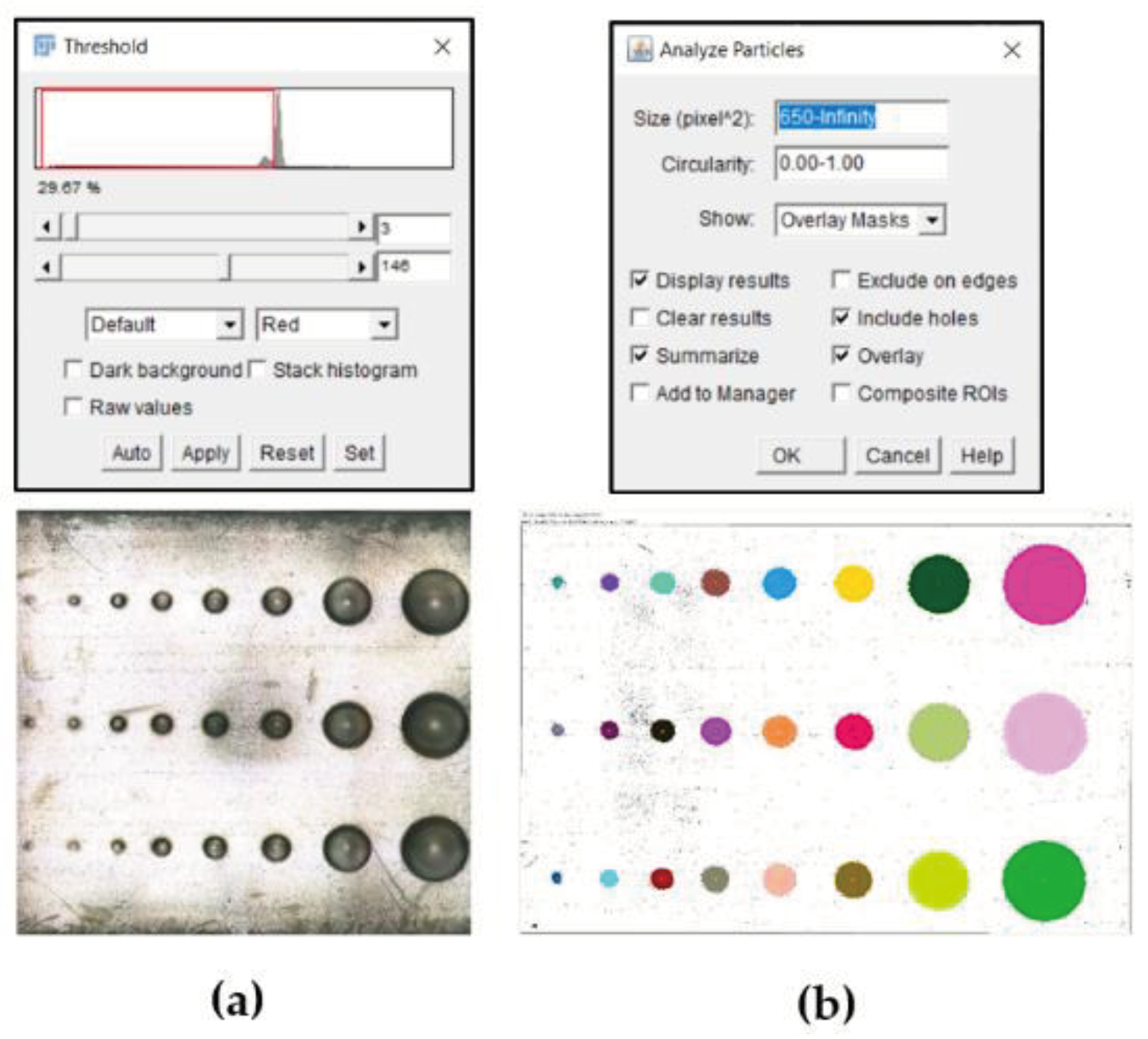
Figure 4.
Formlabs Preform slicing of the LPEP. (a) Part pre-processed into the virtual build volume: Images of a slice with holes (b–d) and protrusions (e,f). Hypothesis on layer UV-curing errors. Triangular hole (g) and protrusion (h). Nominal edges are depicted with a solid red line, also corresponding to the laser beam path; Actual UV-cured geometry (dashed black line); Bulk UV-cured region in blue color.
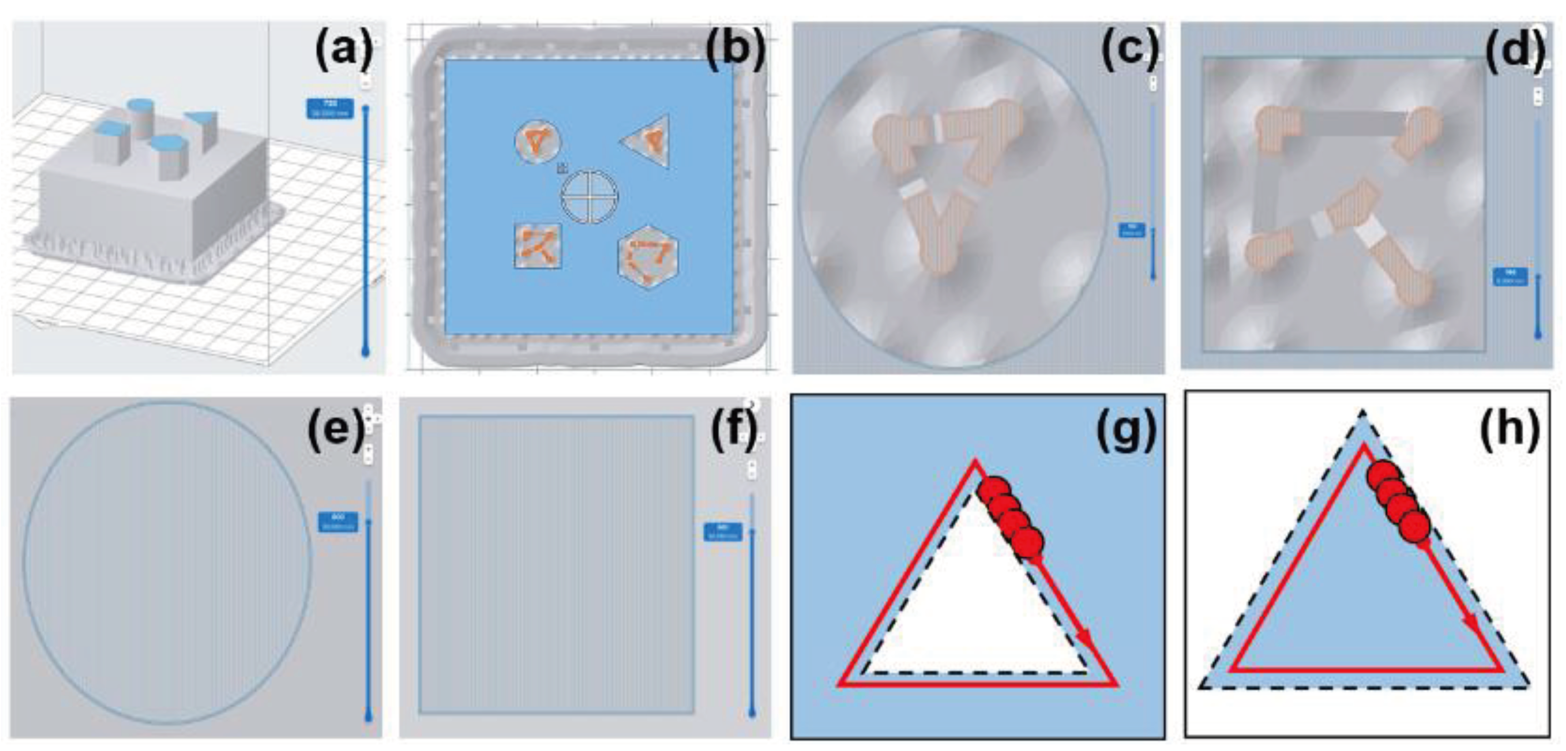
Figure 5.
Graphs of diameter (a) and depth (b) as a function of nominal values of the printed full-open micro-pores.
Figure 5.
Graphs of diameter (a) and depth (b) as a function of nominal values of the printed full-open micro-pores.
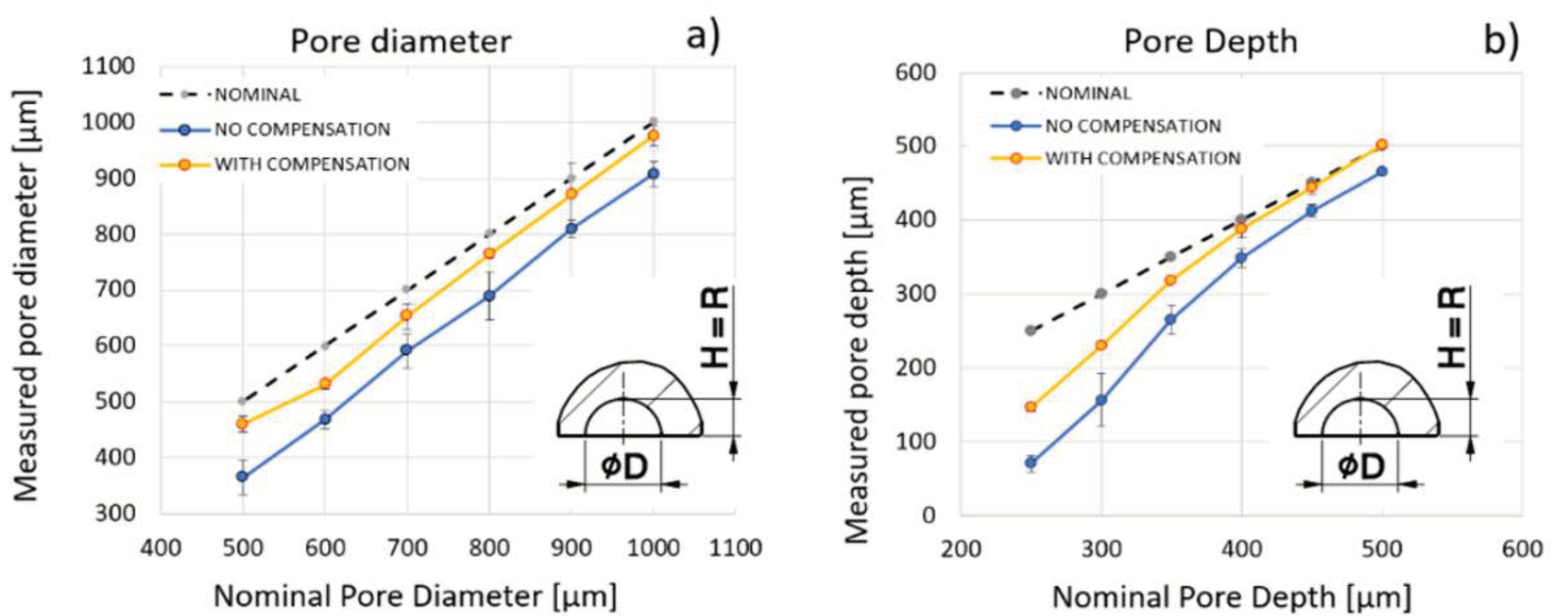
Figure 6.
Test part for the measurement of the correction parameter. (a) Drawing; (b) top view and (c) 3D view of the printed part samples.
Figure 6.
Test part for the measurement of the correction parameter. (a) Drawing; (b) top view and (c) 3D view of the printed part samples.
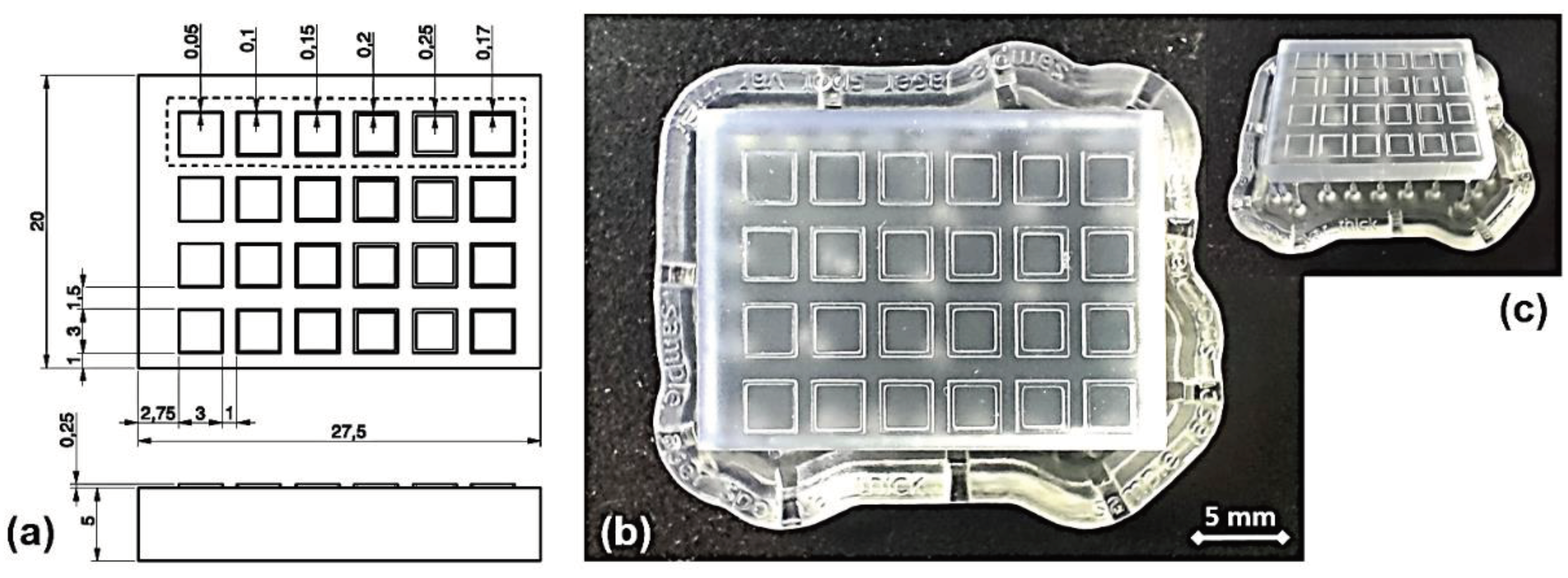
Figure 7.
Laser Spot Path for the wall infill: a) Wall Thickness of 150 µm; b) Wall Thickness of 200 µm.
Figure 7.
Laser Spot Path for the wall infill: a) Wall Thickness of 150 µm; b) Wall Thickness of 200 µm.
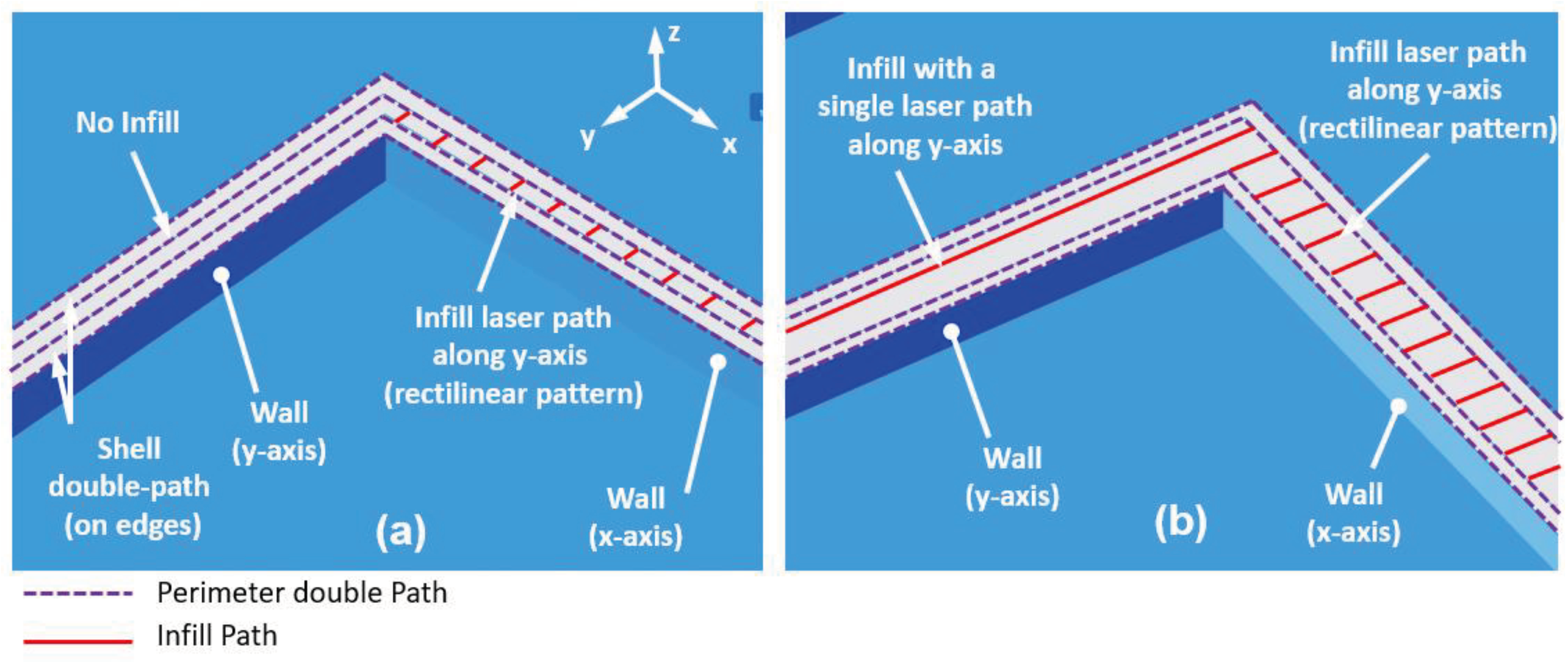
Figure 8.
Measures of thin wall thickness and laser beam spot diameter. (a) Graph of measurements; (b) Image of the profilometer acquisition.
Figure 8.
Measures of thin wall thickness and laser beam spot diameter. (a) Graph of measurements; (b) Image of the profilometer acquisition.
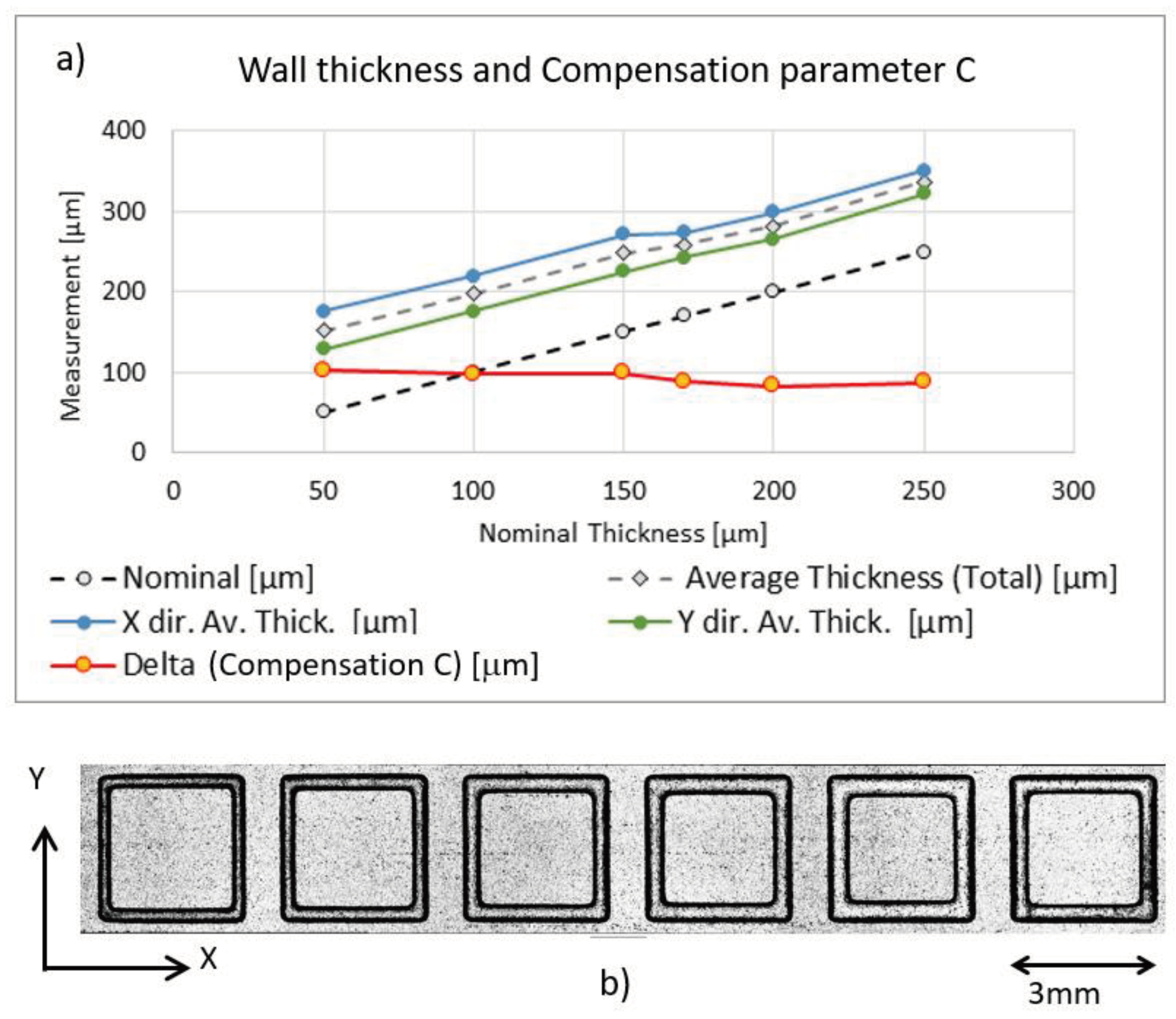
Figure 9.
Measures of thin wall thickness and C on a 45-degree 3D printing orientation. (a) Graph of measurements; (b) Part orientation in Preform environment; (c) detail of the laser infill paths; (d) Image of the Sensofar profilometer acquisition. Data and colors are the same of Figure 8.
Figure 9.
Measures of thin wall thickness and C on a 45-degree 3D printing orientation. (a) Graph of measurements; (b) Part orientation in Preform environment; (c) detail of the laser infill paths; (d) Image of the Sensofar profilometer acquisition. Data and colors are the same of Figure 8.
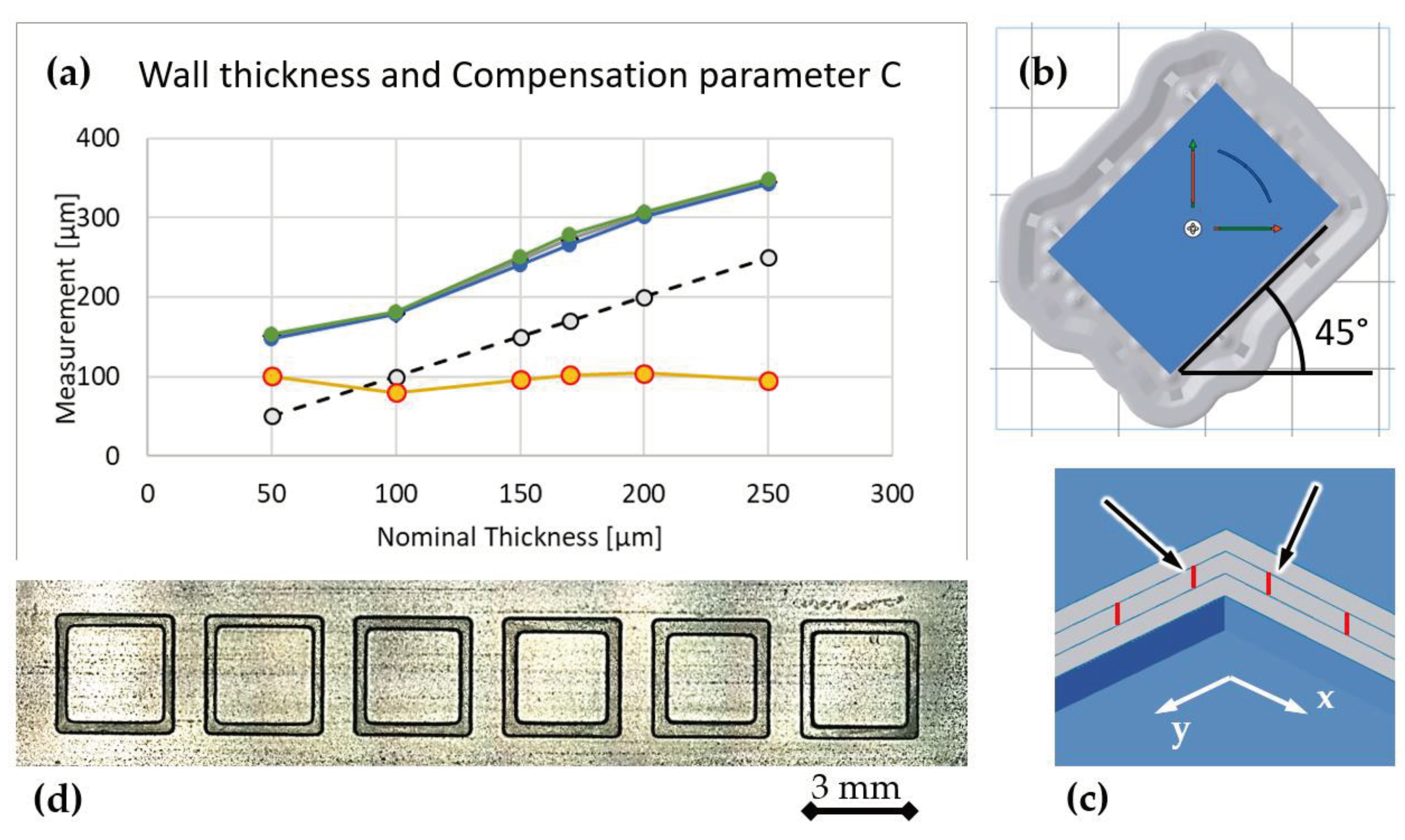
Figure 10.
Effects of the constant compensation strategy with different values of the compensation parameter: without compensation C=0 (blue line); with constant compensation C=85μm (orange line); C=96μm (purple line); C=120μm (yellow line).
Figure 10.
Effects of the constant compensation strategy with different values of the compensation parameter: without compensation C=0 (blue line); with constant compensation C=85μm (orange line); C=96μm (purple line); C=120μm (yellow line).
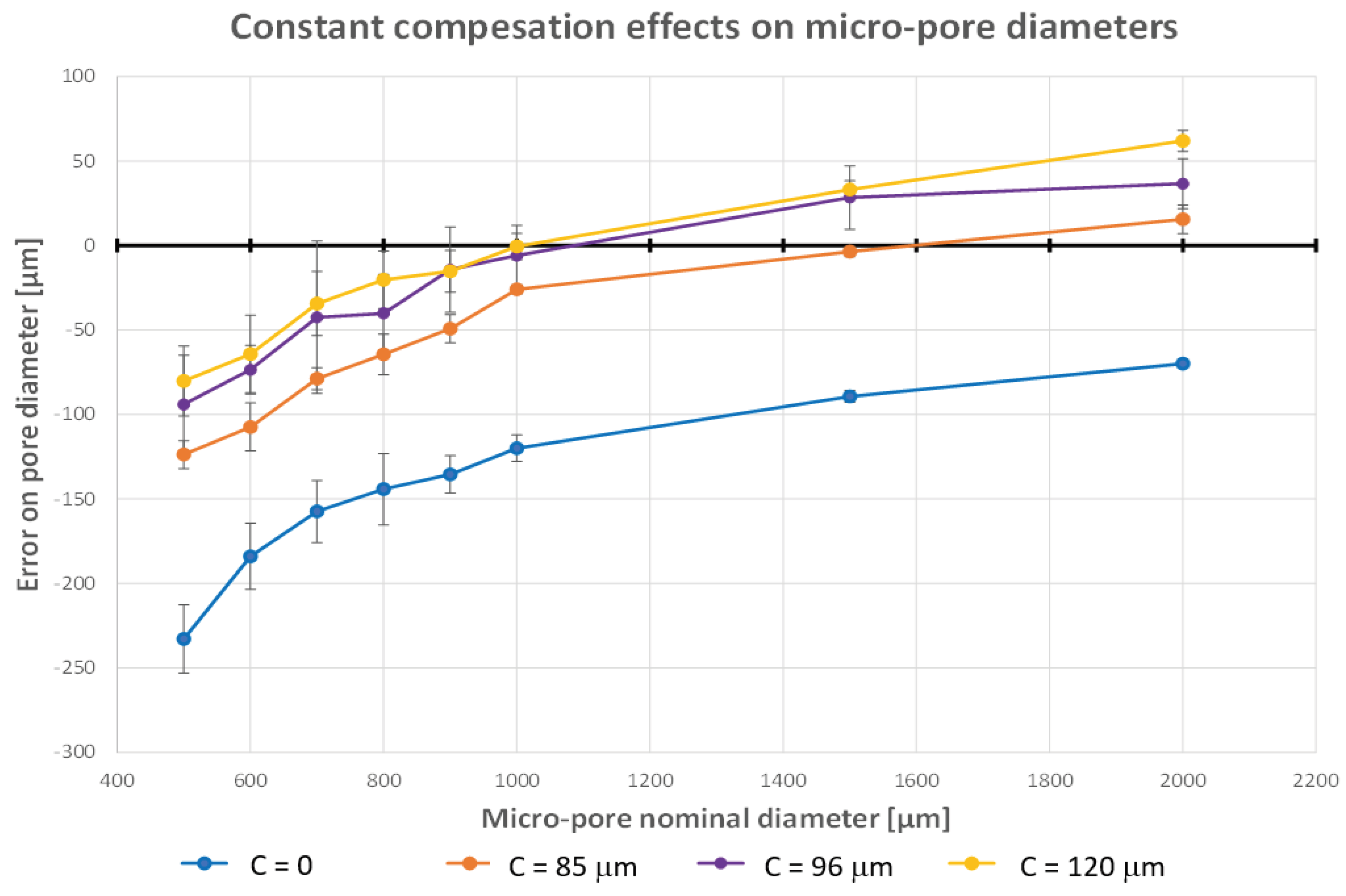
Figure 11.
Plot of all experimental data, identification of a second-order interpolation law and its solution. Nominal values of pore diameter (orange line); measured diameters (blue line) with data dispersion (standard deviation); Second-order polynomial interpolation (dashed blue line) and its equation y=f(x); Curve of compensation parameters (solid grey line).
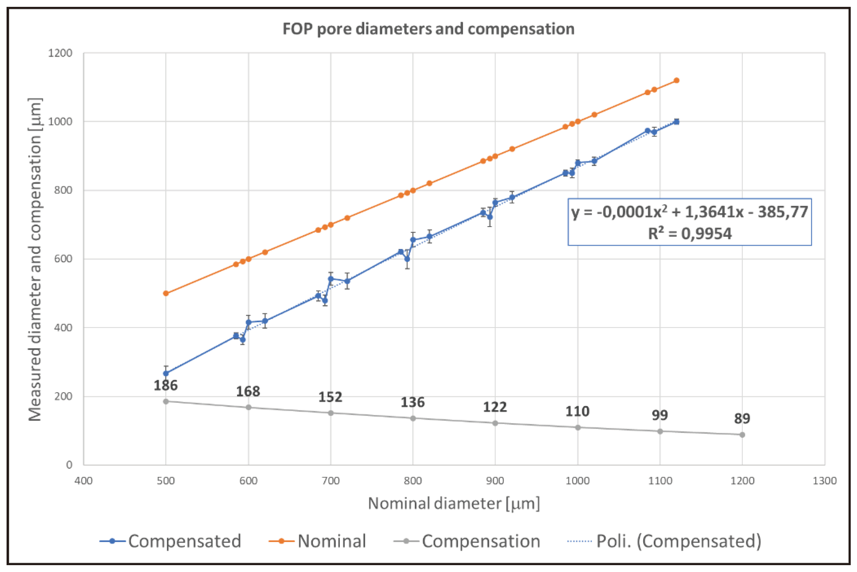
Figure 12.
Plots of model prediction, variable, and constant compensations. Model prediction (compensated values) of the diameters (blue line); model compensation (yellow solid line) and its 2nd-order interpolation (yellow dashed line) with its equation (inset); constant compensation equal to the nominal laser spot diameter (black dashed line).
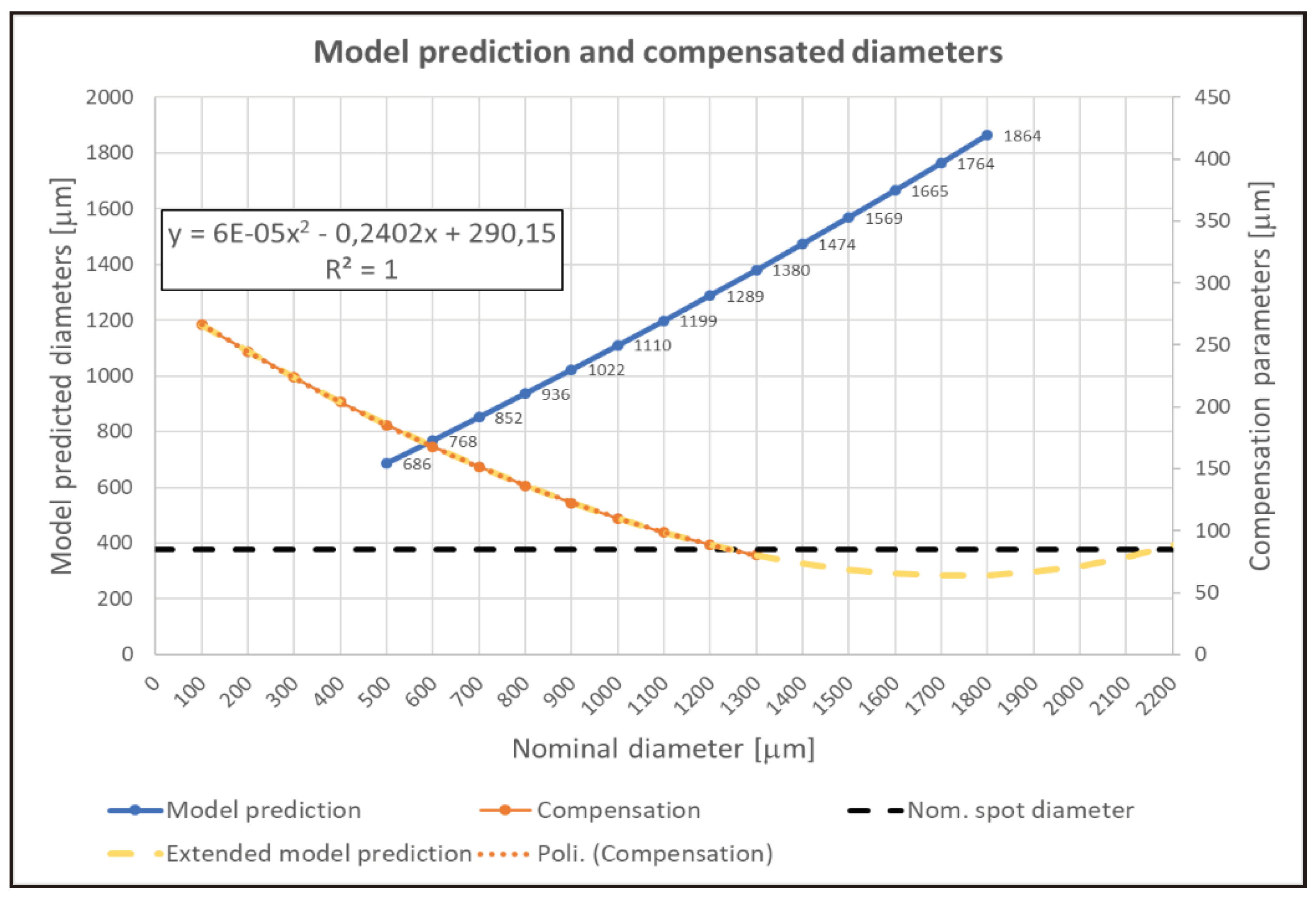
Figure 13.
Micro-pores sample drawings.
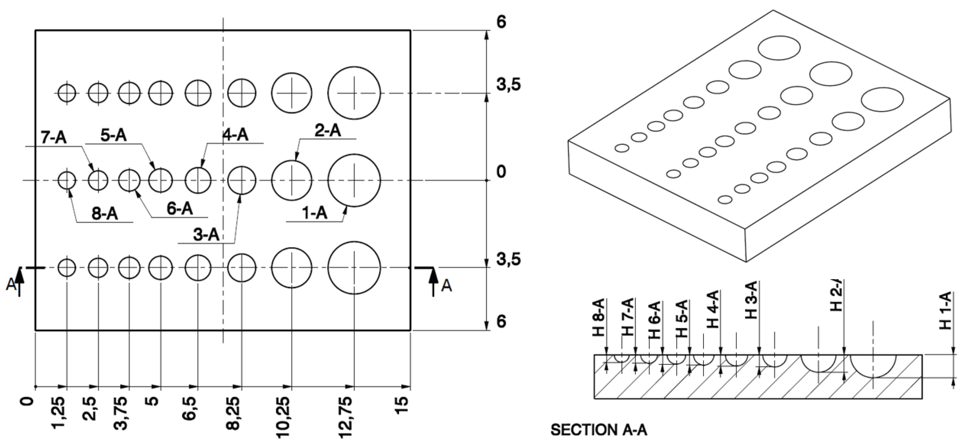
Figure 14.
Picture of the four samples with variable compensation. Each sample has three patterns of micro-pores with varying diameters, from 2mm down to 500μm.
Figure 14.
Picture of the four samples with variable compensation. Each sample has three patterns of micro-pores with varying diameters, from 2mm down to 500μm.
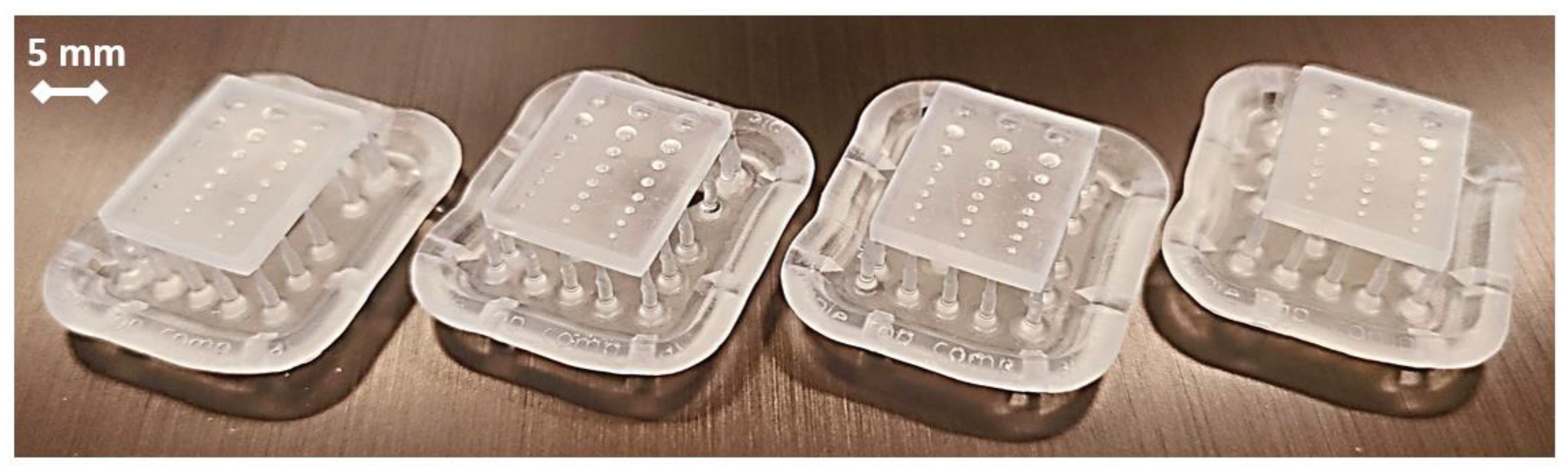
Figure 15.
Plots of the error percentage on pore diameters, without compensation (orange curve), with constant C=85μm (green curve) and variable compensations (blue and yellow curves).
Figure 15.
Plots of the error percentage on pore diameters, without compensation (orange curve), with constant C=85μm (green curve) and variable compensations (blue and yellow curves).
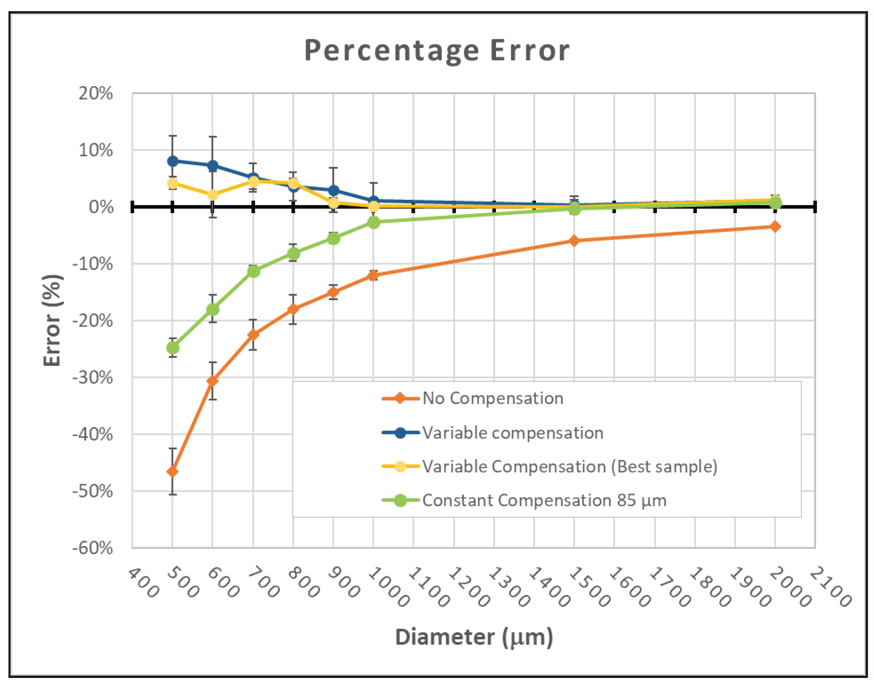

Table 1.
Nominal dimensions of FOP features (Figure 2).
Table 1.
Nominal dimensions of FOP features (Figure 2).
| Dimension | FOP Features | |||||
|---|---|---|---|---|---|---|
| (μm) | 1-A | 2-A | 3-A | 4-A | 5-A | 6-A |
| D | 1000 | 900 | 800 | 700 | 600 | 500 |
| H | 500 | 450 | 400 | 350 | 300 | 250 |
Table 2.
SLA process parameters.
| Parameter | Units | Values | Symbol |
|---|---|---|---|
| Layer Thickness | μm | 25 | LT |
| Support attachment point size | mm | 0.7 | SP |
| Support positions | - | Uniformly distributed | |
| Support points density. Index (0.5-1.5) | - | 1 (average 1.75 supports/10mm2) | SD |
| Base thickness | mm | 2 | BT |
| Min distance of the part from base | mm | 5 | |
| Part Orientations | - | horizontal & parallel to the build platform) |
Table 3.
Measurements of diameters and depths of the FOP.
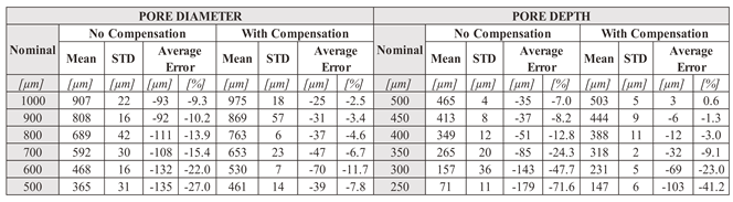 |
Table 4.
Wall thickness measurements and compensation parameter C estimation.
| Thin Wall | Nominal Thickness |
Thickness Along X-Axis |
Thickness Along Y-Axis |
Total Thickness | Compensation Parameter “C” | |||
|---|---|---|---|---|---|---|---|---|
| Mean | Error | Mean | Error | Mean | STD | |||
| # | [µm] | [µm] | [µm] | [µm] | [µm] | [µm] | [µm] | [µm] |
| 1 | 50 | 176 | 126 | 128 | 78 | 152 | 29 | 102 |
| 2 | 100 | 220 | 120 | 176 | 76 | 198 | 27 | 98 |
| 3 | 150 | 272 | 122 | 226 | 76 | 249 | 29 | 99 |
| 4 | 200 | 299 | 99 | 265 | 65 | 282 | 21 | 82 |
| 5 | 250 | 350 | 100 | 323 | 73 | 337 | 20 | 87 |
| 6 | 170 | 274 | 104 | 243 | 73 | 258 | 21 | 88 |
Table 5.
Thickness measurements of thin walls on a 45-degree orientation 3D-printed sample.
| Thin Wall | Nominal Thickness |
Thickness Along X-Axis |
Thickness Along Y-Axis |
Total Thickness | C = Actual DLS | |||
|---|---|---|---|---|---|---|---|---|
| Mean | Error | Mean | Error | Mean | STD | |||
| # | [µm] | [µm] | [µm] | [µm] | [µm] | [µm] | [µm] | [µm] |
| 1 | 50 | 147 | 97 | 154 | 104 | 150 | 8 | 100 |
| 2 | 100 | 178 | 78 | 181 | 81 | 180 | 6 | 80 |
| 3 | 150 | 241 | 91 | 252 | 102 | 246 | 15 | 96 |
| 4 | 170 | 266 | 96 | 279 | 109 | 272 | 9 | 102 |
| 5 | 200 | 302 | 102 | 307 | 107 | 304 | 13 | 104 |
| 6 | 250 | 343 | 93 | 348 | 98 | 345 | 9 | 95 |
According to these new experimental data and measurements, the actual value of C is estimated to be 96.2±8.6 μm.
Table 6.
Nominal and actual values of micro-pores dimensions and variable compensation factor.
| Dimension / Parameter | FOP Features | |||||||
|---|---|---|---|---|---|---|---|---|
| (μm) | 1-A | 2-A | 3-A | 4-A | 5-A | 6-A | 7-A | 8-A |
| Nominal Diameter DN | 2000 | 1500 | 1000 | 900 | 800 | 700 | 600 | 500 |
| Diameter compensation C | 96 | 96 | 110 | 122 | 136 | 152 | 168 | 186 |
| Compensated Diameter D=DN + C | 2096 | 1596 | 1110 | 1022 | 936 | 852 | 768 | 686 |
| Compensated Pore depth H = D/2 | 1048 | 798 | 555 | 511 | 468 | 426 | 384 | 343 |
Table 7.
Summary of results with constant and variable compensation strategy. Mean absolute and percentage errors.
Table 7.
Summary of results with constant and variable compensation strategy. Mean absolute and percentage errors.
| DN | No Compensation |
Constant Compensation | Variable Compensation | |||||||||
|---|---|---|---|---|---|---|---|---|---|---|---|---|
| C = 85 μm | C = 96 μm | C = 120 μm | All Samples | BEST Sample | ||||||||
| [μm] | [μm] | [%] | [μm] | [%] | [μm] | [%] | [μm] | [%] | [μm] | [%] | [μm] | [%] |
| 500 | -233 | -46.6 | -124 | -24.8 | -94 | -18.8 | -80 | -16.0 | 41 | 8.2 | 21 | 4.2 |
| 600 | -184 | -30.7 | -107 | -17.8 | -73 | -12.2 | -64 | -10.7 | 45 | 7.5 | 13 | 2.2 |
| 700 | -157 | -22.4 | -79 | -11.3 | -42 | -6.1 | -34 | -4.9 | 36 | 5.1 | 31 | 4.4 |
| 800 | -144 | -18.0 | -64 | -8.0 | -40 | -5.0 | -20 | -2.5 | 29 | 3.6 | 34 | 4.3 |
| 900 | -135 | -15.0 | -50 | -5.6 | -14 | -1.6 | -15 | -1.7 | 27 | 3.0 | 7 | 0.8 |
| 1000 | -120 | -12.0 | -26 | -2.6 | -6 | -0.6 | -1 | -0.1 | 12 | 1.2 | 2 | 0.2 |
| 1500 | -89 | -5.9 | -4 | -0.3 | 28 | 1.9 | 33 | 2.2 | 4 | 0.3 | 1 | 0.1 |
| 2000 | -70 | -3.5 | 15 | 0.8 | 37 | 1.8 | 62 | 3.1 | 22 | 1.1 | 36 | 1.8 |
Disclaimer/Publisher’s Note: The statements, opinions and data contained in all publications are solely those of the individual author(s) and contributor(s) and not of MDPI and/or the editor(s). MDPI and/or the editor(s) disclaim responsibility for any injury to people or property resulting from any ideas, methods, instructions or products referred to in the content. |
© 2024 by the authors. Licensee MDPI, Basel, Switzerland. This article is an open access article distributed under the terms and conditions of the Creative Commons Attribution (CC BY) license (http://creativecommons.org/licenses/by/4.0/).
Copyright: This open access article is published under a Creative Commons CC BY 4.0 license, which permit the free download, distribution, and reuse, provided that the author and preprint are cited in any reuse.
Submitted:
08 March 2024
Posted:
08 March 2024
You are already at the latest version
Alerts
A peer-reviewed article of this preprint also exists.
This version is not peer-reviewed
Submitted:
08 March 2024
Posted:
08 March 2024
You are already at the latest version
Alerts
Abstract
In this paper, we present an experimental procedure to enhance the dimensional accuracy of fabrication via Stereolithography (SLA) of features at the micro-scale. Using a custom benchmark part, deviations in feature dimensions (micro-pores diameters and depths) were detected and measured by confocal microscopy. Samples characterization and experimental observations allowed the identification of inaccuracy sources, mainly due to the laser beam scanning strategy and to the incomplete removal of uncured liquid resin in post-processing (i.e., IPA washing). As a technology baseline, the measured dimensional errors on pores diameters were up to -46%. A compensation method of the nominal laser spot diameter (85m) was defined and implemented resulting in relevant improvements in dimensional accuracy of 9.8% and 11.3% on full-open pores diameter and depth, respectively. Further investigation was performed on a customized test part to adjust the calibration procedure. The measurements revealed that the estimate of the laser beam spot size is 968m. Measurements on micro-pores having different sizes revealed that a constant compensation parameter (i.e., C=85, 96, 120m) is not fully effective at the micro-scale, where average errors still remain at -24%, -18.8%, and -16% for compensations equals to 85, 96 and 120m, respectively. A further experimental campaign allowed the identification of an effective nonlinear compensation law where the compensation parameter depends on the micro-feature size C= f (D). Results show a sharp improvement in dimensional accuracy on micro-pore fabrication, with errors consistently below +8.2%. The proposed compensation method can be extended for the fabrication of any micro-features without restrictions on the specific technology implementation. Concerning the inaccuracy introduced by the laser path, experimentation with a customized part allowed the optimization of the part orientation to reduce the errors and their differences along the X and Y machine axes.
Keywords:
Subject: Engineering - Industrial and Manufacturing Engineering
1. Introduction
Among Additive Manufacturing (AM) technologies, Stereolithography (SLA) is largely used to fabricate parts with intricate 3D geometry, and very accurate features, due to its performance, high speed, resolution, high precision, smooth finishing, low waste, and affordability of polymers, composites and ceramics materials, with a fully-digitalized process [1]. SLA belongs to the family of VAT Photo Polymerization (VPP) technologies, and it exploits liquid photopolymers, which are polymerized by a laser beam spot (LBS) that scans and UV-cures the material, layer by layer.
The SLA process with its variants (top-down and bottom-up exposure) is, among other applications, successfully used to fabricate regular/high-ordered porous 3D microstructures [2,3]. Figure 1 shows an inverse opal, a face-centered cubic structure (FCC), fabricated via bottom-up SLA.
Several studies were conducted with different objectives: development of advanced applications, process parameters optimization, investigation of new materials performance and processability, addressing technology issues and process sustainability, conceiving innovative process chains, etc. [4,5,6,7,8]. Remarkable achievements were obtained by investigating SLA process parameters aiming at identifying their effects on the 3D-printed part quality: dimensional accuracy, surface finishing, mechanical properties, defects occurrence, etc. Sabbah A. et al. [9] found a negligible impact of the layer thickness (LT) on surface finishing, while it strongly affects the dimensional accuracy of 3D-printed parts. The minimum layer thickness of 25μm resulted in higher precision. Cotabarren, I. et al., confirmed that layer thickness is a critical parameter for part accuracy; measurement deviation was reduced by about 90% when this parameter was reduced from 100 to 25μm [10].
Arnold C. et al. [11] concluded that the surface roughness of 3D-printed parts is firmly dependent on the model orientation in the build volume. The best results were obtained with a 0-degree part orientation (surface lies horizontally on the build platform) with measured values of Ra=1.15±0.47 μm along the X-axis and Ra=0.90±0.33 μm along the Y-axis. Other similar studies confirmed these results [12]. Shanmugasundaram S. et al. investigated the effects of printing orientation on the part’s mechanical properties, and no significant anisotropy was detected thanks to UV-curing post-processing [13]. Hada, T. et al. found that the highest dimensional accuracy is achieved by orienting the part with a 45-degree angle on the build platform, followed by a 90-degree orientation. The worst orientation is the 0-degree with the part parallel to the build platform [14]. These results were also confirmed by other studies [15,16].
As it can be noticed, several works focused on the influence of process parameters on the quality of 3D-printed parts, but there is a lack of research studies on the effects of the laser-scanning path and post-processing operations on the feature accuracy, especially at the micro-scale.
An original approach was implemented by Wen C. et al. [17], who investigated the geometric accuracy of microstructures of a Projected SLA, also known as Digital Light Processing (DLP) technology. They identified a compensation method of inaccuracy introduced by the light power intensity distribution. The proposed solution is based on structure optimization using a compensation parameter derived by the simulation results. The micro-features design (circles, squares, and triangles) is modified in dimension and shape to increase the dimensional accuracy. This compensation strategy allows the achievement of a mean error reduction from 21-23% down to 1.6-4.8%.
In the present study, the dimensional accuracy of the manufacturing of micro- features and structures via SLA technology was investigated and an approach for inaccuracy compensation has been conceived and tested. It is an extension of a previous preliminary study [18]. The laser beam spot and laser path were experimentally analyzed and inaccuracy sources were identified and addressed. The investigation revealed that a considerable part of the geometrical error was related to the laser path. However, by decreasing the feature’s size other phenomena become more important. Therefore, the study focused on two main aspects: i) laser path improvement; ii) identification of a compensation factor that considers both an estimation of laser beam spot diameter and other phenomena that affect the geometrical accuracy. The technology limitation was evaluated, and effective solutions were proposed, thus increasing the SLA capability and accuracy of the fabrication of micro-features at the micro-scale.
2. Materials and Methods
Micro-pore features are the fundamental component of all porous materials, as a single feature (1D), or replicated in a surface texturing (2D planar or freeform patterns) or in a volume (3D). In the latter case, if the pores are regularly distributed along the three directions in a pattern, the resulting structures are lattices. All these cases are characterized by a single pore or a single cell, including pores and fractions of pores. For this reason, the proposed approach investigates the fabrication of a single pore and its accuracy. The investigation on the fabrication by SLA of porous micro-features was performed by designing a sample with Full-open pores (FOP), thus hemispherical cavities, with variable diameters from 1 mm (1-A) down to 0.5 mm (6-A) with a step of 100 μm (Figure 2) and reported in Table 1. Figure 2 also shows the SLA fabricated samples before the detachment from the base and supports.
Each geometry was realized in three samples with the parameters reported in Table 2. The equipment adopted for fabricating the samples is a Formlabs Form 3 (Formlabs Inc., USA), having a build volume of 145×145×185 mm3, equipped with a class 1 violet laser emitting at a wavelength of 405nm with a nominal laser beam spot diameter DLS of 85 μm and a power of 250 mW. The positioning resolution on the x-y plane is 25 μm, while the z-axis resolution can be set from 200 to 25 μm (layer thickness). Samples were designed with the 3D CAD Solidworks 2017 (Solidworks Corp., Dassault Systèmes, USA), exported to Stereo Lithography interface (STL) format, and then imported into the Formlabs slicing software Preform v.3.32.0. In this software environment, parts were oriented, and all the process parameters were chosen according to the database supplied by the machine manufacturer and to previous studies [6,12,19]. The surface with micro-pore features was oriented horizontally, thus parallel to the build platform, which guarantees a higher surface finishing [12,19]. The process parameters are reported in Table 2.s
Samples were fabricated in Formlabs Clear V04 photopolymer resin, identified by the manufacturer’s code RS-F2-GPCL-04 [20]. After the SLA processing, parts were removed from the build platform and washed for 20 minutes into high-purity 99% isopropyl alcohol (IPA) and 5 minutes with ultrasound washing. Samples were acquired with an optical profilometer Sensofar S-Neox (Sensofar group, Barcellona, Spain), set with a Focus Variation acquisition method, using an objective EPI 10X with numerical aperture NA of 0.30 and a pixel resolution of 1.29 µm. Acquired images were processed by means of algorithms of the ImageJ software (National Institutes of Health NIH, USA) version 1.54g. The images were processed using a “threshold” (Figure 3a) and a “analyze particles” (Figure 3b) algorithms. This image processing procedure automatically gives several parameters regarding the shape (such as roundness, circularity, and solidity indexes) and size (such as area, perimeter, width, and height) of the region of interest (i.e., cavity or particle). The average diameter of each pore is calculated by the measured area using the formula: Diameter = .
2.1. Effect of the Laser Scanning Path
In order to investigate the effects of the laser beam path generation on the final part accuracy, a specific component, referred to as Laser Path Evaluation Part (LPEP), was designed with both simple holes and protrusions. The CAD model was then imported into the Formlabs Preform slicing software and the laser path was generated. The LPEP was oriented flat on the build platform (horizontal, Figure 4a) and preprocessed with the Preform algorithms to generate base, supports, slicing, and laser beam paths (Figure 4b). Figure 4 reports the slicing and laser beam paths of circular and squared holes (Figure 4c,d) and protrusions (Figure 4e,f). Looking at the generic slice of the region with holes, it can be easily recognized that the laser beam path starts exactly on the hole edge, and it proceeds with a double-contour path of the 2D-slice geometry. This step of the layer curing strategy is also referred as the “perimeter” step. The bulk material, which is the external region of the hole, is then UV-cured by a rectilinear infill with linear parallel laser beam paths and a distance between them likely equal (or slightly smaller) to the nominal laser spot diameter. The same observations can be done looking at the protrusion features. The laser beam path contours the protrusion edges towards the material side with two contours or perimeters, the first on the protrusion edge and the second with an offset from the first. The internal region of the protrusion is filled with a rectilinear path oriented according to the part orientation (see Figure 4).
The hypothesis is the following. If the circular laser spot, having a diameter of DLS, is centered on the line path, then all the edges of the slices, no matter if hollowed or protrusions, will be affected by an over-polymerization equal to the laser spot radius on each side or edge. This will result in smaller holes and larger protrusions than nominal ones. Each laser spot polymerization of the current layer has a volume that can be approximated to VLS=DLS*LT, and the over-polymerized volume equal to DLS*LT/2 will occur along the edges. Of course, at the meso and macro-scale, this inaccuracy is not relevant since it is a small percentage of the nominal dimensions, but it is very important at the micro-scale, where nominal dimensions are of the same order as the laser beam spot diameter. The hypothesis is schematized in Figure 4g,h).
If this hypothesis is confirmed, then inaccuracy occurs due to the missing compensation of the laser spot radius in the laser path generation algorithm, and a compensation method can be developed and applied. Since it is not possible to modify the laser path in the Preform slicing software, an effective strategy consists in applying an offset volume to the 3D models, i.e., as a general rule, by increasing the cavities and by reducing protrusions. The offset value should be carefully identified. In the simple case of hemispherical pore micro-features, the compensation to the model pore diameter is DP =DNP+C, where DNP is the nominal pore diameter, and C is the compensation parameter.
In order to investigate other sources of inaccuracy, Section 3.1 presents a preliminary test considering the designed FOP pore micro-features without and with compensation. Further investigations were executed to achieve an empirical esteem of the parameter C. Results are presented in Section 3.2. The effects of the constant compensation strategy with different values of the compensation parameter are discussed in Section 3.3. Finally, a deep analysis of the experimental data suggested a calibration procedure based on a variable compensation parameter taking into account the dependency of C from the feature size (i.e., micro-pore diameter). The procedure and results are presented in Section 3.4.
3. Results and Discussion
3.1. Preliminary Test: Measurements of Full-Open Micro-Pores (FOP)
Preliminary tests are performed by 3D printing the designed FOP micro-features without and with the compensation C, defined as equal to the nominal laser beam spot diameter DLS=85μm. The diameters and depths measurements of micro-pores are reported in Table 3 with their mean values and standard deviations; the same data are shown in Figure 5.
The average error on pore diameters spans between -92 and -135 µm, and it is consistent (in value and sign) with the hypothesis of missing compensation of the laser beam spot radius on contours. Further confirmation arises from the measured diameter considering a compensation C= 85µm, increasing the pore dimension accordingly. In this latter case, the reduced error spans between -25 and -75 µm. It is also possible to observe that the error increases when the pore diameter decreases. This behavior can be attributed to the adhesion of the uncured liquid resin on the solid surface due to surface tension, whose effect increases as dimensions decrease and becomes evident for cavities with sub-millimetric diameters. Thus, the IPA washing aimed at removing uncured resin residuals is less effective on pores at the micro-scale, preventing the fabrication of micro-cavities below a threshold size.
The depth of the pores is affected by an average error that spans between -35 and -179µm, which is reduced when the compensation is adopted, varying between 3 and -103µm. The compensation has a beneficial influence on the depth error because it enlarges the cavity, producing two effects: it dampens the cutoff of the geometry slicing and reduces the resin adhesion effect.
3.2. Esteeme of the Compensation Parameter
The preliminary test reveals that the error in diameter is not fully compensated by adopting C equal to the nominal laser spot diameter, also at a millimetric scale.
An assessment of C has been attempted by printing and measuring the part shown in Figure 6, which presents four repetitions of six squared thin wall features. The wall thicknesses vary in the following sequence: 0.05, 0.1, 0.15, 0.2, 0.25, and 0.17 mm.
Since slicing always has two paths on the edges of each thin wall, a feature with a wall thickness equal to two times the laser beam spot nominal diameter (170μm) was added at the end of the pattern. Figure 6a shows the drawing of the proposed part for the correction factor estimation. Samples were fabricated according to the described conditions (Section 2) and parameters (Table 1). A sample of the part is shown in Figure 6b,c.
The difference between the nominal and the measured wall thickness returns an estimate of how much the geometrical edge must be moved (offset) to achieve the complete compensation. The measurements are reported in Table 4 with the estimated value of C.
The C value ranges between 88 and 102 µm, with an average value of 93 µm and a standard deviation of 8 µm. It must be observed that the average value tends to be greater than the nominal diameter of the laser spot (85 µm), with a growing trend when the wall thickness is thinner. This latter effect seems to be related to the step-over of the two on-edge laser paths (squares from 1 to 3), which increases when the wall thickness decreases. The high values of standard deviations are attributed to the different infill of the wall when the thickness increases at higher values (squared walls 4, 5, and 6). In fact, in these cases, when the wall thickness is higher than the laser beam spot diameter, the infill strategy is a rectilinear scan oriented along the machine y-axis. With this evidence (Figure 7), all walls oriented along the x-axis are filled with a pattern of parallel lines orthogonal to the wall edge. In contrast, all walls oriented along the y-axis are filled with additional lines along the wall edge.
Therefore, this different infill strategy determines different UV-curing for the same walls with related variable thickness, thus higher values of standard deviations in measurements. Figure 8 reports the graph of measurement of thin wall thicknesses and the estimated compensation parameter C. Nominal values of thin walls are represented by the slanted black dashed line. All deviations from this line are fabrication errors to be quantified. The values of the actual thin wall thicknesses along x- and y-axis are depicted with blue and green solid lines, respectively.
All measured thicknesses are higher than the nominal ones. The average wall thicknesses are depicted with a gray dashed line. As can be seen in the figure, wall thicknesses along the x-direction (blue line) are greater than those along the y-axis (green line), but the difference between them decreases beyond the threshold value of t*=150 μm. The differences between measured and nominal values are reported with an orange line.
As observed before, the estimated C is almost stable to about 100 μm up to the t*, and it decreases to 82-88 μm with thicknesses higher than t*. Indeed, up to t*, the infill is missing along the y-direction, while it is always present along the x-direction. The infill strategy significantly affects wall thickness accuracy, producing a different wall thickness depending on the wall orientation and nominal thickness, as shown in Figure 8.
The error on the thin wall thickness is 74±4.5 µm and 112±11.9 µm along the y- and x-axis, respectively. The graph in Figure 8 shows that the error on the wall thickness along the x-axis (blue line) is slightly reduced when its value is greater than 170μm, two times the nominal laser spot diameter. These data suggest that the current infill strategy produces geometrical anisotropy on features. Therefore, the part orientation on the XY plane affects the geometrical accuracy at the micro-scale. A different infill strategy (i.e., offset of the external perimeter) can improve the geometrical accuracy and reduce the anisotropy. More easily, an effective strategy to compensate for this anisotropy is an optimized orientation of the part on the build platform. Since the on-use machine allows only y-axis linear infill, an effective solution is a 45-degree orientation of the part on the XY plane (build platform).
Figure 9 shows the results obtained with the 45-degree orientation. The plot of the thin-wall measurements is depicted in Figure 9a, while a picture of the confocal acquisition is reported in Figure 9d. This part orientation (Figure 9b), generates linear infill patterns (red lines in Figure 9c) inside the wall thickness, which results in a sharply reduced anisotropy: same thickness (and error) along both the x- and y-axis. In fact, as it can be seen in Figure 9a, the graph lines (green and blue) of measurements along the two axes are almost superimposed but still exhibit an error due to the missing compensation. Four samples were 3D-printed at different positions on the build platform. The measurements and statistical values are reported in Table 5.
3.3. Constant Compensation Strategy
Since variability in the esteem of C has been found, the constant model compensations strategy was applied to the micro-pore diameters considering three levels of compensation:
- C=+85 μm, is equal to the nominal laser spot diameter;
- C=+96 μm, is the value obtained with the calibration tests;
- C=+120 μm, value identified as the average error on diameter obtained in the preliminary tests when the compensation of +85μm was applied.
Figure 10 shows the effects of the constant compensation strategy compared with the curve obtained without compensation.
As can be seen from the figure, the constant compensations – the same value of the parameter C for all pores – are not fully effective, especially at the small scale (diameters below 1,2 mm), where the error dramatically increases. The smaller the micro-pore, the higher compensation is required. Furthermore, the value of C=120μm produces an overcompensation (positive errors) for feature diameters higher than 1.0 mm, and similar results are obtained with C=85μm for feature diameters higher than 1.6 mm.
From these results, it can be concluded that inaccuracy related to the laser spot diameter is the most important and can be effectively compensated for pore dimensions down to about 1.2 mm. When the pore diameter gets smaller and smaller, other phenomena become more dominant, and the constant compensation is no longer effective. However, a strategy of variable compensation based on the feature size and the error trend can be investigated in order to empirically compensate all the sources of inaccuracy.
3.4. Variable Compensation Strategy
The results presented in the previous section clearly suggest that a nonlinear compensation law could be more effective than a constant or a linear compensation strategy as the pore dimension decreases to take into account phenomena typically arising at the microscale, such as adhesion and surface tension.
The nonlinear compensation law can be derived by processing the experimental data set. Its identification was performed by following three steps:
- Plot of all measurements of features on samples (i.e., FOP pore diameters), with and without compensations;
- Identification by polynomial regression of a mathematical relationship between actual and nominal values of the meso- and micro-feature size;
- Solving the equation obtained in the previous step, thus the value of the compensation parameter can be derived as a function of the feature size C = f(D) (i.e., pore diameter).
According to this procedure, data of nominal and actual diameters were plotted and analyzed. The polynomial model order for data identification was chosen as a trade-off between the mathematical complexity and the statistical confidence (coefficient of determination R2) in the model’s data prediction. A second-order polynomial interpolation model (three parameters) was identified by the Microsoft Excel regression algorithm, resulting in a value of R2=0.9954, which was considered satisfactory for the objective of the work. The model equations (explicit and implicit forms) are given by:
where y is the actual (measured) diameter, x is the related nominal diameter, and (a, b, c) are the parameters of the 2nd-order polynomial regression model. The values of the model parameters are: a = -0.0001; b = 1.3641; c = -385.77. The equation (1) was solved to obtain the nominal (compensated) values (x) of diameters that give the desired (y) values. Finally, the values of the required compensation parameter C are calculated as the difference between the measured and the compensated values of the pore diameters:
The model prediction of diameters and the related compensations were plotted on an extended and denser range of the nominal diameters (Figure 12). The curve of the variable compensation parameter (yellow line) reveals that for bigger features (diameters bigger than 1.2 mm), the compensation has values close to the constant nominal compensation and does not vary significantly. For this reason, at the meso scale, a variable compensation is not required, and a constant compensation strategy can be adopted. Therefore, it can be concluded that a discontinuity occurs in the compensation law: variable compensation at the micro-scale, down to D’=1200μm and a constant compensation law beyond this threshold.
Four samples were 3D-printed at different positions on the build platform in order to explore the possible effects of this parameter on data dispersion and part accuracy (Figure 14). Each sample reports a pattern of three sequences of full-open pores with eight target diameters in the range 500-2000μm. The compensation parameter for diameters higher than 1200μm was set to 96μm, thus the estimated value of the laser spot diameter obtained in Section 3.3. The drawing of the samples is depicted in Figure 13, and the nominal value of diameters and compensation parameters are reported in Table 6.
The error percentages calculated on sample measurements with their dispersions are reported in Figure 15. The curve of variable compensation (blue line) reveals a sharp improvement in accuracy with errors below 8.2%. The best sample error (yellow curve) is always below 4.4%. A slight overcompensation occurs at the micro-scale (below 900μm). Furthermore, a constant compensation strategy beyond D=1200μm is confirmed to be the best choice.
Table 7 reports mean errors and standard deviations without compensation and with constant and variable compensation.
As can be noticed, the absolute and percentage errors progressively decreased from no compensation to variable compensation. Also data dispersion has been improved. These results demonstrate that a compensation strategy increases the accuracy of technology, especially at the micro level. Furthermore, a variable compensation method based on the feature dimension is successful since it allows further improvement compared to the constant compensation strategy.
4. Conclusions
In this study, an SLA process was analyzed in terms of dimensional accuracy addressing micro-feature fabrication by investigating the effects of inaccuracy due to scanning paths, laser spot compensation, and post-processing operations. This analysis brought up that the accuracy of the fabrication can be improved introducing a compensation factor for the laser spot diameter and for the laser scanning path generation. The first attempt promoted in this work was a constant compensation applied to the part 3D model based on the nominal laser beam diameter, which is 85μm for the used equipment. This method increased the accuracy up to 20% and 30% on micro-pore diameters and depths, respectively. A benchmark test part was then conceived and used to estimate the actual compensation parameter, estimated as 96±8 μm, with a deviation of +12.9% from the nominal value.
The constant compensation strategy succeeds at the meso scale (i.e., D>1200μm), but fails at the micro-scale (i.e., D=500÷1200μm), where the dimensional accuracy remains low: error percentage up to 24.8%. This not negligible error is attributed to uncured resin, which remains trapped in the micro-pores where the removal by IPA washing is less effective. The analysis of the experimental data revealed that a variable (nonlinear) compensation method with the compensation parameter as a function of the micro-feature size (i.e., micropore diameter) is more suitable and effective. The variable compensation law for micro-pores was derived by the analysis of the experimental data obtained in the previous steps. A second-order polynomial regression law was used to obtain the nonlinear compensation with confidence of R2=0.9954. According to this new strategy, a final experimental campaign was performed. Measurements of samples showed a relevant increase in accuracy on micro-pore diameter, with an error percentage below 8.2%.
Regarding the technology, this study suggests improvements of the path generation strategy by compensating the actual laser spot diameter and optimizing the infill strategy.
This study focused on simple spherical micro-porous, and it did not consider complex geometries, which can require a challenging assessment to identify the correct compensation laws along the three axes. Other aspects to be investigated are the role and effectiveness of the IPA-washing post-processing, surface tension, and photopolymer viscosity in eliminating the trapped liquid resin into micro-pores and porous structures.
Author Contributions
Authors F.M. and V.B. contributed equally. Conceptualization, methodology, software, validation, writing—original draft preparation, F.M. and V.B.; writing—review and editing, V.B., F.M. and I.F.; supervision, I.F.. All authors have read and agreed to the published version of the manuscript.
Funding
This work was partially supported by the European Union under the Italian National Recovery and Resilience Plan (NRRP) of NextGenerationEU, a partnership on “Telecommunications of the Future” (PE00000001 - RESTART) and on “Made in Italy Circular and Sustainable” (PE00000004-MICS). This manuscript reflects only the authors’ views and opinions, neither the European Union nor the European Commission can be considered responsible for them.
Conflicts of Interest
The authors declare no conflict of interest.
References
- Kafle, Abishek, et al. “3D/4D Printing of polymers: Fused deposition modelling (FDM), selective laser sintering (SLS), and stereolithography (SLA).” Polymers 13.18 (2021): 3101.
- Bártolo, P. J., ed. Stereolithography: materials, processes and applications. Springer Science & Business Media, 2011.
- Zhang, F., et al. “The recent development of vat photopolymerization: A review.” Additive Manufacturing 48 (2021): 102423.
- Maines, Erin M., et al. “Sustainable advances in SLA/DLP 3D printing materials and processes.” Green Chemistry 23.18 (2021): 6863-6897.
- Muldoon K.et al.”High Precision 3D Printing for Micro to Nano Scale Biomedical and Electronic Devices.” Micromachines 13.4 (2022): 642.
- Basile V. et al. “Analysis and Modeling of Defects in Unsupported Overhanging Features in Micro-Stereolithography.” Proc. of ASME 2016 IDETC-CIE. Vol. 4. Charlotte, NC, USA. August 21–24, 2016. V004T08A020. 21 August.
- Schmidleithner, Christina, and Deepak M. Kalaskar. “Stereolithography.” IntechOpen, 2018. 1-22.
- Huang, Jigang, Qin Qin, and Jie Wang. “A review of stereolithography: Processes and systems.” Processes 8.9 (2020): 1138.
- Sabbah A. et al. Impact of layer thickness and storage time on the properties of 3d-printed dental dies. Materials 14.3(2021): 509.
- Cotabarren, Ivana, et al. “An assessment of the dimensional accuracy and geometry-resolution limit of desktop stereolithography using response surface methodology.” Rapid Prototyping Journal 25.7 (2019): 1169-1186.
- Arnold, Christin, et al. “Surface quality of 3D-printed models as a function of various printing parameters.” Materials 12.12 (2019): 1970.
- Basile, V., et al. “Micro-texturing of molds via Stereolithography for the fabrication of medical components” Procedia CIRP 110(2022):93-98.
- Shanmugasundaram S. et al. “Mechanical anisotropy and surface roughness in additively manufactured parts fabricated by stereolithography (SLA) using statistical analysis.” Materials 13.11 (2020): 2496.
- Hada, Tamaki, et al. “Effect of printing direction on the accuracy of 3D-printed dentures using stereolithography technology.” Materials 13.15 (2020): 3405.
- Unkovskiy, A. et al. Objects build orientation, positioning, and curing influence dimensional accuracy and flexural properties of stereolithographically printed resin. Dental Materials 2018, 34, e324–e333. [CrossRef] [PubMed]
- Rubayo, David Diaz, et al. “Influences of build angle on the accuracy, printing time, and material consumption of additively manufactured surgical templates.” The Journal of Prosthetic Dentistry 126.5 (2021): 658-663.
- Wen, Cheng, et al. “Improvement of the Geometric Accuracy for Microstructures by Projection Stereolithography Additive Manufacturing.” Crystals 12.6 (2022): 819.
- Basile, V., et al. “Software compensation to improve the Stereolithography fabrication of porous features and porous surface texturing at micro-scale”. 5th Int. Conference on Industry 4.0 and Smart Manufacturing ISM 2023, Lisbon 22-24 November 2023. 24 November.
- Surace R. et al. Micro injection molding of thin cavities using stereolithography for mold fabrication. Polymers 13.11(2021): 1848.
- Formlabs Materials. Available online: https://formlabs.com/materials/standard/ (accessed on 10 June 2023).
Figure 1.
Samples of inverse opal FCC porous structure fabricated via Stereolithography. Nominal pore diameter D=2mm.
Figure 1.
Samples of inverse opal FCC porous structure fabricated via Stereolithography. Nominal pore diameter D=2mm.
Figure 2.
Drawing of the micro-pores feature with variable diameter and SLA fabricated samples.
Figure 3.
Image processing of acquisition images. (a) Color threshold algorithm: parameters (top) and result (bottom); (b) Analyze particles algorithm: parameters (top) and result (bottom).
Figure 3.
Image processing of acquisition images. (a) Color threshold algorithm: parameters (top) and result (bottom); (b) Analyze particles algorithm: parameters (top) and result (bottom).
Figure 4.
Formlabs Preform slicing of the LPEP. (a) Part pre-processed into the virtual build volume: Images of a slice with holes (b–d) and protrusions (e,f). Hypothesis on layer UV-curing errors. Triangular hole (g) and protrusion (h). Nominal edges are depicted with a solid red line, also corresponding to the laser beam path; Actual UV-cured geometry (dashed black line); Bulk UV-cured region in blue color.
Figure 5.
Graphs of diameter (a) and depth (b) as a function of nominal values of the printed full-open micro-pores.
Figure 5.
Graphs of diameter (a) and depth (b) as a function of nominal values of the printed full-open micro-pores.
Figure 6.
Test part for the measurement of the correction parameter. (a) Drawing; (b) top view and (c) 3D view of the printed part samples.
Figure 6.
Test part for the measurement of the correction parameter. (a) Drawing; (b) top view and (c) 3D view of the printed part samples.
Figure 7.
Laser Spot Path for the wall infill: a) Wall Thickness of 150 µm; b) Wall Thickness of 200 µm.
Figure 7.
Laser Spot Path for the wall infill: a) Wall Thickness of 150 µm; b) Wall Thickness of 200 µm.
Figure 8.
Measures of thin wall thickness and laser beam spot diameter. (a) Graph of measurements; (b) Image of the profilometer acquisition.
Figure 8.
Measures of thin wall thickness and laser beam spot diameter. (a) Graph of measurements; (b) Image of the profilometer acquisition.
Figure 9.
Measures of thin wall thickness and C on a 45-degree 3D printing orientation. (a) Graph of measurements; (b) Part orientation in Preform environment; (c) detail of the laser infill paths; (d) Image of the Sensofar profilometer acquisition. Data and colors are the same of Figure 8.
Figure 9.
Measures of thin wall thickness and C on a 45-degree 3D printing orientation. (a) Graph of measurements; (b) Part orientation in Preform environment; (c) detail of the laser infill paths; (d) Image of the Sensofar profilometer acquisition. Data and colors are the same of Figure 8.
Figure 10.
Effects of the constant compensation strategy with different values of the compensation parameter: without compensation C=0 (blue line); with constant compensation C=85μm (orange line); C=96μm (purple line); C=120μm (yellow line).
Figure 10.
Effects of the constant compensation strategy with different values of the compensation parameter: without compensation C=0 (blue line); with constant compensation C=85μm (orange line); C=96μm (purple line); C=120μm (yellow line).
Figure 11.
Plot of all experimental data, identification of a second-order interpolation law and its solution. Nominal values of pore diameter (orange line); measured diameters (blue line) with data dispersion (standard deviation); Second-order polynomial interpolation (dashed blue line) and its equation y=f(x); Curve of compensation parameters (solid grey line).
Figure 12.
Plots of model prediction, variable, and constant compensations. Model prediction (compensated values) of the diameters (blue line); model compensation (yellow solid line) and its 2nd-order interpolation (yellow dashed line) with its equation (inset); constant compensation equal to the nominal laser spot diameter (black dashed line).
Figure 13.
Micro-pores sample drawings.
Figure 14.
Picture of the four samples with variable compensation. Each sample has three patterns of micro-pores with varying diameters, from 2mm down to 500μm.
Figure 14.
Picture of the four samples with variable compensation. Each sample has three patterns of micro-pores with varying diameters, from 2mm down to 500μm.
Figure 15.
Plots of the error percentage on pore diameters, without compensation (orange curve), with constant C=85μm (green curve) and variable compensations (blue and yellow curves).
Figure 15.
Plots of the error percentage on pore diameters, without compensation (orange curve), with constant C=85μm (green curve) and variable compensations (blue and yellow curves).
Table 1.
Nominal dimensions of FOP features (Figure 2).
Table 1.
Nominal dimensions of FOP features (Figure 2).
| Dimension | FOP Features | |||||
|---|---|---|---|---|---|---|
| (μm) | 1-A | 2-A | 3-A | 4-A | 5-A | 6-A |
| D | 1000 | 900 | 800 | 700 | 600 | 500 |
| H | 500 | 450 | 400 | 350 | 300 | 250 |
Table 2.
SLA process parameters.
| Parameter | Units | Values | Symbol |
|---|---|---|---|
| Layer Thickness | μm | 25 | LT |
| Support attachment point size | mm | 0.7 | SP |
| Support positions | - | Uniformly distributed | |
| Support points density. Index (0.5-1.5) | - | 1 (average 1.75 supports/10mm2) | SD |
| Base thickness | mm | 2 | BT |
| Min distance of the part from base | mm | 5 | |
| Part Orientations | - | horizontal & parallel to the build platform) |
Table 3.
Measurements of diameters and depths of the FOP.
|
Table 4.
Wall thickness measurements and compensation parameter C estimation.
| Thin Wall | Nominal Thickness |
Thickness Along X-Axis |
Thickness Along Y-Axis |
Total Thickness | Compensation Parameter “C” | |||
|---|---|---|---|---|---|---|---|---|
| Mean | Error | Mean | Error | Mean | STD | |||
| # | [µm] | [µm] | [µm] | [µm] | [µm] | [µm] | [µm] | [µm] |
| 1 | 50 | 176 | 126 | 128 | 78 | 152 | 29 | 102 |
| 2 | 100 | 220 | 120 | 176 | 76 | 198 | 27 | 98 |
| 3 | 150 | 272 | 122 | 226 | 76 | 249 | 29 | 99 |
| 4 | 200 | 299 | 99 | 265 | 65 | 282 | 21 | 82 |
| 5 | 250 | 350 | 100 | 323 | 73 | 337 | 20 | 87 |
| 6 | 170 | 274 | 104 | 243 | 73 | 258 | 21 | 88 |
Table 5.
Thickness measurements of thin walls on a 45-degree orientation 3D-printed sample.
| Thin Wall | Nominal Thickness |
Thickness Along X-Axis |
Thickness Along Y-Axis |
Total Thickness | C = Actual DLS | |||
|---|---|---|---|---|---|---|---|---|
| Mean | Error | Mean | Error | Mean | STD | |||
| # | [µm] | [µm] | [µm] | [µm] | [µm] | [µm] | [µm] | [µm] |
| 1 | 50 | 147 | 97 | 154 | 104 | 150 | 8 | 100 |
| 2 | 100 | 178 | 78 | 181 | 81 | 180 | 6 | 80 |
| 3 | 150 | 241 | 91 | 252 | 102 | 246 | 15 | 96 |
| 4 | 170 | 266 | 96 | 279 | 109 | 272 | 9 | 102 |
| 5 | 200 | 302 | 102 | 307 | 107 | 304 | 13 | 104 |
| 6 | 250 | 343 | 93 | 348 | 98 | 345 | 9 | 95 |
According to these new experimental data and measurements, the actual value of C is estimated to be 96.2±8.6 μm.
Table 6.
Nominal and actual values of micro-pores dimensions and variable compensation factor.
| Dimension / Parameter | FOP Features | |||||||
|---|---|---|---|---|---|---|---|---|
| (μm) | 1-A | 2-A | 3-A | 4-A | 5-A | 6-A | 7-A | 8-A |
| Nominal Diameter DN | 2000 | 1500 | 1000 | 900 | 800 | 700 | 600 | 500 |
| Diameter compensation C | 96 | 96 | 110 | 122 | 136 | 152 | 168 | 186 |
| Compensated Diameter D=DN + C | 2096 | 1596 | 1110 | 1022 | 936 | 852 | 768 | 686 |
| Compensated Pore depth H = D/2 | 1048 | 798 | 555 | 511 | 468 | 426 | 384 | 343 |
Table 7.
Summary of results with constant and variable compensation strategy. Mean absolute and percentage errors.
Table 7.
Summary of results with constant and variable compensation strategy. Mean absolute and percentage errors.
| DN | No Compensation |
Constant Compensation | Variable Compensation | |||||||||
|---|---|---|---|---|---|---|---|---|---|---|---|---|
| C = 85 μm | C = 96 μm | C = 120 μm | All Samples | BEST Sample | ||||||||
| [μm] | [μm] | [%] | [μm] | [%] | [μm] | [%] | [μm] | [%] | [μm] | [%] | [μm] | [%] |
| 500 | -233 | -46.6 | -124 | -24.8 | -94 | -18.8 | -80 | -16.0 | 41 | 8.2 | 21 | 4.2 |
| 600 | -184 | -30.7 | -107 | -17.8 | -73 | -12.2 | -64 | -10.7 | 45 | 7.5 | 13 | 2.2 |
| 700 | -157 | -22.4 | -79 | -11.3 | -42 | -6.1 | -34 | -4.9 | 36 | 5.1 | 31 | 4.4 |
| 800 | -144 | -18.0 | -64 | -8.0 | -40 | -5.0 | -20 | -2.5 | 29 | 3.6 | 34 | 4.3 |
| 900 | -135 | -15.0 | -50 | -5.6 | -14 | -1.6 | -15 | -1.7 | 27 | 3.0 | 7 | 0.8 |
| 1000 | -120 | -12.0 | -26 | -2.6 | -6 | -0.6 | -1 | -0.1 | 12 | 1.2 | 2 | 0.2 |
| 1500 | -89 | -5.9 | -4 | -0.3 | 28 | 1.9 | 33 | 2.2 | 4 | 0.3 | 1 | 0.1 |
| 2000 | -70 | -3.5 | 15 | 0.8 | 37 | 1.8 | 62 | 3.1 | 22 | 1.1 | 36 | 1.8 |
Disclaimer/Publisher’s Note: The statements, opinions and data contained in all publications are solely those of the individual author(s) and contributor(s) and not of MDPI and/or the editor(s). MDPI and/or the editor(s) disclaim responsibility for any injury to people or property resulting from any ideas, methods, instructions or products referred to in the content. |
© 2024 by the authors. Licensee MDPI, Basel, Switzerland. This article is an open access article distributed under the terms and conditions of the Creative Commons Attribution (CC BY) license (http://creativecommons.org/licenses/by/4.0/).
Copyright: This open access article is published under a Creative Commons CC BY 4.0 license, which permit the free download, distribution, and reuse, provided that the author and preprint are cited in any reuse.
Excimer Laser Three-Dimensional Micromachining Based on Image Projection and the Optical Diffraction Effect
Yu-Hsuan Hung
et al.
Applied Sciences,
2018
High-Speed Alumina Stereolithography
Fiona Spirrett
et al.
Applied Sciences,
2022
Micromask Lithography for Cheap and Fast 2D Materials Microstructures Fabrication
Mikhail Pugachev
et al.
Micromachines,
2021


MDPI Initiatives
Important Links
© 2024 MDPI (Basel, Switzerland) unless otherwise stated