1. Introduction
1.1. Motivation
Understanding the differential equations that govern the dynamics of nonlinear systems in real-time is always considered advantageous in scientific research. However, the availability of accurate mathematical models for such systems is not always guaranteed. Despite the recognized benefits of having access to these equations, practical limitations and inherent complexities often prevent the simple formulation of mathematical representations for real-world nonlinear systems. Consequently, many authors have focused their efforts on the practical identification of mathematical models for nonlinear systems [
1].
On the other hand, the continuously growing capabilities of computing and data acquisition equipment have produced an explosion of data-driven models, which in many cases, are more appealing than those obtained by analytical modelling approaches [
2].
Ahead of the data-driven modelling techniques is the Deep Learning (DL) [
3,
4]. DL has not only shown notable performance in image classification, but is also very effective in predicting the future states of dynamical systems. However, its main drawback is the difficulty relating the DL models to the governing equations of the physical systems. A different data-driven approach is based on symbolic regression to obtain the structure of a nonlinear system from data [
5]. Although this method identifies very well the interpretable physical models, its main drawback is the computational cost of working with a symbolic regressor, and it grows significantly as the dimension of the problem does. A genetic algorithm, considering the transition matrix in its fitness function, has been successfully applied to identify the physics-based longitudinal dynamics of an aircraft. However, its main drawback is that it is an iterative process strongly dependent on the size of the search region for parameters [
6].
In [
7], the problem has been restated as sparse identification combined with the Levenberg-Marquardt (LM) algorithm. Tibshirani first introduced the main idea for robust identification, which combines least squares minimization and discrimination through the
norm, and named it Shrinkage Lasso Selection [
8]. However, the problem has been simplified even more by the Sparse Identification of Nonlinear Dynamics (SINDY) which combines sparse regression with the advantages of the verified efficacy of the Least Squares (LS) approach [
9,
10].
Brunton et al. [
9] proposed a method called Sparse Identification of Non-Linear Dynamics in 2016, which transforms a nonlinear model of the form
into an equivalent linear model of the form
. This simplifies the nonlinear identification problem to solving a linear system with more equations than unknowns, which is a classical problem in linear algebra, namely,
. This method offers an elegant approach to identify nonlinear dynamics from data. The method can handle complex systems with perfect data from ideal experiments, as demonstrated in [
9]. However, for simulations with imperfect data, the method requires some modifications, which are explained in [
9].
The robustness analysis of the method with respect to the choice of “hyperparameters” is presented in [
11]. The hyperparameters are related to the Lasso type optimization, which is a classical optimization problem that uses the
norm instead of the
norm, as described in [
12]. The extension of the method to systems with control inputs is discussed in [
9]. SINDY has been applied during the identification of the models of complex systems as chaotic attractors, even in the presence of control signals, in a very successful way [
13].
However, the original SINDY algorithm proves inadequate for high-order nonlinear systems with coupled dynamics, even when the structure of the mathematical model is known. The limitation arises from the reliance on the least squares approach, favoring the selection of large values over small ones. Consequently, the SINDY algorithm may exclude functions with small coefficients in nonlinear models where coefficients vary significantly in magnitude. This can result in inaccurate or incomplete models that fail to capture the true dynamics of the system. For instance, in a recent work [
14], the authors proposed a modification of the SINDY algorithm aiming to outperform the classical SINDY approach in constructing a system of ordinary differential equations from stochastic simulations.
Thus, despite the simplicity of SINDY, it requires constant modifications and improvements tailored to each new application. As a result, customized variations of the SINDY algorithm have begun to emerge in recent literature [
15,
16,
17,
18,
19].
1.2. Contribution
With this in mind, supposing that the structure of a high-order nonlinear system with coupled dynamics is known, the contribution of this work is to provide a simple modification to SINDY, such that the identification of the missing coefficients is achieved [
20,
21]. Then, a comparison between the performance of the original algorithm and modified one is carried out when both are applied to identify the mathematical model of a commercial quadcopter.
1.3. Manuscript Organization
The rest of this paper is organized as follows: In
Section 2, the mathematical and numerical tools considered throughout the study are briefly reviewed. In
Section 3, the classical SINDY algorithm is employed to identify the high-order nonlinear system with coupled dynamics. In
Section 4, the modified algorithm is introduced and employed for the identification of the same system. In
Section 5 some important points are discussed. Finally,
Section 6 presents the concluding remarks.
1.4. Notation and Definitions
-
A
Coefficient matrix for the least squares problem
-
b
Vector of observed or measured values for the least squares problem
-
x
Vector of unknowns for the least squares problem
-
Estimate or optimal solution for the least squares problem
-
X
Matrix whose columns are the states of the system, and the rows are the values of these states at different sampling instants
-
Matrix whose columns are the first-time derivatives of the states of the system, and the rows are
the values of such derivatives at different sampling instants
-
U
Matrix whose columns are the input signals of the system, and the rows are the values of such inputs at different sampling instants
-
Matrix whose columns constitute the library of candidate functions, dependent on the states and/or inputs of the nonlinear system. The rows represent the values of these functions at various sampling instants.
-
Sparse coefficient matrix that characterizes the importance or contribution of each term in the library of candidate functions (represented by ) to the dynamics of the system
-
Template for , representing the structure of the nonlinear systems
2. Mathematical Tools
2.1. LS
The least squares method was introduced by Andrien-Marie Legendre in 1805 [
22]. Roughly speaking, the least squares solution for the problem
, where
,
, and
, is a vector
such that
, for all other vectors
, where
is the square root of the sum of the squares of the elements of the vector
. Therefore, a least square solution minimizes the sum of the squares of the errors between
b and
, hence its name [
23].
When the columns of
A are linearly independent, then le least square solution of
is unique and it is given by [
23]:
Equivalently, if the
n columns of
A, namely,
,
,
…,
, are orthogonal, then the least squares solution of (
1) is [
23]:
Moreover, the
factorization can be applied to the matrix
A and the Gram-Schmidt algorithm can be used to obtain the orthogonal
Q and upper triangular
R matrices, which can be used to obtain the least squares solution of (
1). For a thorough analysis of the least squares method, the
factorization and the Gram-Schmidt algorithm; the reader can refer to [
23,
24].
2.2. SINDY
In 2016, Brunton et al. [
9] introduced the name of the Sparse Identification of Nonlinear Dynamics (SINDY), which consists in the simple idea of solving the classical linear problem
; but transforming it into
where the nonlinear model to be estimated has the form
, with
and
. In this formulation,
, where the i-th column of
X corresponds to a vector formed by the
m samples of the i-th state of
x, the same applies for
, and
, where the i-th column of
U corresponds to a vector formed by the
m samples of the i-th control input of
u. On the other hand,
, where each column of
is a candidate function depending on
x and/or
u, which is evaluated at each one of the m sample instants, and the columns of
are sparse vectors of coefficients.
The goal is to find the
by means of least squares such that: the residual error is minimized. The
is a matrix of coefficients that determine the active terms in the nonlinear model
, which can be approximated by a linear combination of candidate functions depending on
x and/or
u.The pseudocode for SINDy is presented below in Algorithm 1 [
9,
12].
|
Algorithm 1 SINDY algorithm |
Require: Data matrix X, U and derivative matrix
Ensure: Sparse model
- 1:
Construct a library of candidate functions
- 2:
Solve the sparse regression problem using a sparsity-promoting technique (e.g. LASSO) - 3:
Identify the active terms and coefficients in that form the model
|
The following is a verbal description of the Algorithm 1:
- 1.
Given a series of snapshots , and the corresponding time derivatives of a dynamical system , arrange them into matrices , and where m is the number of samples, n is the dimension of the state vector, and p is the dimension of the input vector.
- 2.
Construct a library of nonlinear candidate functions of size , where q is the number of candidate functions. These functions can be constant, polynomial, trigonometric, or more exotic functions of the x and u.
- 3.
Solve the sparse regression problem
, where
is a matrix of coefficients of size
, by minimizing the objective function
where
is the Frobenius norm,
is the
norm, and
is a regularization parameter that controls the sparsity of
.
- 4.
Identify the sparse set of active terms in
by selecting the rows of
that have nonzero entries. These terms form the governing equations of the dynamical system:
where
is the i-th row of
and
is the i-th candidate function.
2.3. Mathematical Model of a Quadcopter
A quadcopter or quadrotor is a type of unmanned aerial vehicle (UAV) that has four rotors mounted on a rigid frame. The rotors can generate both lift and torque, which are used to control the position and orientation of the quadrotor. The mathematical model of a quadrotor can be derived using Newtonian and Euler’s laws and applying basic principles of physics. This derivation gives the equations that govern the motion of a quadrotor, both concerning the body frame and the inertial frame.
The configuration space of a quadcopter is defined by six variables:
x,
y,
z,
,
, and
, where
are the coordinates of the center of mass in an inertial frame, and
are the Euler angles that represent the orientation of the body frame with respect to the inertial frame. The actuation space of a quadrotor is defined by four variables:
,
,
, and
, whrere
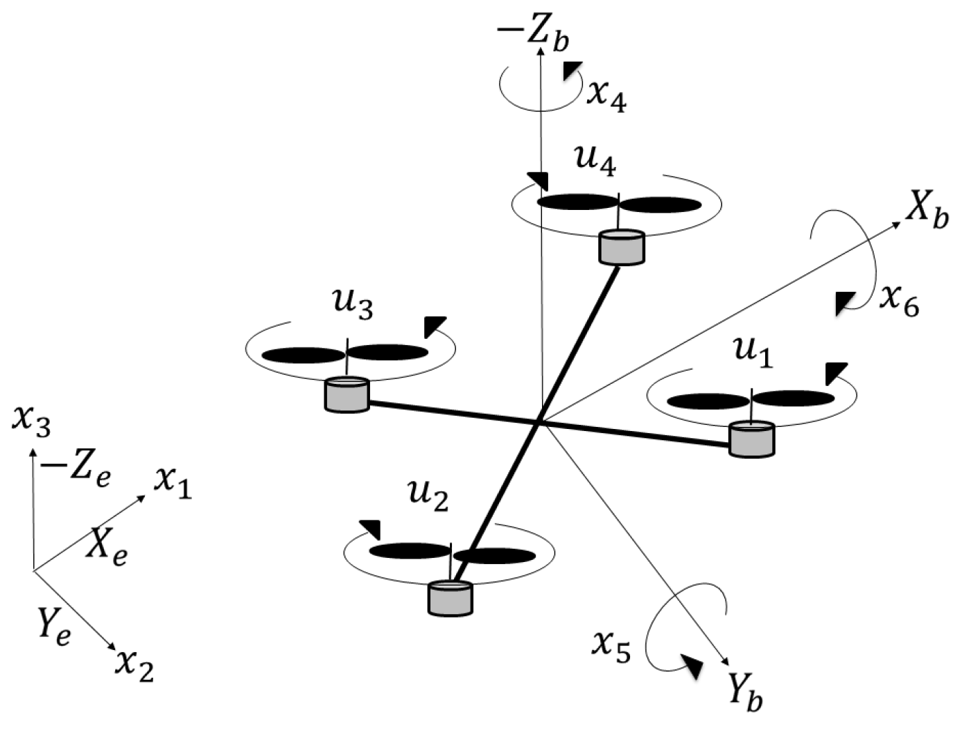
is the angular velocity of the i-th rotor. The schematics of this aircraft is given in
Figure 1. In aeronautics, the convention of measuring elevation or altitude through the negative part of the Z-axis is often a matter of mathematical and geometric consistency. The convention is motivated by the right-hand coordinate system commonly used in aviation and engineering: the X-axis points forward (along the longitudinal axis of the aircraft), the Y-axis points to the right (along the lateral axis), and the Z-axis points downward (along the vertical axis) [
25].
The dynamics of a quadcopter can be expressed as [
26,
27,
28,
29]:
where
,
, and
with
as the force responsible for throttle movement,
as the torque responsible for roll movement,
as the torque responsible for pitch movement, and
as the torque responsible for yaw movement, given by
Notice that , , and are the frequencies of rotors 1, 2, 3 and 4, respectively, i.e., they are the implicit control inputs and they are given in . The variables , and represent the linear displacements along the earth fixed axes , and , respectively, and they are in meters. On the other hand, the variables , and describe the angular displacements around the body axes , and , respectively, and they are in radians. The remaining state variables describe the linear and angular velocities, and they can be easily deduced from (7)-(24).
2.4. Simulink Support Package for Parrot Minidrones
The Simulink Support Package for Parrot Minidrones is a toolbox that enables users to design and deploy flight control algorithms for Parrot minidrones using Simulink. Users can wirelessly connect to the minidrones via Bluetooth and access their onboard sensors and camera. Users can also use additional tools such as Aerospace Blockset and Simulink Coder to enhance their simulations and code generation. The toolbox also includes an example that shows how to model and simulate the 6-DOF equations of motion for the minidrones [
30,
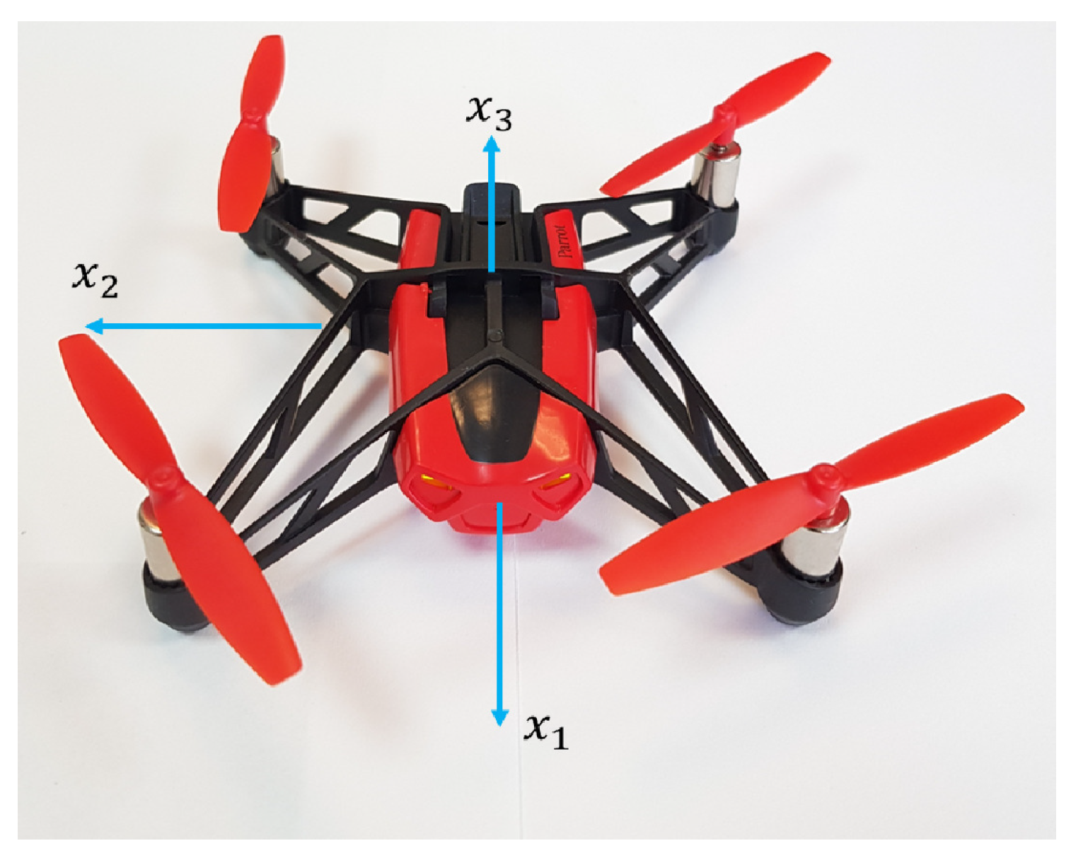
31]. In
Figure 2, the physical quadcopter simulated by the Simulink Support Package for Parrot Minidrones is depicted.
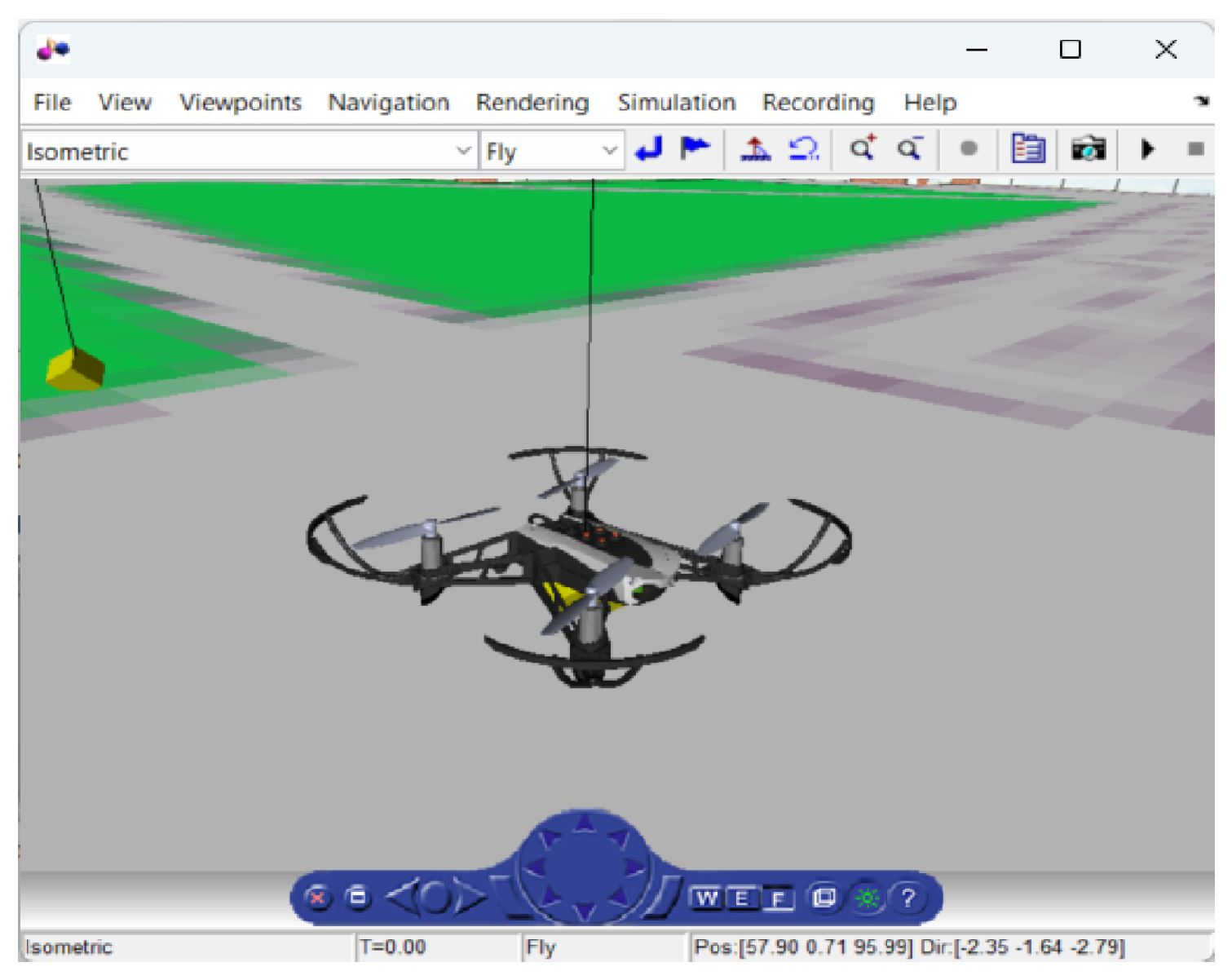
This package includes a Controller Project template designed as a framework for crafting a personalized controller or adapting it to specific needs. The template integrates a robust plant model simulation for both the Parrot Rolling Spider and Parrot Mambo drones. This simulation streamlines the evaluation of model outcomes before deployment, empowering users to scrutinize and refine their controller designs prior to applying them to the physical hardware. The template supports the modeling of six degrees of freedom (6-DOF) equations of motion, facilitating the simulation of aircraft behavior under diverse flight and environmental conditions.
Figure 3 depicts the VRML environment employed by the Simulink Package for Parrot Minidrones.
In the context of this study, the Simulink package’s simulation results are utilized to gather data for identifying the mathematical model of the quadcopter.
3. Identification of a High-Order Nonlinear Systems with Coupled Dynamics Using the Classical SINDY Algorithm
In this section, the Algorithm 1 is used to obtain the mathematical model of a quadcopter from the data generated by the Simulink Support Package for Parrot Minidrones.
For the sake of simplicity, throughout the remainder of this study, it is assumed that the Rolling Spider MiniDrone depicted in
Figure 2 can be effectively modeled using equations (7)-(19). In other words, the drone’s controls are considered to be
,
,
, and
, instead of
,
,
, and
. Adopting this perspective streamlines the required library of functions for SYNDY, specifically the matrix
. Despite this simplification, the resulting nonlinear system maintains sufficient complexity to reveal the limitations of the conventional SINDY approach. This underscores the advantages of the proposed modification, particularly in the identification of high-order nonlinear systems with coupled dynamics.
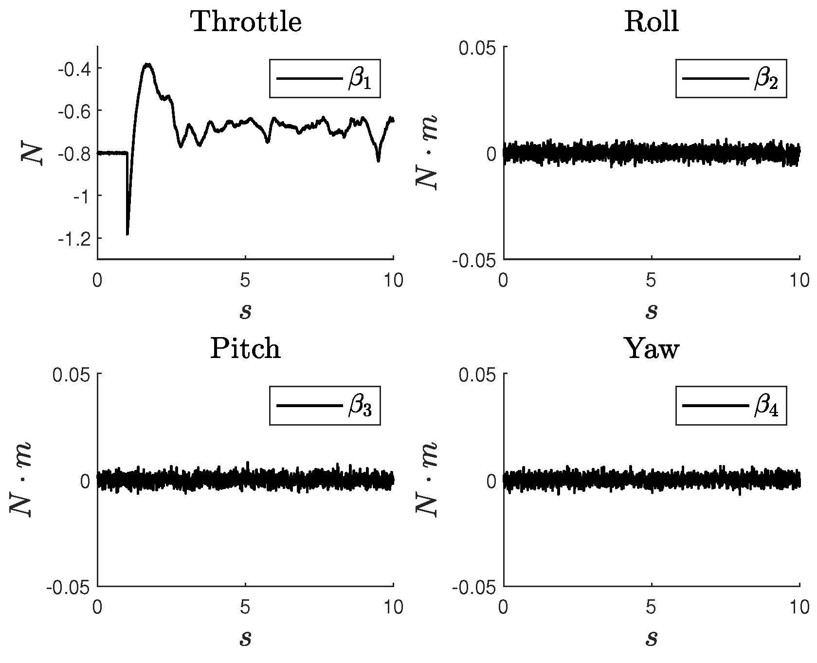
The Simulink Support Package for Parrot Minidrones is employed to simulate a 10-second flight sequence of the drone, with the samplig time
. Throughout this duration, the drone undergoes takeoff and ascends to an altitude of 1.5 meters. Meanwhile, the controls
,
,
, and
are subtly perturbed to excite all four independent degrees of freedom of the drone. These inputs are shown in
Figure 4.
During this simulated flight, the vectors are formed by reading the linear and angular displacements, linear and angular velocities, linear and angular accelerations, and controls. Clearly, .
So, to correctly formulate equation (
4), consider that the matrix
is:
while the matrix
is
with
,
,
,
,
,
,
,
,
,
,
,
,
,
,
,
, where as mentioned above,
. Thus, the unknown matrix
has a dimension of
.
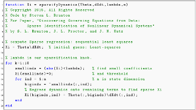
Now, the MATLAB code for the classical SINDY algorithm, with
,
,
, and
, is:
|
Listing 1: Matlab function for the classical SINDY |
 |
The matrix
produced is:
Notice that, in this case, the obtained identification is not sparse because every function considered in
appears from the seventh to the twelfth equation in the identified model, even when the parameter lambda is not very small, i.e.,
. But, even if one wants to suppose that the identified model is a possible representation of the nonlinear dynamics of the drone, the main drawback arises when it is realized that the obtained model is non-controllable, which must be incorrect, as the drone is, in fact, a controllable system [
32].
This example demonstrates that, in general, it is not sufficient to know the functions appearing in the model to be identified for SINDY to yield correct results. The following section addresses and mitigates this drawback.
4. Identification of a high-order nonlinear systems with coupled dynamics through the modified SINDY algorithm
4.1. GenesisXi algorithm
At this point, it is obvious that, in addition to knowing the functions that should appear in the model to be identified, it is important to know in which differential equation each of them should appear. This transforms the task of identifying the nonlinear model into a coefficient identification problem, which proves highly advantageous for a wide range of real-world nonlinear problems.
Therefore, the modification to the classical SINDY algorithm involves incorporating this additional information in a manner that the obtained result approaches the known models, specifically in this case, the models of the quadrotors.
To achieve this objective, it is necessary to formulate an initial matrix
wherein the positions of all candidate functions contained in
within the differential equations of the mathematical model are defined. To automate this process, the Algorithm 2 for obtaining the aforementioned matrix
is proposed.
|
Algorithm 2 GenesisXi algorithm |
Require: Data vector and n
Ensure: Initial matrix
- 1:
- 2:
fortoqdo
- 3:
- 4:
end for
|
The following is the description of the Algorithm 2:
- 1.
Given the vector , whose elements contain the number of the differential equation where the corresponding candidate function should be located, and n, which is the dimension of the nonlinear system to be estimated, then the matrix is set to zero. For this case, .
- 2.
The vector is traversed from its first element to the last using the index k, simultaneously placing a "1" at the position in the matrix .
The MATLAB code corresponding to Algorithm 2, with , is given in Listing 2.
|
Listing 2: MATLAB function for the GenesisXi algorithm |
 |
Thus, after applying Algorithm 2, and in accordance with (7)-(19), the resulting matrix
is:
Notice that the columns of
represent the differential equations in the nonlinear model, while the rows of
represent the candidate functions included in
. Thus, the matrix (
28) indicates that
appears in the ninth differential equation,
appears only in the second differential equation, and so forth.
4.2. Modified SINDY Algorithm
Now, the location of the candidate functions in the matrix is passed as a parameter to the modified SINDY function, as illustrated in the MATLAB code presented in Listing 3.
|
Listing 3: MATLAB function with modifications to classical SINDY |
 |
Roughly speaking, the modifications consist of removing the functions that wrongly appear in the differential equations after the first guess of the matrix in line 4. To achieve this, the MATLAB operator "" is applied to multiply each element of the matrix obtained in line 4 by the corresponding element of the matrix . In other words, is used as a template for the desired matrix . The remainder of the program follows exactly the structure of the classical SINDY function presented in Listing 1.
The matrix
obtained by applying the MATLAB function provided in Listing 3 to the data described in the previous section is:
This matrix corresponds to the sparse identification of the high-order nonlinear system with coupled dynamics, specifically, the drone. The identified nonlinear system is given by:
Notice that the gravity value in equation (38) is calculated as 4.725, which is 2.076 times smaller than 9.81. This implies that the entire equation is scaled by
. However, as per equations (14)-(16), when the identified model is analyzed at the equilibrium, i.e., when all linear and angular displacements, velocities, and accelerations are zero, and the mass
m is computed using equations (36), (37), and (38) multiplied by 2.076, it results in
,
, and
, respectively, which are very close to the nominal value found in literature of
[
30,
31].
Now, based on these equations, a linear stabilizer is designed. To achieve this, equations (30)-(41) are linearized at the equilibrium
, resulting in:
with
and
The stabilizer
is obtained using the Linear Quadratic Regulator (LQR) approach, which combines the control energy and the state deviations in the cost function of the form:
where
Q and
R are positive definite matrices determining the compromise between minimizing the state deviations and the control energy [
32]. In this case,
, and
. Thus, with matrices
A,
B,
Q, and
R as above, the gain
K is computed using the MATLAB function
, resulting in:
Then, the stabilizer
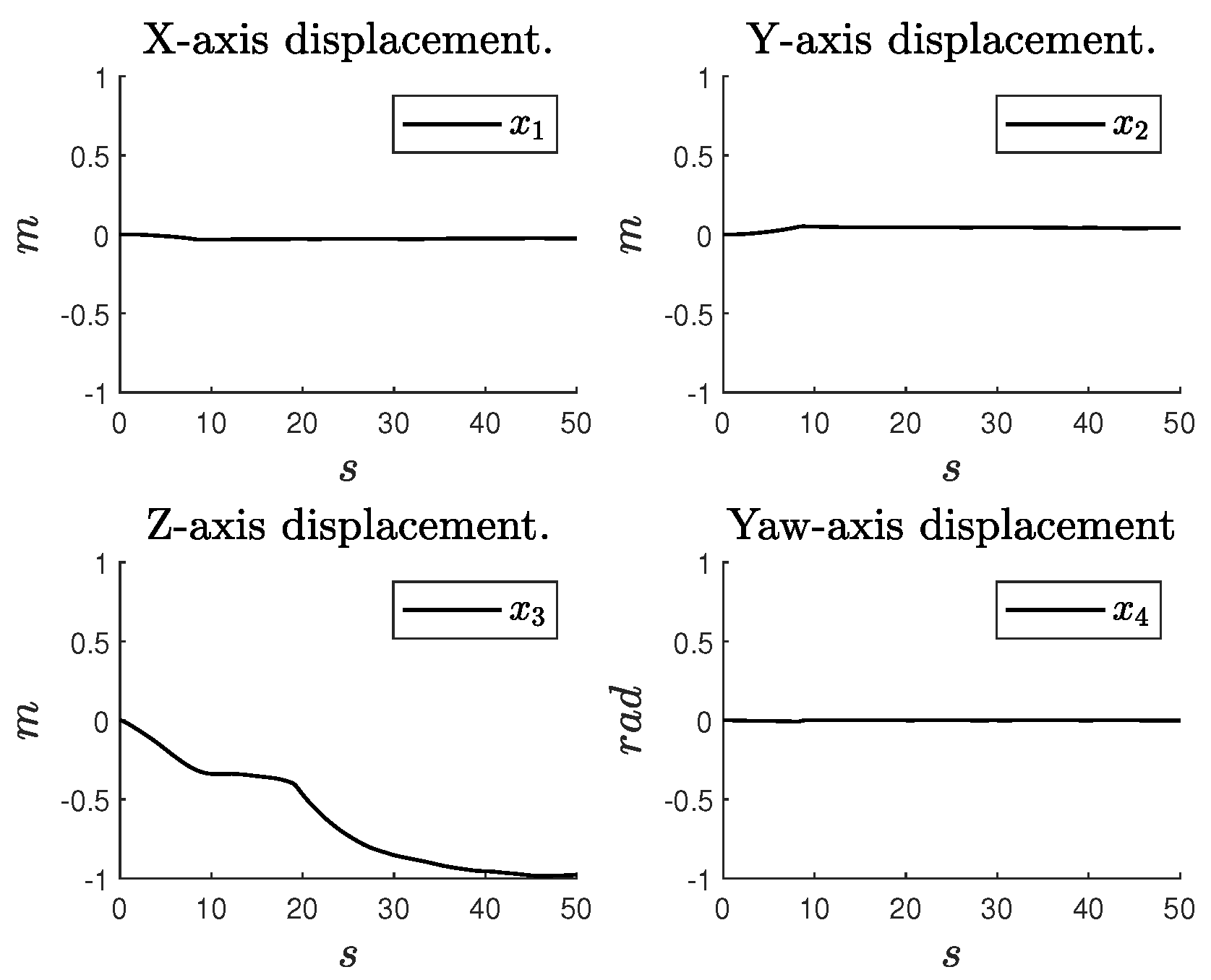
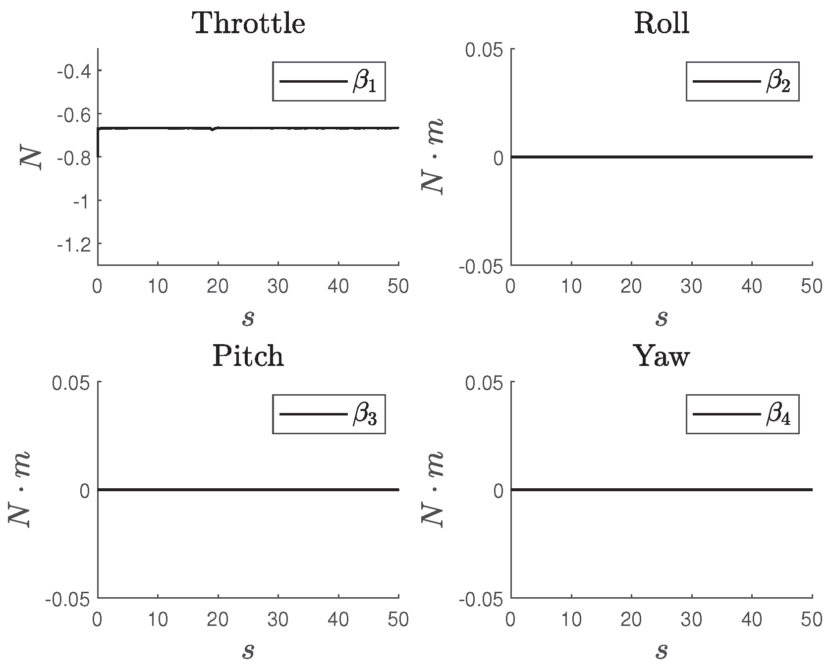
is applied to the nonlinear model within the Simulink Support Package for Parrot Minidrones to assess the effectiveness of the identified model. In this example, the quadcopter reaches an altitude of 1m using the linear stabilizer. The numerical results are presented in
Figure 5 and
Figure 6.
Figure 5 illustrates the drone’s response to the linear stabilizer, while
Figure 6 displays the corresponding input signals.
Please note that the goal of this work is not to design sophisticated controllers aiming for complex behaviors in the drone. Instead, the primary contribution of this work is to introduce an alternative method for obtaining the mathematical model of high-order nonlinear system with coupled dynamics based on real-time measured data.
5. Discussion
- 1
In the specific case study, the outcomes achieved through the classical SINDY algorithm do not align with physics-based identification. Moreover, they do not qualify as sparse identification, as all candidate functions are present in the matrix .
- 2
Based on the knowledge of the structure of the complex system to be identified, a more precise algorithm has been introduced without a significant increase in computational cost.
- 3
Although the identified model appears to have significant differences from the related model found in the literature, it enables the design of a controller capable of stabilizing the original high-order nonlinear system with coupled dynamics. This, in turn, demonstrates its notable approximation degree.
- 4
The primary drawback of the proposed approach is that the identification problem transforms into a coefficient identification task. Nevertheless, in many real-world applications, this outcome may still be appealing because, in numerous cases, it is impossible to precisely determine the coefficients of a specific system, even when the structure of its mathematical model is available.
6. Conclusions
This work introduces a modification to the classical SINDY algorithm, enabling the identification of the mathematical model for high-order nonlinear systems with coupled dynamics. The computational cost of the modification is negligible compared to the advantages gained. However, a drawback is the requirement to know the structure of the nonlinear model to generate the template for placing the nonlinear functions in the appropriate differential equations. The proposal was validated by applying a linear controller designed based on the identified model to the real system.
Author Contributions
Conceptualization, R. D. V.-S. and J. A. M.-C.; formal analysis, R. P.-G., R. D. V.-S., J. O. E.-A. and R. T.-H.; investigation, J. O. E.-A., R. T.-H. and J.A.M.-C.; methodology, J. O. E.-A., R. T.-H. and J.A.M.-C.; project administration, J. A. M.-C.; writing—original draft, J. A. M.-C.; writing— review and editing, R.D.V.-S. J.O.E.-A., R.P.-G., R.T.-H. and J. A. M.-C. All authors have read and approved this version of the manuscript.
Funding
This research received no external funding.
Data Availability Statement
Data are contained within the article.
Acknowledgments
The authors gratefully acknowledge the partial support provided for this research by the Consejo Nacional de Humanidades Ciencias y Tecnologías (CONAHCYT) through the SNI (Sistema Nacional de Investigadores) scholarship. Additionally, the Instituto Politécnico Nacional contributed to this work through research projects 20230023 and 20240025, as well as by providing scholarships under the programs EDI (Estímulo al Desempeño de los Investigadores), COFAA (Comisión de Operación y Fomento de Actividades Académicas), and BEIFI (Beca de Estímulo Institucional de Formación de Investigadores).
Conflicts of Interest
The authors declare no conflict of interest.
References
- Editorial. The rise of data-driven modelling. Nature Reviews Physics 2021, 3, 845–855. [Google Scholar] [CrossRef]
- Moghadas, S.M.; Jaberi-Douraki, M. Mathematical Modelling: A Graduate Textbook; John Wiley & Sons, Inc.: River Street, Hoboken, NJ, 2019. [Google Scholar]
- Montáns, F.J.; Chinesta, F.; Gómez-Bombarelli, R.; Kutz, J.N. Data-driven modeling and learning in science and engineering. Comptes Rendus Mécanique 2019, 347, 845–855. [Google Scholar] [CrossRef]
- Devo, A.; Mao, J.; Costante, G.; Loianno, G. Autonomous Single-Image Drone Exploration With Deep Reinforcement Learning and Mixed Reality. IEEE Robotics and Automation Letters 2022, 7, 5031–5038. [Google Scholar] [CrossRef]
- Schmidt, M.; Lipson, H. Distilling Free-Form Natural Laws from Experimental Data. Science 2009, 324, 81–85. [Google Scholar] [CrossRef] [PubMed]
- Peña-García, R.; Velázquez-Sánchez, R.; Gómez-Daza-Argumedo, C.; Escobedo-Alva, J.; Tapia-Herrera, R.; Meda-Campaña, J. Physics-Based Aircraft Dynamics Identification Using Genetic Algorithms. Aerospace 2024, 11, 1–18. [Google Scholar] [CrossRef]
- Haring, M.; Grøtli, E.I.; Riemer-Sørensen, S.; Seel, K.; Hanssen, K.G. A Levenberg-Marquardt Algorithm for Sparse Identification of Dynamical Systems. IEEE Transactions on Neural Networks and Learning Systems 2022, pp. 1–14. [CrossRef]
- Tibshirani, R. Regression Shrinkage and Selection Via the Lasso. Journal of the Royal Statistical Society: Series B (Methodological) 1996, 58, 267–288. [Google Scholar] [CrossRef]
- Brunton, S.L.; Proctor, J.L.; Kutz, J.N. Discovering governing equations from data by sparse identification of nonlinear dynamical systems. Proceedings of the National Academy of Sciences - Applied Mathematics 2016, 113, 3932–3937. [Google Scholar] [CrossRef] [PubMed]
- Hansen, P.C.; Pereyra, V.; Scherer, G. Least Squares Data Fitting with Applications; Johns Hopkins University Press: Baltimore, 2013. [Google Scholar]
- Bertrand, Q.; Klopfenstein, Q.; Blondel, M.; Vaiter, S.; Gramfort, A.; Salmon, J. Implicit differentiation of Lasso-type models for hyperparameter optimization. In Proceedings of the Proceedings of the 37th International Conference on Machine Learning; III, H.D.; Singh, A., Eds., Virtual Event, 13–18 Jul 2020; Vol. 119, Proceedings of Machine Learning Research, pp. 810–821.
- Brunton, S.L.; Kutz, J.N. Data-Driven Science and Engineering: Machine Learning, Dynamical Systems, and Control; Cambridge University Press: Cambridge, MA, 2019. [Google Scholar] [CrossRef]
- Brunton, S.L.; Proctor, J.L.; Kutz, J.N. Disco2vering governing equations from data by sparse identification of nonlinear dynamical systems. Proceedings of the National Academy os Sciences of the United States of America 2018, 113, 3932–3937. [Google Scholar] [CrossRef]
- Burrage, P.M.; Weerasinghe, H.N.; Burrage, K. Using a library of chemical reactions to fit systems of ordinary differential equations to agent-based models: a machine learning approach. Numerical Algorithms 2024. [Google Scholar] [CrossRef]
- Cao, R.; Lu, Y.; He, Z. System identification method based on interpretable machine learning for unknown aircraft dynamics. Aerospace Science and Technology 2022, 126, 107593. [Google Scholar] [CrossRef]
- Callaham, J.L.; Brunton, S.L.; Loiseau, J.C. On the role of nonlinear correlations in reduced-order modelling. Journal of Fluid Mechanics 2022, 938. [Google Scholar] [CrossRef]
- Sargsyan, S.; Brunton, S.L.; Kutz, J.N. Nonlinear model reduction for dynamical systems using sparse sensor locations from learned libraries. Phys. Rev. E 2015, 92, 033304. [Google Scholar] [CrossRef] [PubMed]
- Loiseau, J.C.; Brunton, S.L. Constrained sparse Galerkin regression. Journal of Fluid Mechanics 2018, 838, 42–67. [Google Scholar] [CrossRef]
- J.-C. Loiseau, S.L.B.; Noack, B.R., 9 From the POD-Galerkin method to sparse manifold models. In Volume 3 Applications; De Gruyter: Berlin, Boston, 2021; pp. 279–320. [CrossRef]
- Zavialov, V.; Lobok, O.; Mysiura, T.; Popova, N.; Chornyi, V.; Pohorilyi, T. Identification of unknown parameters of the dynamic model of mass transfer. Mathematical Modelling and Analysis 2023, 459–468. [Google Scholar] [CrossRef]
- Hritonenko, N.; Satsky, C.; Yatsenko, Y. Integral model of COVID-19 spread and mitigation in UK: identification of transmission rate. Mathematical Modelling and Analysis 2022, 573–589. [Google Scholar] [CrossRef]
- Dodge, Y. The Concise Encyclopedia of Statistics - Least-Squares Method; Springer: New York, NY, 2008. [Google Scholar] [CrossRef]
- Margalit, D.; Rabinoff, J. Interactive linear algebra; Georgia Institute of Technology: Atlanta, GA, 2019. [Google Scholar]
- D. C. Lay, S.R.L.; McDonald, J.J. Linear algebra and its applications; Pearson: New York, NY, 2016.
- Phillips, W.F. Mechanics of Flight; John Wiley and Sons, Inc.: New Jersey, 1980. [Google Scholar]
- Meda-Campaña, J.A.; Torres-Cruz, R.E.; Rojas-Ruiz, A.J.; Tapia-Herrera, R.; Hernández-Cortés, T.; Páramo-Carranza, L.A. The Output Regulation and the Kalman Filter as the Signal Generator. IEEE Access 2023, 11, 90825–90838. [Google Scholar] [CrossRef]
- Jennie, Y.; Fathurrahman, A.; Arifianto, O.; Sasongko, R. Mathematical modelling and simulation of a quadrotor unmanned aerial vehicle with automatic altitude and speed control. AIP Conference Proceedings 2020, 2226, 020011. [Google Scholar]
- Collazos Morales, C.A.; Ospina, J.P.; Sánchez, J.F.; Caro-Ruiz, C.; Grisales, V.H.; Ariza-Colpas, P.; De-la Hoz-Franco, E.; González, R.E. Mathematical Modelling and Identification of a Quadrotor. In Proceedings of the International Conference on Computational Science and Its Applications. Springer; 2020; pp. 261–275. [Google Scholar]
- Mohamed, A.; Elsayed, M.; Elshafei, M. A Comparative Study Between a Classical and Optimal Control of a Quadrotor UAV. arXiv 2020, arXiv:2009.13175 2020. [Google Scholar]
- MathWorks. Parrot Minidrones Support from Simulink, 2023. https://www.mathworks.com/hardware-support/parrot-minidrones.html.
- MathWorks. Simulink Support Package for Parrot Minidrones Documentation, 2023. https://www.mathworks.com/help/supportpkg/parrot/.
- Kailath, T. Linear Systems; Prentice–Hall, Inc.: New Jersey, 1980. [Google Scholar]
|
Disclaimer/Publisher’s Note: The statements, opinions and data contained in all publications are solely those of the individual author(s) and contributor(s) and not of MDPI and/or the editor(s). MDPI and/or the editor(s) disclaim responsibility for any injury to people or property resulting from any ideas, methods, instructions or products referred to in the content. |
© 2024 by the authors. Licensee MDPI, Basel, Switzerland. This article is an open access article distributed under the terms and conditions of the Creative Commons Attribution (CC BY) license (https://creativecommons.org/licenses/by/4.0/).
