
Submitted:
13 March 2024
Posted:
13 March 2024
You are already at the latest version
Abstract
Classically the walk in biped robotics was obtained controlling balance during the whole step, i.e. guaranteeing that the pressure point under the soles always stayed in the polygon of the supporting feet. However, this assumed that the feet were able to transfer torque to the ground during the whole gait cycle. In spite of the fact that the amount of transferrable torque in the feet-ground contact is limited, it is possible only during some phases of the step, and the overall process is energetically inefficient. On the other side, starting from the passive motion of the rimless wheel falling on an inclined surface, and ending to the inverted pendulum with a compass, balance in the whole was proven in spite of dynamical instability inside each step. Along this line results of Foot Placement Estimation (FPE) in 2-D and 3-D showed how energy efficient walk was possible, emulating the human walk with a free fall on the swing foot and energy restitution at the foot collision with the ground for the next step. This model assumes pointy feet, so without torque transfer to the ground. In the realm of FPE, in previous papers the present author adopted the 3-D inverted pendulum in polar coordinates (Spherical Inverted Pendulum - SIP) to introduce omnidirectional walks with arbitrarily changing characteristics. No torque control was used during the step, i.e the pendulum was always in free fall at each step, the only control actions were at the beginning of the next step. These actions are: the change of angular velocities at the start of a new step, with respect to those given after the collision (emulating the torque action in the brief double stance period), to recover for the losses, and the preparation of the position in the frontal and sagittal planes of the swing foot for the next collision. The present paper improves this paradigm, proposing a general model to account for all characteristics of the biped and of the gait, with adding a minimum of dynamical complexity with respect to the SIP. This model allows, not only to walk omnidirectionally on a flat surface, but also to go up and down staircases.
Keywords:
Humanoid and Bipedal Locomotion
; Legged Robots
; Passive Walking
; Foot Placement Estimation
; Spherical Inverted Pendulum
1. Introduction
Originally balance in the gait of biped robots was achieved controlling that the pressure center under the soles stayed in the supporting polygon of the feet during the whole step. The terminology of zero moment point (ZMP) was introduced [1].
In that period, fundamental was the work of Kajita [2,3] that introduced, using the inverted pendulum and imposing a constant hight of the center of gravity (COG) the linearized inverted pendulum model (LIPM). He showed with the LIPM that in a flat surface the trajectories of the pressure point in the frontal and sagittal planes were decoupled, and a simple linear relationship linked the ZMP with the projection of the COG position and COG acceleration on the two horizontal axes ().
In order to be able to transfer the needed torque to the ground the feet were maintained flat, with a walk of the robot unrealistic and energetically inefficient.
In a second phase the rotation of the feet with respect to the ground was introduced. The control, during the gait, was divided in phases, where during one of the phases, when on the tip of the foot, the control was underactuated [4,5].
In reality, human-like gait, with its mix of fully actuated and underactuated phases (where walking during one of the phases is a “controlled falling”) is more complex [6]. Push recovery, walking on rough terrain, and agile footstep control are active research topics [7].
On a completely different line of approach, in the realm of passive walkers and of hybrid zero dynamics [8,9,10], starting from the passive motion of the rimless wheel falling on an inclined surface, and ending to the inverted pendulum with a compass, stability of the gait in the whole was proven in spite of dynamical instability inside each step.
The model used was the spherical inverted pendulum (SIP) in polar coordinate system, i.e., the 2 DOFs of the pendulum are the rotation around the vertical axis, and one of the horizontal axes [11,12]. With the SIP model the problem of gait is intertwined with the estimation in 3-D of the swing foot placement at the collision with the ground (FPE) [13,14,15,16,17]. This has been obtained using energy relationships, observing that the total energy, and the partial derivative of the kinetic energy with respect to the rotational velocity (i.e., the angular momentum) along the vertical axis are constant during a step.
In a first paper [18] this author using the SIP model with 2 DOFs achieved an omnidirectional walk without any torque control, but simply, exploiting the fall of the pendulum and the anelastic restitution of the collision of the swing foot with the ground. At each step, before the next, the initial rotational velocities after the collision were properly increased to cope with the losses, and the angles of the swing leg were set to define the position of the next foot placement for balance and for navigation. So doing, the direction, the speed of the walk, the length of the steps where controlled.
To overcome certain limitations, expecially the COG sway in the frontal plane, in a second paper [19] the SIP model, always with 2 DOFs, was extended adding a pelvis width and introducing the distance between the hips of the two legs.
In this paper, the model of this represention is, one more time, extended with 3 rotational DOFs, where pelvis width, distance of the supporing feet and sway of COG in the frontal plane, can be controlled. Moreover, to allow to go up and down staircases one further prismatic DOF is added to modify the length of the supporting leg during the step.
With respect to the classical gait control the problem has here been reversed. Instead of two phases of the step (double and single stance): based on controlling foot torques during double support, and the first part of single support when the foot is flat, and handling underactuated control when the robot is on the foot’s tip, the whole step is always in free fall, and the changes of the velocities, with respect to the values given by the collision, before the next step are virtually the results, of a (impulsive) torque action during the double stance phase, that here has time period zero.
In Section 2 the model is presented. The gait control is reviewed from previous papers [18,19], by addding some new aspect, in Section 3. Examples of going up and down the staircases, intertwined with the navigation is presented in Section 4. The Foot placement estimation for ending in equilibrium a walk is discussed in Section 5. Conclusions and forecast of further extensions are in Section 6. Appendices report from [18], in Appendix A the Kane’s method used for the simulation, and in Appendix B the simbolic formulas for FPE on the balanced arrival.
2. The Spherical Inverted Pendulum with Pelvis Width and Changing Length of the Supporting Leg
The model adopted in this paper adds, with respect to the original SIP, in the compass, the width of the pelvis and the distance between the hips of the two legs. It has 3 rotational DOFs, instead of 2, for walking on a flat horizontal surface, and one more prismatic DOF on the supporting leg for going up and down staircases. In fact the control of the only three rotational DOFs is not enough in this case. Its kinematics is represented in Figure 1a. The axes of the local frames of the segments have a similar disposition as the inertial frame N. The multibody is composed of four segments: the supporting leg, composed of two parts connected with a prismatic link, the flying leg and the pelvis. The two legs are massless. Only the pelvis, representing also the upper body of the biped, has a mass and an inertia.The prismatic link in the supporting leg, , is controlled in position by a force , through a spring and a damper (Figure 1b), using a step reference when climbing and descending staircases, and it is connected to the pelvis through the joints with angles and . These angles are constant during a step and are set, at the beginning of each step, to maintain the orientation of the pelvis in the hybrid model at the pivot switching. The 3 DOFs offered to the SIP by the supporting leg are represented by the joints of angles , and . They define, in body coordinate 3-2-1 (ZYX), the orientation of the leg’s frame. The length of the swing leg, , is set and maintained according to the height of the steps of the staircase (shorter when climbing, at the full length when descending). The leg is connected to the pelvis through the joints of angles and . Also these angles are constant during a step and are set, at each step, to define the future position of the swing foot at the ground collision. The characterist points of the model are the two feet ( and ), the two hips ( and ) and the COG. The two legs have identical length when walking on a flat horizontal surface, while the supporting leg has a transition from an initial value, identical to the swing leg length, to a final value during a step going up or down a staircase.
A parameter, called here , assuming values , accounts for right and left supporting foot in the hybrid simulation, otherwise the models are identical in the two cases.
When the prismatic joint is locked, the model has 3 DOF plus 3 positions of the supporting foot . The dynamics is of order 12 with configuration variables , and corresponding motion variables . However, a non-holonomic constraint imposes a fixed position of the pivot foot () during the swing. When moving on a staircase, the prismatic joint adds 2 degrees to the dynamics: position l with velocity contributing to the length of the supporing leg (i.e., and ). The non-holonomic constraint is released, only, at the collision of the swing foot with the ground to define, through anelastic restitution, the initial motion values for the next step , and in the case of . For all the details of the dynamics refer to the father paper [18] and to the appendices Appendix A and Appendix B.
Switching Supporting Foot after Ground Collision
The touch down is given when the vertical position of foot reaches the ground, and the anelastic collision defines , , and . The switching of pivot feet is computed in two steps, through non-linear least squares:
- by equating the direction cosine matrix of the swing leg frame at the touch down to a new frame expressed by orientation angles in body coordinate 3-2-1 (ZYX), and assigning these angles, as initial values, to , and to the new supporting leg;
- computing and in order to guarantee the constancy of the direction of the y axis of the pelvis local frame before and after the switching of the pivot foot and resetting to zero the previous rotation along this axis.
3. The Gait
In the new paradigm the control of the gait of the hybrid system is performed by assigning initial values to , , , () and to and at the beginning of each step. In previous works [18,19] the model with 2 DOFs behaved as a 3-D inverted pendulum and, in particular [19], the y axis of the pelvis always remained horizontal during the whole step. Global stability was assured assigning any reasonable initial values of , . In the present case the model with 3 DOF adds a rotation of the pelvis along its x axis. Global stability can be achieved only if the rotation along the x axis is regulated in cloed loop by controlling al the beginning of each step the initial value of (responsible for the motion) from the samples after the previous collision. This was achieved alternatively with a sampled data PID feedback or a self tuning regulator [20]. The self tuning regulator, in particular, was adopted to minimize the variance of the oscillations of .
The expressions of section 5 of [18], properly modified in Appendix B, for FPE, at difference of [13,14,15,16], are not directly used here at each step; they are exploited to impose a stop at the end of the walk.
In closed loop, a perturbation to is chosen to control the desired step length, to to control the desired distance, along the y axis, of the supporting foot, the COG sway and also the offset with respect to the desired baseline in the navigation (as usual, the real time, sampled data, control is achieved by assigning at the beginning of every step the initial values of the motion variables and of the flying leg angles for the next step, based on the final angles and position values of the flying foot at touchdown of the previous step.). The gait is initiated giving an initial condition to , or, simply, from a standing up balance by leaving the pendulum to fall forward. Each step is concluded when the swing foot touches the ground (the vertical coordinate of point becomes zero, Equation (A22)). From the impact Equation (A20) the new motion variables are determined (consequently the kinetic energy results, also), and from Equations (A24) and (A25) the starting values of and for a new step are computed. The gait is maintained by increasing at each step and , resulting after impact, to compensate for the reduction of kinetic energy: the first to guarantee the desired gait cadence, the latter to correct the direction of walk. Vice versa, is controlled in closed loop directly from to maintain horizontality and minimize the oscillations of the pelvis around the x axis.
In the present model the two legs have not mass and inertia. So, the motions of the angles and are istantaneous and energy free. In a horizontal ground the only energy contribution to mantain the walk is given by proper impulsive forces and torques just after the impact to modify the velocities , and resulting from the impact. This emulates, in a real walk, the contribution given by the biped in the brief double support phase and in the period of single support when the foot is flat and able to transfer torques. On a staircase, the length of the supporting leg has to be controlled during the whole step and the energy related to its motion has to be added.
Six control variables are identified to control six objectives of the walk: and variance of around the x axis of the pelvis, the , , , y with respect to the baseline of walk, and (Even if interacting each other, each of the six variables predominantly controls one of the six objectives). After each impact, at the start of step k they are
where u assumes the values according to the right or left foot support.
It must be noted that no periodic reference is tracked. The whole gait style (cadence, length of the step, offset with respect to the baseline of walk-through a side shuffle, spacing between the two feet and direction) can be changed at each step.
The next Figure 2 and Figure 3 show a sample of a typical rectilinear walk on an horizontal ground. In Figure 2b the ZMP is estimated using the Kajita’s formulas.
The two Figure 4, vice versa, show the total energy and the angular momentum about the vertical axis during the ascending of a staircase.
As it can be seen in Figure 4 the total energy si not constant in the first period of the step time, due to the change of length of the supporting leg. In this case the properties of a pure ballistic motion are lost because an energy is injected into the system during the step.
4. Going Up and Down the Staircases
The strategy of Equation (1) adds to the initial conditions of and the values needed to compensate the reduction of rotational energy due to the impact, but not to move the pendulum in a vertical direction. For this, the prismatic link has been added. If going up the staircase (Figure 5), the flying leg is shortened, with respect to the full length, of the value of the stair’s step. This same length will be the initial value of the next supporting leg, that during the first period of the step will have a transition to full length. Vice versa, if going down (Figure 5) , the flying leg is at full length, and the supporting leg will be shortened, during the step, from the full length to a value corresponding to the heigth of the stair’s step. In the paper this transition is achieved with a force control of the prismatic link tracking with a PD filter a step reference. The values of the filter allow to model, also, the rigidity and damping of the knee.
Two examples are presented. The first (Figure 6a) embeds, also, a navigation control on a spiral staircase with a ray of 5 meters. The second (Figure 6b) shows the and going up and down a rectilinear staircase. In the second example let note a perturbation in the sway on the frontal plane when the direction is changed, but it is quickly recovered.
5. Foot Placement Estimation
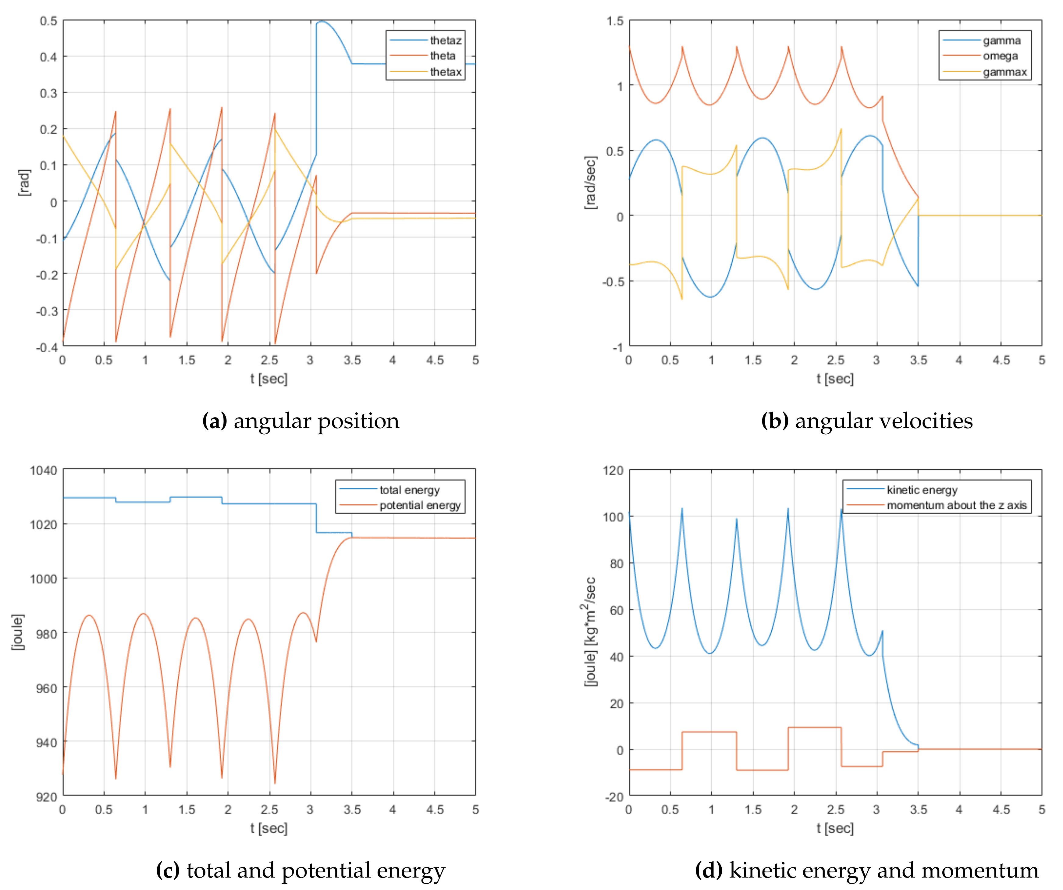
The formulas of the appendices Appendix A and Appendix B for the foot placement estimation are used for stopping in equilibrium at the end of the walk.
On a staircase the computation is performed when the transient on l has been concluded () and in the formulas the transient is ignored. However, for simplicity an example on horizontal ground is shown in Figure 7.
Obviously, reaching the quasi-equilibrium position after the last contact, given the pelvis width, the biped has to move in double support. In the example it happens at instant 3.5 sec. At this instant let note the non perfect zeroing of the kinetic energy and momentum (hence the angular velocities). This is due to the fact that, for simplicy, the FPE computation is performed at the maximum hight of the COG as a function of and , but this value in reality is not reached.
6. Conclusions
With this model of the biped the SIP has been extended with a minimum increase of the dynamics. It is possible to control in real time all parameters of the gait with an omni-directional walk on the flat ground or on the staircases. However, the purely ballistic motion of the pendulum is lost. Then, during the walking step the constancy of the total energy, on which is based the FPE, is no longer true. Nevertheless, FPE can, still, be evaluated performing the computations after the transient, setting in the formulas and adopting two models before and after the last contact with the length of the supporting leg at its initial and final value, respectively.
Two extensions of the present approach are envisaged:
Funding
This research received no external funding.
Conflicts of Interest
The author declares no conflicts of interest.
Abbreviations
The following abbreviations are used in this manuscript:
| FPE | Foot Placement Estimation |
| SIP | Spherical Inverted Pendulum |
| ZMP | Zero Moment Point |
| COG | Center of Gravity |
| LIPM | Linear Inverted Pendulum |
| DOF | Degree of Freedom |
Appendix A. The Kane’s Method and Autolev
In this work, the so-called Kane’s method [23] was adopted to model the spherical inverted pendulum. This method is particularly interesting in this case because it is equally applicable to either holonomic and non-holonomic systems and, for non-holonomic systems, without the need to introduce Lagrangian multipliers. Moreover, prof. Kane of Stanford, along the theory, has, also, developed a symbolic manipulation software environment, called Autolev (now MotionGenesis) [24], to support his method and to generate fragments of very efficient code of all needed mathematical expressions that are enbedded into the dynamical simulator and into the nonlinear numerical solvers needed for handling the switching of the model in the hybrid simulation at the collision of the swing foot with the ground and for computing the FPE.
Briefly, the main contribution of the Kane’s method is that, through the concepts of motion variables (later called generalized speeds), the vectors of partial velocities and partial angular velocities, generalized active forces and generalized inertia forces, the dynamical equations are automatically determined, enabling forces and torques with no influence on the dynamics to be eliminated early in the analysis. Early elimination of these noncontributing forces and torques greatly simplifies the mathematics and enables problems with greater complexity to be handled.
Appendix A.1. Generalized Coordinates and Speeds
A multi-body system, which possesses n degrees of freedom, is represented by a state with a n-dimensional vector of configuration variables (generalized coordinates) and an identical dimension vector of generalized speeds called also motion variables, that could be any nonsingular combination of the time derivatives of the generalized coordinates that describe the configuration of a system. These are the kinematical differential equations:
may be in general nonlinear in the configuration variables so that the equations of motion can take on a particularly compact (and thus computationally efficient) form with the effective use of generalized speeds.
Appendix A.2. Partial Velocities and Angular Velocities
Partial velocities of each point (partial angular velocity of each body) are the n three-dimensional vectors expressing the velocities of that point (angular velocity of that body) as a linear combination of the generalized speeds. Let be the translational velocity of a point B and the rotational velocity of a body P with respect to the inertial reference frame, then
where and are the rth partial velocity and partial angular velocity of B and P, respectively.
Appendix A.3. Generalized Active and Inertia Forces
The n generalized forces acting on a system are constructed by the scalar product (projection) of all contributing forces and torques on the partial velocities and partial angular velocities of the points and bodies they are applied to.
Let us consider a system composed by N bodies , where the torque , and force applied to a point of are the equivalent resultant (“replacement” [23]) of all active forces and torques applied to . Then
is the rth generalized active force acting on and
the rth generalized active force acting on the whole system. Identically for the inertia forces, indicated as .
The dynamical equations for an n degree of freedom system are formed out from generalized active and inertial forces
These are known as Kane’s dynamical equations.
They result in a n-dimensional system of second order differential equations ( order state variable representation) on generalized coordinates and speeds
where the parameter definitions are similar but not identical of the classical Lagrangian form and more efficient computationally [25].
Appendix A.4. Non-Holonomic Constraints
When m constraints on the motion variables are added to the model, only generalized speeds are independents.The system is, then, called a non-holonomic system. The non-holonomic constraints are expressed as a set of m linear relationships between dependent and independent generalized speeds of the type
with . In this case, selected the independent speeds, the Kane’s method immediately offers the minimal order state variable representation from
where Kane calls and non-holonomic generalized active and inertial forces, while the remaining m original redundant equations resolve themselves in the expressions of the m reaction forces/torques returned by the constraints. Because the Kane’s method is fundamentally based on the projection of forces on a tangent space on which the system dynamics are constrained to evolve, spanned by the partial velocities, reaction forces/torques result from the projection on its null-space.
Moreover, it is always possible to handle an holonomic (configuration) constraint as if it is non-holonomic, that is, to treat it as a motion constraint. This is particularly advantageous to represents the spherical inverted pendulum with a compass during a step, where in the first phase non-holonomic constrains allow pivoting on the supporting leg, and in the second phase, releasing the non-holonomic constraints the impact of the swing leg with the ground can be represented.
Appendix A.5. Unilateral Constraints and Collision
As a consequence of switching between different non-holonomic models during gait, unilateral constraints and collisions cannot be ignored.
Clearly, adopting non-holonomic dynamics assuming points of the feet fixed to the ground is valid for bilateral constraints (ignoring eventual detachment from the ground and slipping). In the approaches known as hybrid complementarity dynamical systems based on forward dynamics [26] the necessary conditions for satisfying unilateral constraints are directly embedded into the model. Vice versa, a minimalistic view is adopted here, noting that in a physiological gait, normally, bilateral constraints on the feet are not assumed to be violated. Hence, we design a priori walking strategies and we test through the simulator that this effectively occurs, by monitoring, a posteriori, reaction forces for the conditions:
and
Obviously, the control we propose cannot adapt itself to pathological conditions, such as a slipping surface.
For the second point, mechanics of the collision of the swing foot to the ground has to be considered, when switching to the next step causes the transfer of final conditions of the generalized speeds of one phase to the initial conditions of the successive. With reasonable assumptions of non-slipping and anelastic restitution the reaction impulsive force at the impact point B and the initial conditions of the generalized speeds for the new phase can be computed. Also for this aspect, Autolev offers all needed mechanical expressions.
The following analysis is based on two concepts: generalized impulse and generalized momentum [23,27]. Indicate, as usual, with the r-th component of the partial velocity vectors of the point B (the swing foot), the generalized impulse at the point B at the contact with the ground at instant is defined as the scalar product of the integral of the reaction impulsive force in the time interval with the corresponding partial velocities
the generalized momentum is defined as the partial derivative of the kinetic energy K with respect to the r-th generalized speed
then, Kane proves that
Indicate the matrices
of vectors of partial velocities, and of partial derivatives of with respect to the generalized speeds, and the vectors
of generalized impulses, of generalized speeds, of the velocity of point B and of generalized momenta, respectively.
Appendix B. FPE-the Balance Point at the Arrival
Before the impact the motion variables have value and after . is assumed zero. The total energy, T, and the projection on the vertical axis of the angular momentum, , are constant before and after the impact, however, they have a reduction during the impact. The constancy of the total energy is not true in the case of motion of the supporting leg, as the total energy has a transient in the first period. So, the computations are performed after the transient.
Let say that at time the state variables assume the values , the total energy , and the momentum on the vertical axis (these last two values are the same, also, at the unknown instant of the impact ). This gives the first equation, linking all state variables at the pre-impact.
At the impact the swing foot touches the ground. The vertical coordinate of offers the second equation, linking the pre-impact angle to and
This, also, offers the future new position of the supporting foot, let say and The constant momentum offers the third equation, linking to the other pre-impact motion variable
Switching the pivot foot after the impact links the pre-impact to the post-impact angles in two steps
- by equating the direction cosine matrix of the swing leg frame at the touch down to a new frame expressed by orientation angles in body coordinate 3-2-1 (ZYX), giving , and for the new supporting leg;
- computing and in order to guarantee the constancy of the direction of the y axis of the pelvis local frame before and after the switching of the pivot foot and resetting to zero the previous rotation along this axis.
The solution of the impact equation (performed symbolically) (A20) gives the motion variables after the impact, hence the total energy and the angular momentum .
Moreover, by imposing velocity zero of the swing foot, after the impact, angles before the impact can be related to motion variables after, with a further relationship
To estimate the foot placement to reach the balance in a quasi-erect posture after the impact, with , and , noting that is zero by the last condition (A31), it is imposed that the total energy after the impact is equal to the maximal potential energy. However, as in this case a rotation along the x axis of the pelvis is possible, the maximum of with respect to the and is searched to obtan and with the conditions:
to obtain and to impose that the is over the foot:
Finally, to impose that be zero at the balance point , from the impact the last equation is set
References
- Vukabrotovicč, M.; Borovać, B. Zero-Moment Point — Thirty Five Years of its Life. Int. J. Humanoid Robot. 2004, 1, 157–173. [Google Scholar] [CrossRef]
- Kajita, S.; Kanehiro, F.; Kaneko, K.; Yokoi, K.; Hirukawa, H. The 3D Linear Inverted Pendulum Mode: A simple modeling for a biped walking pattern generation. 2001 IEEE/RSJ International Conference on Intelligent Robots and Systems; 2001.
- Kajita, S.; Kanehiro, F.; Kaneko, K.; Fujiwara, K.; Harada, K.; Yokoi, K.; Hirukawa, H. Biped Walking Pattern Generation by using Preview Control of Zero-Moment Point. Proceedings of the 2003 IEEE International Conference on Robotics and Automation; 2003.
- Wang, T.; Chevallereau, C.; Tlalolini, D. Stable walking control of a 3D biped robot with foot rotation. Robotica 2014, 32, 551–570. [Google Scholar] [CrossRef]
- Liu, Y.; Zang, X.; Heng, S.; Lin, Z.; Zhao, J. Human-Like Walking with Heel Off and Toe Support for Biped Robot 2017. pp. n.7, pag. 499.
- Grizzle, J.; Chevallereau, C.; Ames, A.D.; Sinnet, R.W. 3D Bipedal Robotic Walking: Models, Feedback Control, and Open Problems. IFAC Proc. 2010, 43, 505–532. [Google Scholar] [CrossRef]
- M. Missura, M.B.; Behnke, S. Capture Steps: Robust Walking for Humanoid Robots. Int. J. Humanoid Robot. 2010, 16. arXiv:2011.02793v1.
- DeLuca, A., Zero Dynamics in Robotic Systems; 1991; Vol. 9, p. 68–87. [CrossRef]
- Westervelt, E.R.; Grizzle, J.W.; Koditschek, D.E. Hybrid Zero Dynamics of Planar Biped Walkers. IEEE Trans. Autom. Control. 2003, 48. [Google Scholar] [CrossRef]
- de Oliveira, A.C.B.; Vicinansa, G.S.; da Silva, P.S.P.; Angelico, B.A. Frontal Plane Bipedal Zero Dynamics Control. arXiv 2019, arXiv:1904.12939v1. [Google Scholar]
- Kameta, K.; Sekiguchi, A.; Tsumaki, Y.; Kanamiya, Y. Walking control around singularity using a Spherical Inverted Pendulum with an Underfloor Pivot. 2007 7th IEEE-RAS International Conference on Humanoid Robots, 2007, pp. 210–215. [CrossRef]
- Elhasairi, A.; Pechev, A. Humanoid robot balance control using the spherical inverted pendulum mode. Front. Robot. AI 2015, 2–21. [Google Scholar] [CrossRef]
- Wigth, D. A Foot Placement Strategy for Robust Bipedal Gait control. PhD Thesis, 2008.
- DeHart, B.J.; Gorbet, R.; Kulić, D. Spherical Foot Placement Estimator for Humanoid Balance Control and Recovery. 2018 IEEE International Conference on Robotics and Automation (ICRA), 2018.
- DeHart, B. Dynamic Balance and Gait Metrics for Robotic Bipeds. PhD Thesis, 2019.
- Wight, D.; Kubica, E.; Wang, D.W. Introduction of the Foot Placement Estimator: A Dynamic Measure of Balance for Bipedal Robotics. J. Comput. Nonlinear Dynam. 2008, 3. [Google Scholar] [CrossRef]
- Bruijn, S.M.; vanDieën, J.H. Control of human gait stability through foot placement. t. J. R. Soc. Interface 2018, 15, 20170816. [Google Scholar] [CrossRef] [PubMed]
- Menga, G. The Spherical Inverted Pendulum: Exact Solutions of Gait and Foot Placement Estimation Based on Symbolic Computation. Appl Sci. 2021, 11, 1588. [Google Scholar] [CrossRef]
- Menga, G. The Spherical Inverted Pendulum with Pelvis width in Polar coordinates for Humanoid Walking Design. Biomed. J. Sci. Tech. Res. 2021, 39. [Google Scholar] [CrossRef]
- Aström, K.J.; Wittenmark, B. On Self Tuning Regulators. Automatica 1973, 9, 185–199. [Google Scholar] [CrossRef]
- Tlalolini, D.; Chevallereau, C.; Aoustin, Y. Human-Like Walking: Optimal Motion of a Bipedal Robot With Toe-Rotation Motion. IEEE/ASME Trans. Mechatronics 2011, 16. [Google Scholar] [CrossRef]
- Menga, G.; Ghirardi, M. Modeling, Simulation and Control of the Walking of Biped Robotic Devices—Part III: Turning while Walking. Inventions 2016, 1, 8. [Google Scholar] [CrossRef]
- Kane, T.; Levinson, D. Dynamics: Theory and Applications; McGraw-Hill: New York, 1985. [Google Scholar]
- Mitiguy, P. MotionGenesis: Advanced solutions for forces, motion, and code-generation, 2000. Available online: https://www.motiongenesis.com.
- Gillespie, R.B. Kane’s equations for haptic display of multibody systems. Haptics-e 2003, 3, 144–158. Available online: http://www.haptics-e.org (accessed on 17 March 2016).
- Y. Hurmuzlu, F. Genot, B.B. Modeling, stability and control of biped robots—A general framework. Automatica.
- A.H. Bajodah, D. Hodges, Y.C. Nonminimal generalized Kane’s impulse-momentum relations. J. Guid. Control Dyn. 2004, 27, 1088–1092. [CrossRef]
- Levenberg, K. A Method for the Solution of Certain Non-linear Problems in Least Squares. Q. Appl. Math. 1944, 2, 164–168. [Google Scholar] [CrossRef]
- Marquardt, D. An Algorithm for the Least-Squares Estimation of Nonlinear Parameters. SIAM J. Appl. Math. 1963, 11, 431–441. [Google Scholar] [CrossRef]
Figure 1.
Thel spherical inverted pendulum.
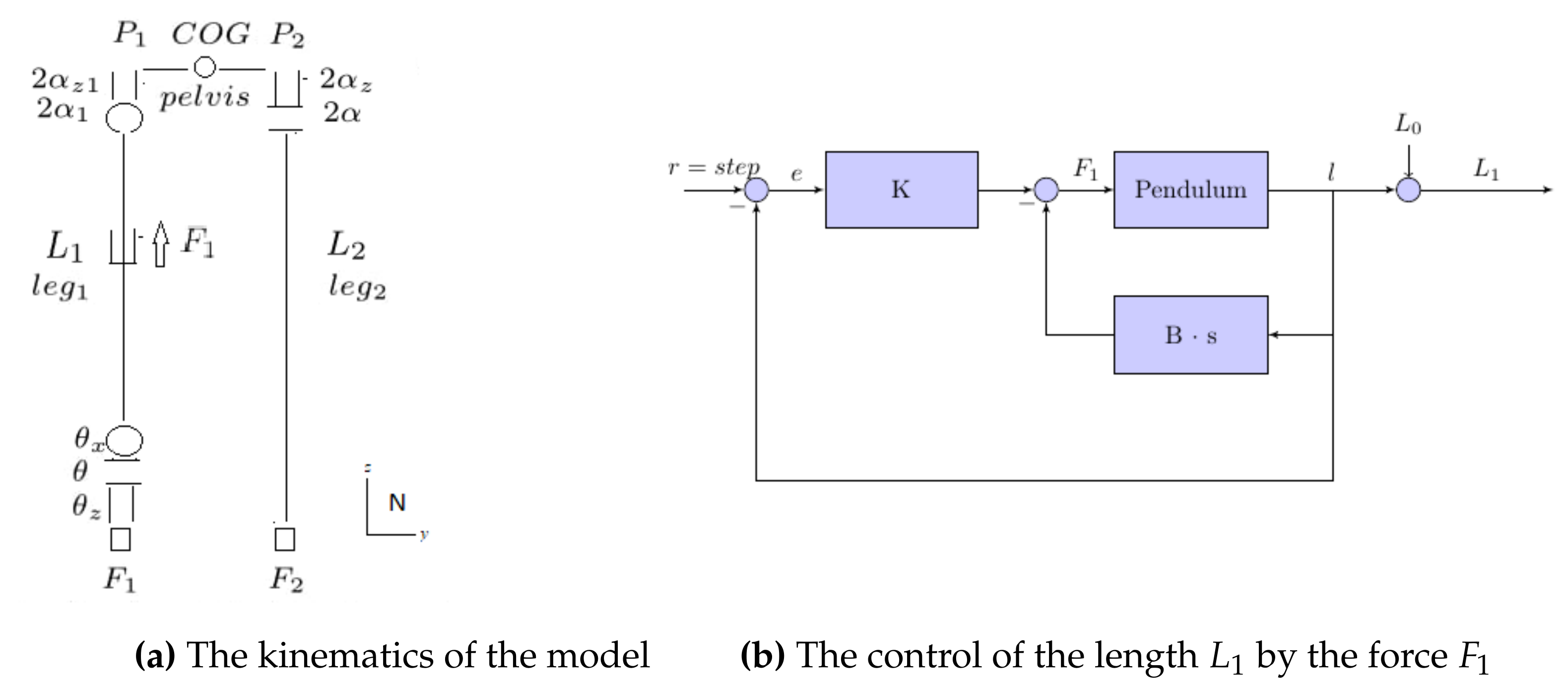
Figure 2.
The COG behaviour.
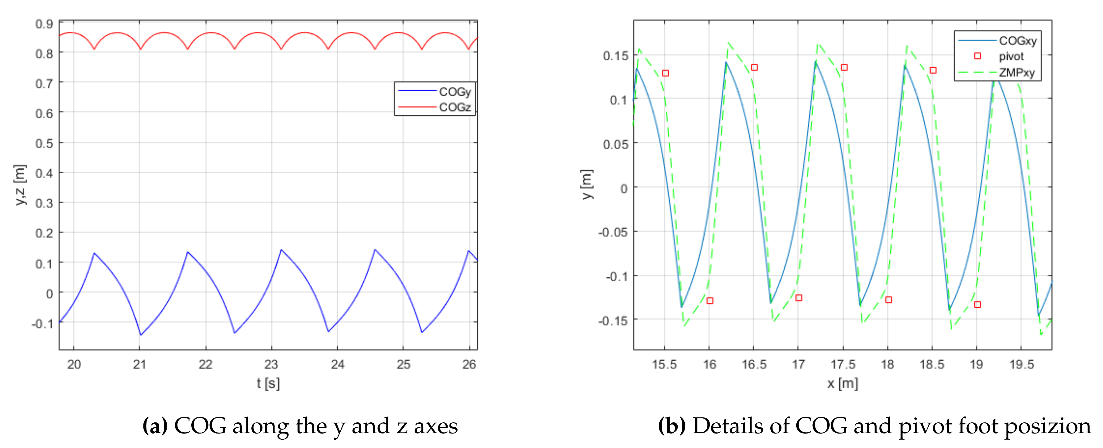
Figure 3.
Angle position and velocity behaviors.
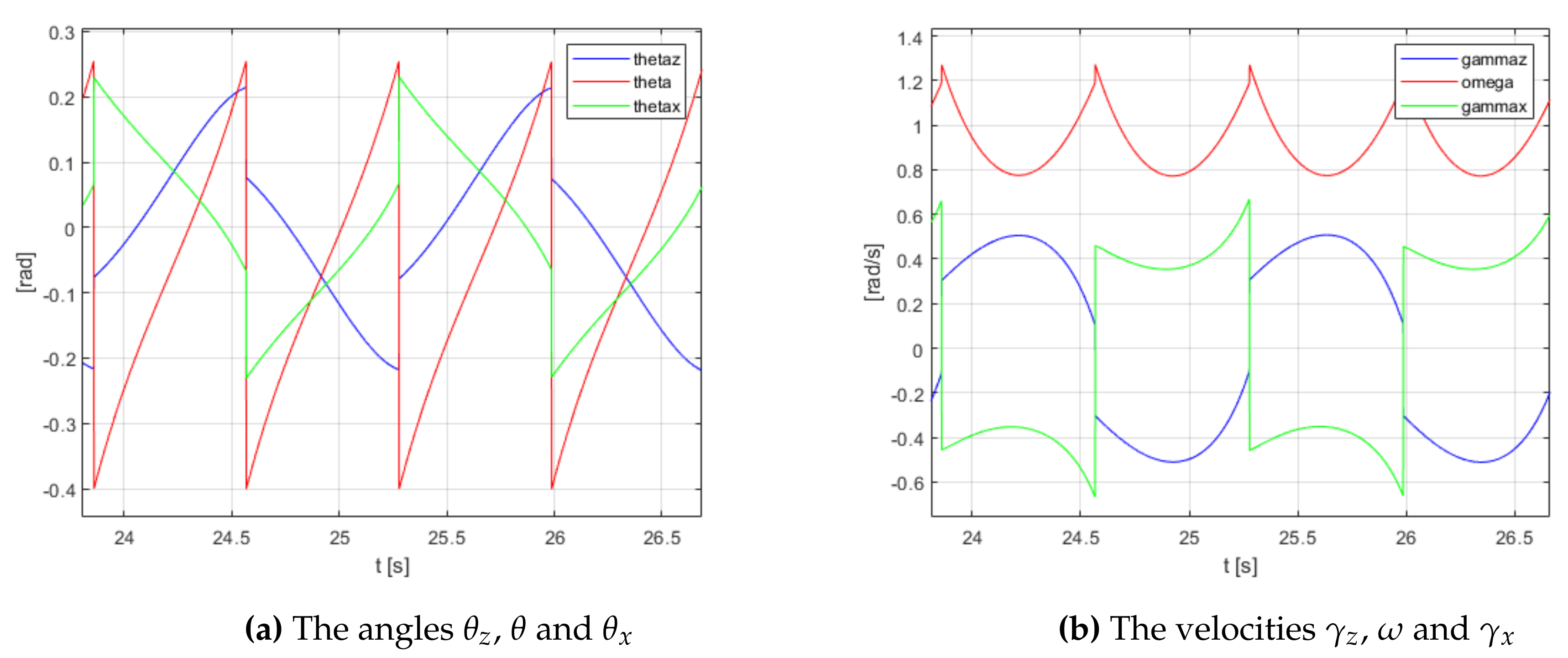
Figure 4.
Total energy and angular momentum ascending a staincase.
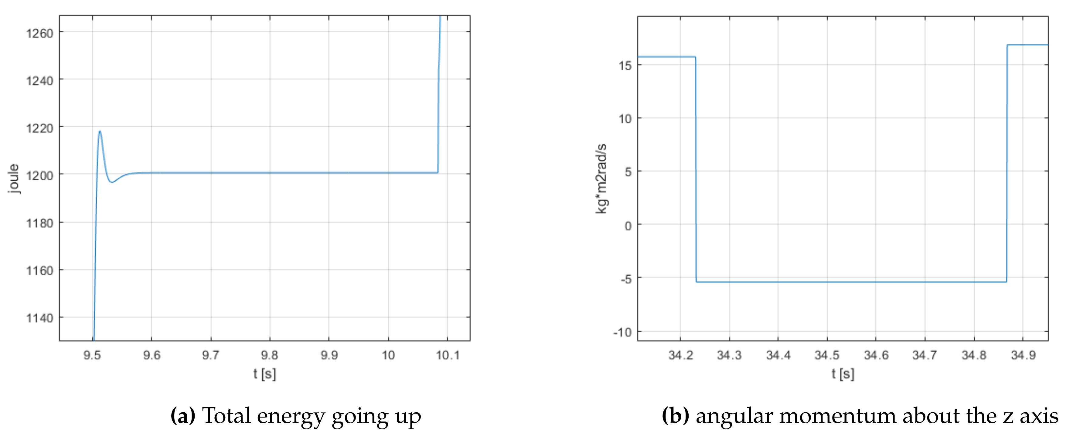
Figure 5.
Length position and velocity of the supporting leg on a staircase with steps of 15 cm.
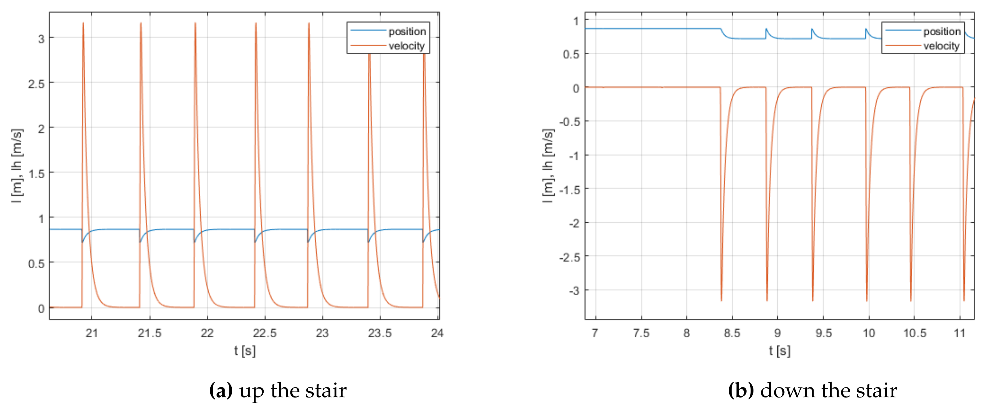
Figure 6.
Different staircases.
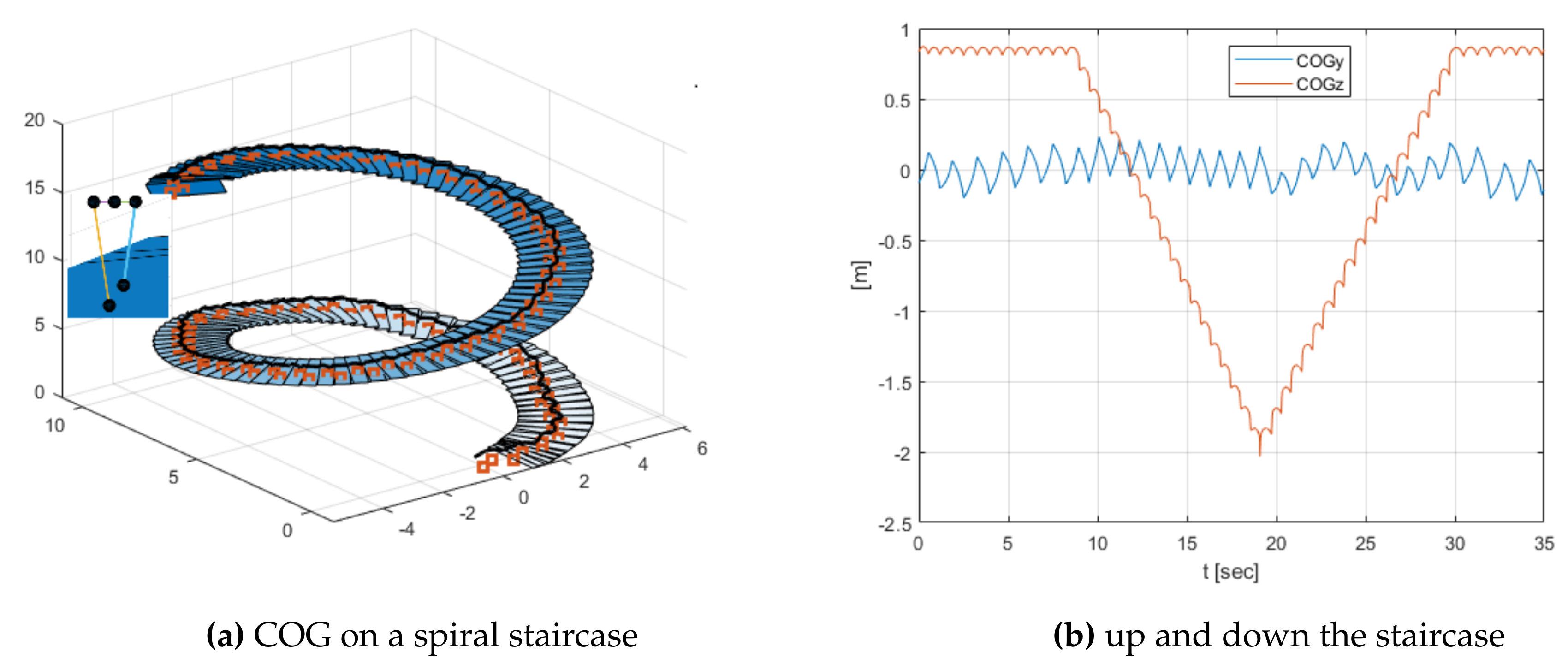
Figure 7.
FPE at the arrival.
Disclaimer/Publisher’s Note: The statements, opinions and data contained in all publications are solely those of the individual author(s) and contributor(s) and not of MDPI and/or the editor(s). MDPI and/or the editor(s) disclaim responsibility for any injury to people or property resulting from any ideas, methods, instructions or products referred to in the content. |
© 2024 by the author. Licensee MDPI, Basel, Switzerland. This article is an open access article distributed under the terms and conditions of the Creative Commons Attribution (CC BY) license (http://creativecommons.org/licenses/by/4.0/).
Copyright: This open access article is published under a Creative Commons CC BY 4.0 license, which permit the free download, distribution, and reuse, provided that the author and preprint are cited in any reuse.


