Submitted:
05 March 2024
Posted:
18 March 2024
You are already at the latest version
Abstract
Keywords:
1. Introduction
2. Background
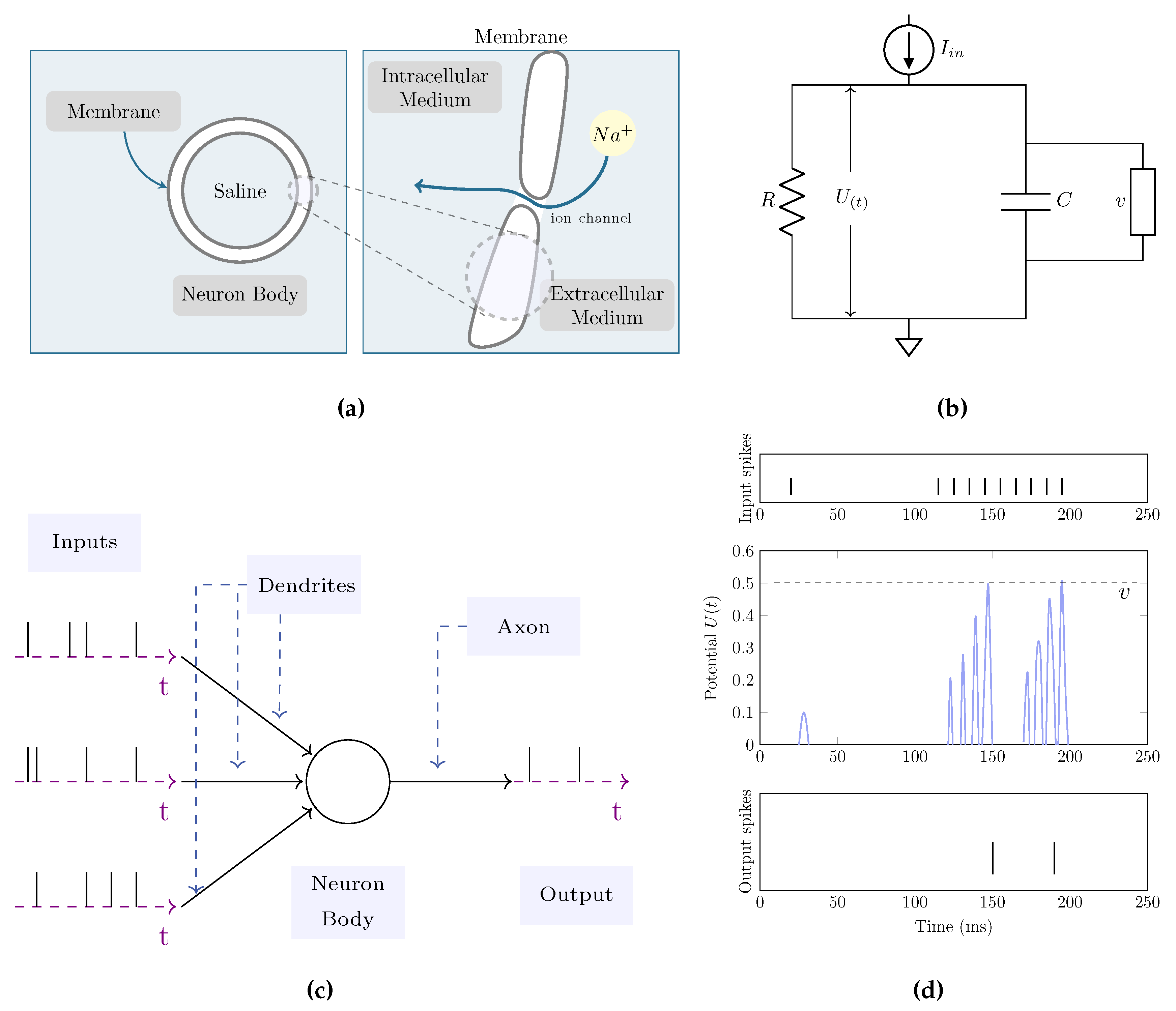
2.1. Spiking Neural Networks
2.2. Long Short-Term Memory
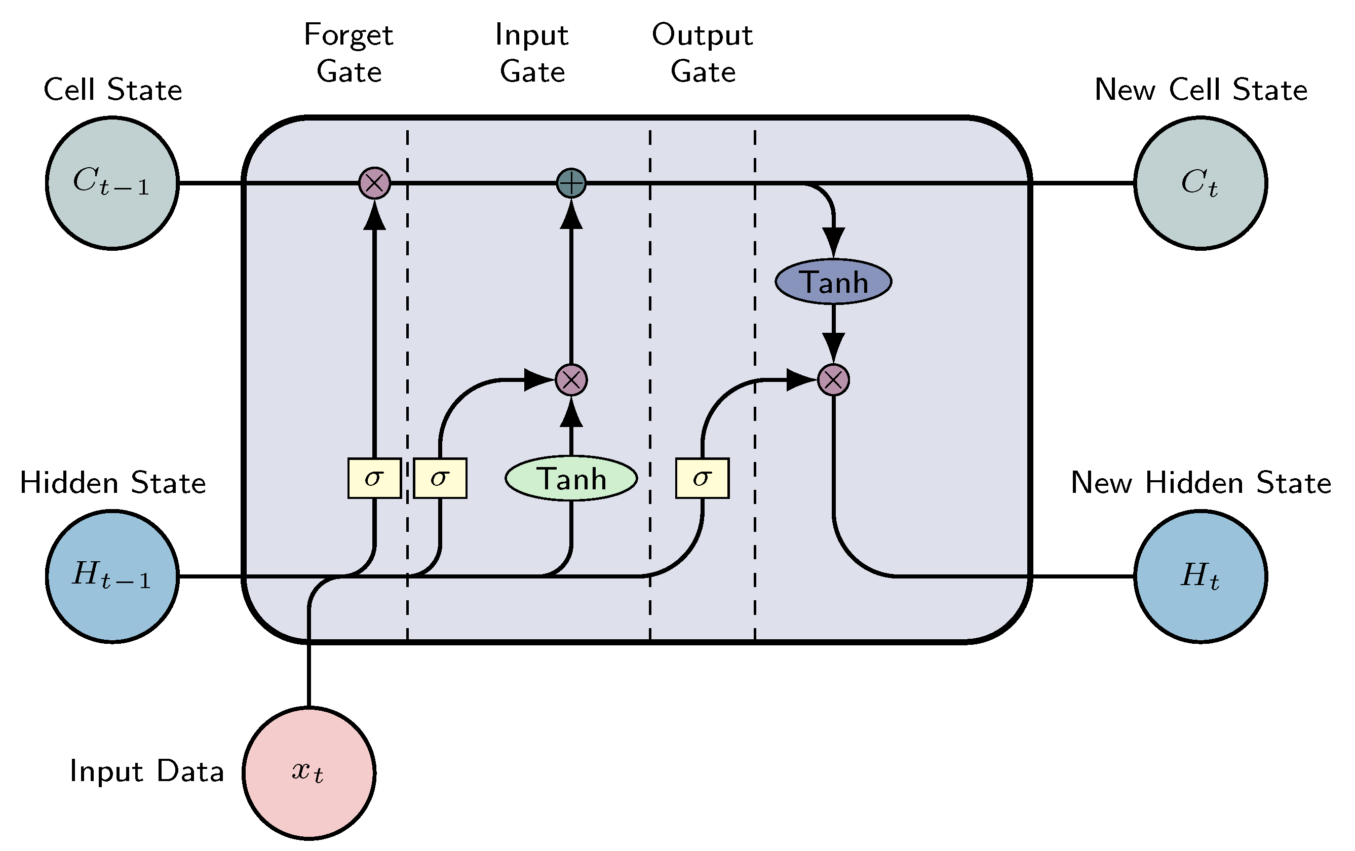
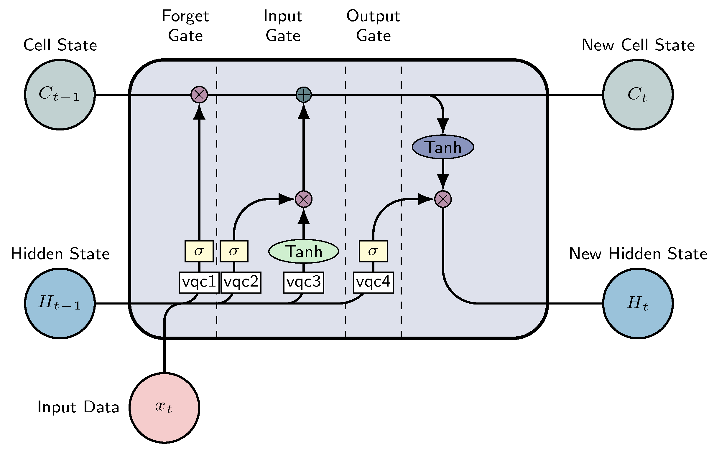
- Cell state: The network’s current long-term memory
- Hidden state: The output from the preceding time step
- The input data in the present time step
-
Forget Gate: This gate decides which information from the cell state is important, considering both the previous hidden state and the new input data. The neural network that implements this gate is build to produce an output closer to 0 when the input data is considered unimportant, and closer to 1 otherwise. To achieve this, we employ the sigmoid activation function. The output values from this gate are then passed upwards and undergo pointwise multiplication with the previous cell state. This pointwise multiplication implies that components of the cell state identified as insignificant by the forget gate network will be multiplied by a value approaching 0, resulting in reduced influence on subsequent steps.To summarize, the forget gate determines which portions of the long-term memory should be disregarded (given less weight) based on the previous hidden state and the new input data.
-
Input gate: Determines the integration of new information into the network’s long-term memory (cell state), considering the prior hidden state and incoming data. The same inputs are utilized, but now with the introduction of a hyperbolic tangent as the activation function. This hyperbolic tangent has learned to blend the previous hidden state with the incoming data, resulting in a newly updated memory vector. Essentially, this vector encapsulates information from the new input data within the context of the previous hidden state. It informs us about the extent to which each component of the network’s long-term memory (cell state) should be updated based on the new information.It should be noted that the utilization of the hyperbolic tangent function in this context is deliberate, owing to its output range confined to [-1,1]. The inclusion of negative values is imperative for this methodology, as it facilitates the attenuation of the impact associated with specific components.
- Output gate: the objective of this gate is to decide the new hidden state by incorporating the newly updated cell state, the prior hidden state, and the new input data. This hidden state has to contain the necessary information while avoiding the inclusion of all learned data. To achieve this, we employ the sigmoid function.
-
The initial step involves determining which information to discard or preserve at the given moment in time. This process is facilitated by the utilisation of the sigmoid function. It examines both the preceding state and the present input , computing the function accordingly:Where and and are weights and biases.
- In this step, the memory cell content undergoes an update by choosing new information for storage within the cell state. The subsequent layer, known as the input gate, comprises two components: the sigmoid function and the hyperbolic tangent (tanh). The sigmoid layer decides which values to update; a value of 1, indicates no change, while a value of 0 results in exclusion. Subsequently, a tanh layer generates a vector of new candidate values, assigning weights to each value based on its significance within the range of -1 to 1. These two components are then combined to update the state:
- The third step consists of updating the previous cell state, with the new cell state, , through two operations: forgetting irrelevant information by scaling the previous state by and incorporating new information from the candidate :
-
Ultimately, the output is calculated through a two-step process. Initially, a sigmoid layer is employed to determine which aspects of the cell state are pertinent for transmission to the output.Subsequently, the cell state undergoes processing via the tanh layer to normalize values between -1 and 1, followed by multiplication with the output of the sigmoid gate.
2.3. Deep Reinforcement Learning
2.4. Quantum Neural Networks
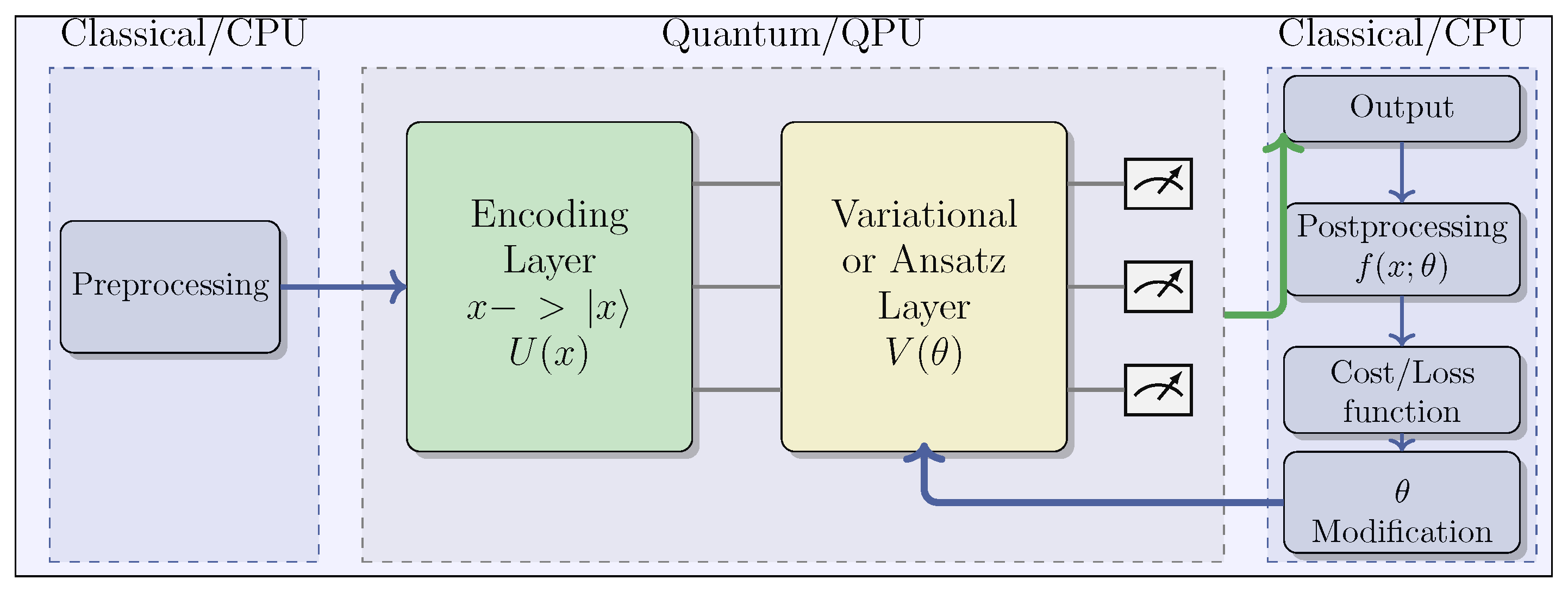
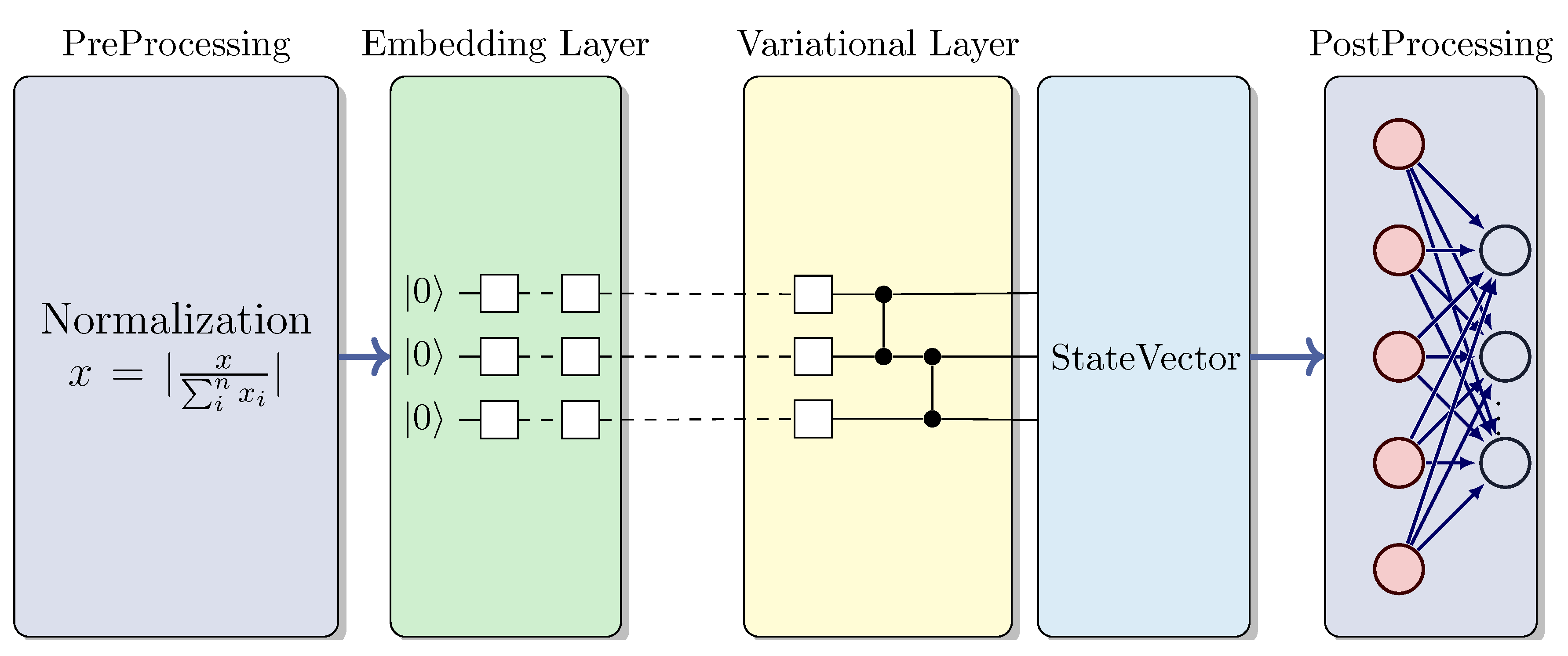
- Pre-processing (CPU): Initial classical data preprocessing, which includes normalization and scaling.
- Quantum Embedding (QPU): Encoding classical data into quantum states through parameterized quantum gates. Various encoding techniques exist, such as angle encoding, also known as tensor product encoding, and amplitude encoding, among others [57].
- Variational Layer (QPU): This layer embodies the functionality of Quantum Neural Networks through the utilization of rotations and entanglement gates with trainable parameters, which are optimized using classical algorithms.
- Measurement Process (QPU/CPU): Measuring the quantum state and decoding it to derive the expected output. The selection of observables employed in this process is critical for achieving optimal performance.
- Post-processing (CPU): Transformation of QPU outputs before feeding them back to the user and integrating them into the cost function during the learning phase.
- Learning (CPU): Computation of the cost function and optimization of ansatz parameters using classic optimization algorithms, such as Adam or SGD. Gradient-free methods, such as SPSA or COLYBA, are also capable of estimating parameter updates.
3. Methodology

4. Experimentation
4.1. Problem Statement
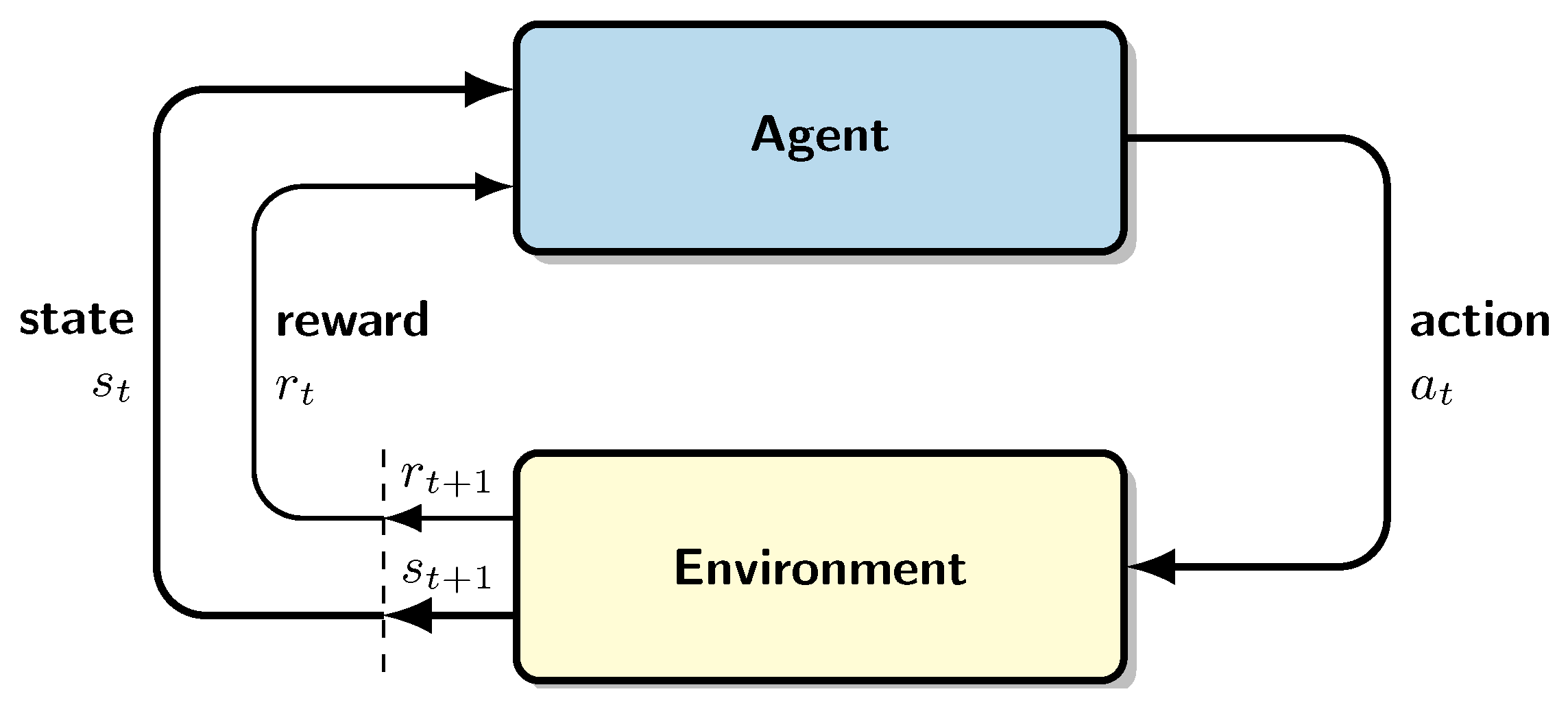
- State space: The state space encompasses 17 attributes; with 14 detailed in Table 1, while the remaining 3 are reserved in case new customized features need to be added.
- Action space: The action space comprises a collection of 10 discrete actions as outlined in Table 2. The temperature bounds for heating and cooling are [12, 23.5] and [21.5, 40] respectively.
-
Reward function: The reward function is formulated as multi-objective, where both energy consumption and thermal discomfort are normalized and added together with different weights. The reward value is consistently non-positive, signifying that optimal behavior yields a cumulative reward of 0. Notice also that there are two temperature comfort ranges defined, one for the summer period and other for the winter period. The weights of each term in the reward allow to adjust the importance of each aspect when environments are evaluated. Finally, the reward function is customizable and can be integrated into the environmentWhere denotes power consumption; is the current indoor temperature; and are the imposed comfort range limits (penalty is 0 if is within this range); represents the weight assigned to power consumption (and consequently, , the comfort weight), and and are scaling constants for consumption and comfort, respectively [67].
4.2. Experimental Settings
4.3. Results
5. Discussion
6. Conclusions and Future Work
7. Patents
Author Contributions
Funding
Institutional Review Board Statement
Informed Consent Statement
Data Availability Statement
Acknowledgments
Conflicts of Interest
Abbreviations
| A2C | Advantage Actor–Critic |
| BPTT | backpropagation through time |
| BG | Basal Ganglia |
| CPU | Central Processing Unit |
| DQN | Deep Q-network |
| DRL | Deep reinforcement learning |
| HDC | Hyperdimensional Computing and Spiking |
| HVAC | Heating, ventilation, air-conditioning |
| KPI | Key performance indicator |
| LIF | Leaky integrate and fired Neuron |
| LSTM | Long/short-term memory |
| LTS | Long-term store |
| mPFC | Medial prefrontal cortex |
| MDP | Markov decision process |
| MLP | Multilayer perceptron |
| NISQ | Noisy, intermediate-scale quantum era |
| PFC | Prefronal Cortex |
| QC | Quantum computing |
| QLIF | Quantum Leaky integrate and fired Neuron |
| QLSTM | Quantum long/short-term memory |
| QML | Quantum machine learning |
| QNN | Quantum neural network |
| QSNN | Quantum spiking neural network |
| QPU | Quantum Processing Unit |
| QRL | Quantum reinforcement learning |
| RNN | Recurrent Neural Networks |
| RL | Reinforcement learning |
| SNN | Spiking neural network |
| S-R | Stimulus-response |
| STS | short-term store |
| vmPFC | Ventromedial prefrontal cortex |
| VQC | Variational quantum circuit |
References
- Zhao, L.; Zhang, L.; Wu, Z.; Chen, Y.; Dai, H.; Yu, X.; Liu, Z.; Zhang, T.; Hu, X.; Jiang, X.; et al. When brain-inspired AI meets AGI. Meta-Radiology 2023, 1, 100005. [CrossRef]
- Fan, C.; Yao, L.; Zhang, J.; Zhen, Z.; Wu, X. Advanced Reinforcement Learning and Its Connections with Brain Neuroscience. Research 2023, 6, 0064, [https://spj.science.org/doi/pdf/10.34133/research.0064]. [CrossRef]
- Domenech, P.; Rheims, S.; Koechlin, E. Neural mechanisms resolving exploitation-exploration dilemmas in the medial prefrontal cortex. Science 2020, 369, eabb0184, [https://www.science.org/doi/pdf/10.1126/science.abb0184]. [CrossRef]
- Baram, A.B.; Muller, T.H.; Nili, H.; Garvert, M.M.; Behrens, T.E.J. Entorhinal and ventromedial prefrontal cortices abstract and generalize the structure of reinforcement learning problems. Neuron 2021, 109, 713–723.e7. [CrossRef]
- Bogacz, R.; Larsen, T. Integration of Reinforcement Learning and Optimal Decision-Making Theories of the Basal Ganglia. Neural computation 2011, 23, 817–51. [CrossRef]
- Houk, J.; Adams, J.; Barto, A. A Model of How the Basal Ganglia Generate and Use Neural Signals that Predict Reinforcement. Models of Information Processing in the Basal Ganglia 1995, Vol. 13.
- Joel, D.; Niv, Y.; Ruppin, E. Actor–critic models of the basal ganglia: new anatomical and computational perspectives. Neural Netw. 2002, 15, 535–547. [CrossRef]
- Collins, A.G.E.; Frank, M.J. Opponent actor learning (OpAL): Modeling interactive effects of striatal dopamine on reinforcement learning and choice incentive. Psychol. Rev. 2014, 121, 337–366. [CrossRef]
- Maia, T.V.; Frank, M.J. From reinforcement learning models to psychiatric and neurological disorders. Nat. Neurosci. 2011, 14, 154–162. [CrossRef]
- Maia, T.V. Reinforcement learning, conditioning, and the brain: Successes and challenges. Cogn. Affect. Behav. Neurosci. 2009, 9, 343–364. [CrossRef]
- O’Doherty, J.; Dayan, P.; Schultz, J.; Deichmann, R.; Friston, K.; Dolan, R.J. Dissociable Roles of Ventral and Dorsal Striatum in Instrumental Conditioning. Science 2004, 304, 452–454, [https://www.science.org/doi/ pdf/10.1126/science.1094285]. [CrossRef]
- Chalmers, E.; Contreras, E.B.; Robertson, B.; Luczak, A.; Gruber, A. Context-switching and adaptation: Brain-inspired mechanisms for handling environmental changes. In Proceedings of the 2016 International Joint Conference on Neural Networks (IJCNN), 2016, pp. 3522–3529. [CrossRef]
- Robertazzi, F.; Vissani, M.; Schillaci, G.; Falotico, E. Brain-inspired meta-reinforcement learning cognitive control in conflictual inhibition decision-making task for artificial agents. Neural Networks 2022, 154, 283–302. [CrossRef]
- Zhao, Z.; Zhao, F.; Zhao, Y.; Zeng, Y.; Sun, Y. A brain-inspired theory of mind spiking neural network improves multi-agent cooperation and competition. Patterns 2023, 4, 100775. [CrossRef]
- Zhang, K.; Lin, X.; Li, M. Graph attention reinforcement learning with flexible matching policies for multi-depot vehicle routing problems. Physica A: Statistical Mechanics and its Applications 2023, 611, 128451. [CrossRef]
- Devlin, J.; Chang, M.W.; Lee, K.; Toutanova, K. BERT: Pre-training of Deep Bidirectional Transformers for Language Understanding, 2019, [arXiv:cs.CL/1810.04805]. [CrossRef]
- Rezayi, S.; Dai, H.; Liu, Z.; Wu, Z.; Hebbar, A.; Burns, A.H.; Zhao, L.; Zhu, D.; Li, Q.; Liu, W.; et al. ClinicalRadioBERT: Knowledge-Infused Few Shot Learning for Clinical Notes Named Entity Recognition. In Proceedings of the Machine Learning in Medical Imaging; Lian, C.; Cao, X.; Rekik, I.; Xu, X.; Cui, Z., Eds., Cham, 2022; pp. 269–278.
- Liu, Z.; He, X.; Liu, L.; Liu, T.; Zhai, X. Context Matters: A Strategy to Pre-train Language Model for Science Education. In Proceedings of the Artificial Intelligence in Education. Posters and Late Breaking Results, Workshops and Tutorials, Industry and Innovation Tracks, Practitioners, Doctoral Consortium and Blue Sky; Wang, N.; Rebolledo-Mendez, G.; Dimitrova, V.; Matsuda, N.; Santos, O.C., Eds., Cham, 2023; pp. 666–674.
- Brown, T.B.; Mann, B.; Ryder, N.; Subbiah, M.; Kaplan, J.; Dhariwal, P.; Neelakantan, A.; Shyam, P.; Sastry, G.; Askell, A.; et al. Language Models are Few-Shot Learners, 2020, [arXiv:cs.CL/2005.14165]. [CrossRef]
- Dosovitskiy, A.; Beyer, L.; Kolesnikov, A.; Weissenborn, D.; Zhai, X.; Unterthiner, T.; Dehghani, M.; Minderer, M.; Heigold, G.; Gelly, S.; et al. An Image is Worth 16x16 Words: Transformers for Image Recognition at Scale, 2021, [arXiv:cs.CV/2010.11929]. [CrossRef]
- Aïmeur, E.; Brassard, G.; Gambs, S. Quantum speed-up for unsupervised learning. Machine Learning 2013, 90, 261–287. [CrossRef]
- Schuld, M.; Bocharov, A.; Svore, K.M.; Wiebe, N. Circuit-centric quantum classifiers. Phys. Rev. A 2020, 101, 032308. [CrossRef]
- Wiebe, N.; Kapoor, A.; Svore, K.M. Quantum Nearest-Neighbor Algorithms for Machine Learning. Quantum Information and Computation 2015, 15, 318–358.
- Anguita, D.; Ridella, S.; Rivieccio, F.; Zunino, R. Quantum optimization for training support vector machines. Neural networks 2003, 16, 763–770. [CrossRef]
- Andrés, E.; Cuéllar, M.P.; Navarro, G. On the Use of Quantum Reinforcement Learning in Energy-Efficiency Scenarios. Energies 2022, 15. [CrossRef]
- Andrés, E.; Cuéllar, M.P.; Navarro, G. Efficient Dimensionality Reduction Strategies for Quantum Reinforcement Learning. IEEE Access 2023, 11, 104534–104553. [CrossRef]
- Busemeyer, J.R.; Bruza, P.D. Quantum Models of Cognition and Decision; Cambridge University Press, 2012.
- Li, J.A.; Dong, D.; Wei, Z.; Liu, Y.; Pan, Y.; Nori, F.; Zhang, X. Quantum reinforcement learning during human decision-making. Nature Human Behaviour 2020, 4, 294–307. [CrossRef]
- Miller, E.K.; Cohen, J.D. An Integrative Theory of Prefrontal Cortex Function. Annual Review of Neuroscience 2001, 24, 167–202. [CrossRef]
- Atkinson, R.; Shiffrin, R. Human Memory: A Proposed System and its Control Processes. In Human Memory: A Proposed System and its Control Processes.; Spence, K.W.; Spence, J.T., Eds.; Academic Press, 1968; Vol. 2, Psychology of Learning and Motivation, pp. 89–195. [CrossRef]
- Andersen, P. The hippocampus book; Oxford university press, 2007.
- Olton, D.S.; Becker, J.T.; Handelmann, G.E. Hippocampus, space, and memory. Behavioral and Brain sciences 1979, 2, 313–322. [CrossRef]
- Raman, N.S.; Devraj, A.M.; Barooah, P.; Meyn, S.P. Reinforcement Learning for Control of Building HVAC Systems. In Proceedings of the 2020 American Control Conference (ACC), 2020, pp. 2326–2332. [CrossRef]
- Wang, Y.; Velswamy, K.; Huang, B. A Long-Short Term Memory Recurrent Neural Network Based Reinforcement Learning Controller for Office Heating Ventilation and Air Conditioning Systems. Processes 2017, 5. [CrossRef]
- Fu, Q.; Han, Z.; Chen, J.; Lu, Y.; Wu, H.; Wang, Y. Applications of reinforcement learning for building energy efficiency control: A review. Journal of Building Engineering 2022, 50, 104165. [CrossRef]
- Hebb, D. The Organization of Behavior: A Neuropsychological Theory; Taylor & Francis, 2005.
- Eshraghian, J.K.; Ward, M.; Neftci, E.; Wang, X.; Lenz, G.; Dwivedi, G.; Bennamoun, M.; Jeong, D.S.; Lu, W.D. Training Spiking Neural Networks Using Lessons From Deep Learning, 2021. [CrossRef]
- Tavanaei, A.; Ghodrati, M.; Kheradpisheh, S.R.; Masquelier, T.; Maida, A. Deep learning in spiking neural networks. Neural Networks 2019, 111, 47–63. [CrossRef]
- Lobo, J.L.; Del Ser, J.; Bifet, A.; Kasabov, N. Spiking Neural Networks and online learning: An overview and perspectives. Neural Networks 2020, 121, 88–100. [CrossRef]
- Lapicque, L. Recherches quantitatives sur l’excitation electrique des nerfs. J. Physiol. Paris. 1907, 9, 620–635.
- Zou, Z.; Alimohamadi, H.; Zakeri, A.; Imani, F.; Kim, Y.; Najafi, M.H.; Imani, M. Memory-inspired spiking hyperdimensional network for robust online learning. Scientific Reports 2022, 12, 7641. [CrossRef]
- Kumarasinghe, K.; Kasabov, N.; Taylor, D. Brain-inspired spiking neural networks for decoding and understanding muscle activity and kinematics from electroencephalography signals during hand movements. Scientific Reports 2021, 11, 2486. [CrossRef]
- Banino, A.; Barry, C.; Uria, B.; Blundell, C.; Lillicrap, T.; Mirowski, P.; Pritzel, A.; Chadwick, M.J.; Degris, T.; Modayil, J.; et al. Vector-based navigation using grid-like representations in artificial agents. Nature 2018, 557, 429–433. [CrossRef]
- Bengio, Y.; Simard, P.; Frasconi, P. Learning long-term dependencies with gradient descent is difficult. IEEE Transactions on Neural Networks 1994, 5, 157–166. [CrossRef]
- Graves, A.; Liwicki, M.; Fernández, S.; Bertolami, R.; Bunke, H.; Schmidhuber, J. A Novel Connectionist System for Unconstrained Handwriting Recognition. IEEE Transactions on Pattern Analysis and Machine Intelligence 2009, 31, 855–868. [CrossRef]
- Graves, A.; Schmidhuber, J. Framewise phoneme classification with bidirectional LSTM and other neural network architectures. Neural networks: the official journal of the International Neural Network Society 2005, 18, 602–610. [CrossRef]
- Hochreiter, S.; Schmidhuber, J. LSTM can solve hard long time lag problems. Advances in Neural Information Processing Systems 1996, 9, 473–479.
- Triche, A.; Maida, A.S.; Kumar, A. Exploration in neo-Hebbian reinforcement learning: Computational approaches to the exploration–exploitation balance with bio-inspired neural networks. Neural Networks 2022, 151, 16–33. [CrossRef]
- Dong, H.; Ding, Z.; Zhang, S.; Yuan, H.; Zhang, H.; Zhang, J.; Huang, Y.; Yu, T.; Zhang, H.; Huang, R. Deep Reinforcement Learning: Fundamentals, Research, and Applications; Springer Nature, 2020. http://www.deepreinforcementlearningbook.org.
- Sutton, R.S.; Barto, A.G., The Reinforcement Learning Problem. In Reinforcement Learning: An Introduction; MIT Press, 1998; pp. 51–85.
- Mnih, V.; Kavukcuoglu, K.; Silver, D.; Rusu, A.A.; Veness, J.; Bellemare, M.G.; Graves, A.; Riedmiller, M.; Fidjeland, A.K.; Ostrovski, G.; et al. Human-level control through deep reinforcement learning. Nature 2015, 518, 529–533. [CrossRef]
- Shao, K.; Zhao, D.; Zhu, Y.; Zhang, Q. Visual Navigation with Actor-Critic Deep Reinforcement Learning. In Proceedings of the 2018 International Joint Conference on Neural Networks (IJCNN), 2018, pp. 1–6. [CrossRef]
- Macaluso, A.; Clissa, L.; Lodi, S.; Sartori, C. A Variational Algorithm for Quantum Neural Networks. In Proceedings of the Computational Science – ICCS 2020. Springer International Publishing, 2020, pp. 591–604.
- Benedetti, M.; Lloyd, E.; Sack, S.; Fiorentini, M. Parameterized quantum circuits as machine learning models. Quantum Science and Technology 2019, 4, 043001. [CrossRef]
- Zhao, C.; Gao, X.S. QDNN: deep neural networks with quantum layers. Quantum Machine Intelligence 2021, 3, 15. [CrossRef]
- Wittek, P. Quantum Machine Learning: What Quantum Computing means to data mining; Elsevier, 2014.
- Weigold, M.; Barzen, J.; Leymann, F.; Salm, M. Expanding Data Encoding Patterns For Quantum Algorithms. In Proceedings of the 2021 IEEE 18th International Conference on Software Architecture Companion (ICSA-C), 2021, pp. 95–101. [CrossRef]
- McCloskey, M.; Cohen, N.J. Catastrophic Interference in Connectionist Networks: The Sequential Learning Problem. In Catastrophic Interference in Connectionist Networks: The Sequential Learning Problem; Bower, G.H., Ed.; Academic Press, 1989; Vol. 24, Psychology of Learning and Motivation, pp. 109–165. [CrossRef]
- Zenke, F.; Poole, B.; Ganguli, S. Continual Learning Through Synaptic Intelligence. In Proceedings of the Proceedings of the 34th International Conference on Machine Learning; Precup, D.; Teh, Y.W., Eds. PMLR, 06–11 Aug 2017, Vol. 70, Proceedings of Machine Learning Research, pp. 3987–3995.
- Rusu, A.A.; Rabinowitz, N.C.; Desjardins, G.; Soyer, H.; Kirkpatrick, J.; Kavukcuoglu, K.; Pascanu, R.; Hadsell, R. Progressive Neural Networks. CoRR 2016, abs/1606.04671, [1606.04671]. [CrossRef]
- Shin, H.; Lee, J.K.; Kim, J.; Kim, J. Continual Learning with Deep Generative Replay. CoRR 2017, abs/1705.08690, [1705.08690]. [CrossRef]
- Kirkpatrick, J.; Pascanu, R.; Rabinowitz, N.C.; Veness, J.; Desjardins, G.; Rusu, A.A.; Milan, K.; Quan, J.; Ramalho, T.; Grabska-Barwinska, A.; et al. Overcoming catastrophic forgetting in neural networks. CoRR 2016, abs/1612.00796, [1612.00796]. [CrossRef]
- Eshraghian, J.K.; Ward, M.; Neftci, E.; Wang, X.; Lenz, G.; Dwivedi, G.; Bennamoun, M.; Jeong, D.S.; Lu, W.D. Training spiking neural networks using lessons from deep learning. Proceedings of the IEEE 2023, 111, 1016–1054. [CrossRef]
- Crawley, D.; Pedersen, C.; Lawrie, L.; Winkelmann, F. EnergyPlus: Energy Simulation Program. Ashrae Journal 2000, 42, 49–56.
- Mattsson, S.E.; Elmqvist, H. Modelica - An International Effort to Design the Next Generation Modeling Language. IFAC Proceedings Volumes 1997, 30, 151–155. 7th IFAC Symposium on Computer Aided Control Systems Design (CACSD ’97), Gent, Belgium, 28-30 April. [CrossRef]
- Zhang, Z.; Lam, K.P. Practical Implementation and Evaluation of Deep Reinforcement Learning Control for a Radiant Heating System. In Proceedings of the Proceedings of the 5th Conference on Systems for Built Environments, New York, NY, USA, 2018; BuildSys ’18, p. 148–157. [CrossRef]
- Jiménez-Raboso, J.; Campoy-Nieves, A.; Manjavacas-Lucas, A.; Gómez-Romero, J.; Molina-Solana, M. Sinergym: A Building Simulation and Control Framework for Training Reinforcement Learning Agents. In Proceedings of the Proceedings of the 8th ACM International Conference on Systems for Energy-Efficient Buildings, Cities, and Transportation, New York, NY, USA, 2021; p. 319–323. [CrossRef]
- Scharnhorst, P.; Schubnel, B.; Fernández Bandera, C.; Salom, J.; Taddeo, P.; Boegli, M.; Gorecki, T.; Stauffer, Y.; Peppas, A.; Politi, C. Energym: A Building Model Library for Controller Benchmarking. Applied Sciences 2021, 11. [CrossRef]
- Triche, A.; Maida, A.S.; Kumar, A. Exploration in neo-Hebbian reinforcement learning: Computational approaches to the exploration–exploitation balance with bio-inspired neural networks. Neural Networks 2022, 151, 16–33. [CrossRef]
- Hill, F.; Lampinen, A.; Schneider, R.; Clark, S.; Botvinick, M.; McClelland, J.L.; Santoro, A. Environmental drivers of systematicity and generalization in a situated agent, 2020, [arXiv:cs.AI/1910.00571]. [CrossRef]
- Lake, B.M.; Baroni, M. Generalization without systematicity: On the compositional skills of sequence-to-sequence recurrent networks, 2018, [arXiv:cs.CL/1711.00350]. [CrossRef]
- Botvinick, M.; Wang, J.X.; Dabney, W.; Miller, K.J.; Kurth-Nelson, Z. Deep Reinforcement Learning and Its Neuroscientific Implications. Neuron 2020, 107, 603–616. [CrossRef]

| Name | Units |
|---|---|
| Site-Outdoor-Air-DryBulb-Temperature | °C |
| Site-Outdoor-Air-Relative-Humidity | % |
| Site-Wind-Speed | m/s |
| Site-Wind-Direction | degree from north |
| Site-Diffuse-Solar-Radiation-Rate-per-Area | W/m2 |
| Site-Direct-Solar-Radiation-Rate-per-Area | W/m2 |
| Zone-Thermostat-Heating-Setpoint-Temperature | °C |
| Zone-Thermostat-Cooling-Setpoint-Temperature | °C |
| Zone-Air-Temperature | °C |
| Zone-Air-Relative-Humidity | % |
| Zone-People-Occupant-Count | count |
| Environmental-Impact-Total-CO2-Emissions-Carbon-Equivalent-Mass | Kg |
| Facility-Total-HVAC-Electricity-Demand-Rate | W |
| Total-Electricity-HVAC | W |
| Name | Heating Target Temperature | Cooling Target Temperature |
|---|---|---|
| 0 | 13 | 37 |
| 1 | 14 | 34 |
| 2 | 15 | 32 |
| 3 | 16 | 30 |
| 4 | 17 | 30 |
| 5 | 18 | 30 |
| 6 | 19 | 27 |
| 7 | 20 | 26 |
| 8 | 21 | 25 |
| 9 | 21 | 24 |
| MLP | SNN | LSTM | |
|---|---|---|---|
| Optimizer | Adam(lr=1e-4) | Adam(lr=1e-3) | Adam(lr=1e-3) |
| Batch Size | 32 | 16 | 32 |
| BetaEntropy | 0.01 | 0.01 | 0.01 |
| Discount Factor | 0.98 | 0.98 | 0.98 |
| Steps | - | 15 | - |
| Hidden | - | 15 | 25 |
| Layers | Actor: [Linear[17, 450], ReLU | Actor: [Linear[17, 15] | Actor:[LSTM(17, 25, layers=5) |
| Linear[450, 10]] | Lif1, Lif2 | Linear[25, 10]] | |
| Linear[15, 10]] | |||
| Critic: [Linear[17, 450], ReLU | Critic: [Linear[17, 15] | ||
| Linear[450, 1]] | Lif1, Lif2 | Critic: [LSTM(17, 25, layers=5) | |
| Linear[15, 1]] | Linear[25, 1]] |
| QNN | QSNN | QLSTM | QSNN-QLSTM | |
|---|---|---|---|---|
| Optimizer | Adam(lr=1e-2) | Adam(lr=1e-3) | Adam(lr=1e-3) | [(Adam(QSNN.parameters,lr= 1e-2), |
| Adam(QLSTM.parameters, lr=1e-2))] | ||||
| Batch Size | 128 | 16 | 128 | 128 |
| Pre-processing | Normalization | Normalization | - | Normalization |
| Post-processing | - | - | - | - |
| BetaEntropy | 0.01 | 0.01 | 0.01 | 0.01 |
| Discount Factor | 0.98 | 0.98 | 0.98 | 0.98 |
| Steps | - | 15 | 15 | 15 |
| Hidden | - | 15 | 25 | 15 (QSNN), 125 (QLSTM) |
| Layers | Actor: [[5 QNN] | Actor: [ Linear[17, 15] | Actor: [ Linear[17, 42] | |
| ReLU | 15 QSNN | Linear[42, 5] | ||
| Linear[, 10]] | Linear[15, 10]] | 4 VQCs | ||
| Linear[25, 5] | ||||
| Linear[5, 25] | ||||
| Linear[25, 10]] | ||||
| Critic: [[5 QNN | Critic: [ Linear[17, 15] | Critic: [ Linear[17, 42] | 5 QSNN | |
| ReLU | 15 QSNN | Linear[42, 5] | 5 QLSTM | |
| Linear[, 1]] | Linear[15, 1]] | 4 VQC´S | ||
| Linear[25, 5] | ||||
| Linear[5, 25] | ||||
| Linear[25, 1]] | ||||
| Qubits | 5 | 5 | 5 | 5 |
| Encoding Strategy | Amplitud Encoding | Amplitud Encoding | Angle Encoding | Amplitud Encoding |
| Average Tot.Reward | Best Tot.Reward | Worst Tot.Reward | Test Reward | Time (s) | |
|---|---|---|---|---|---|
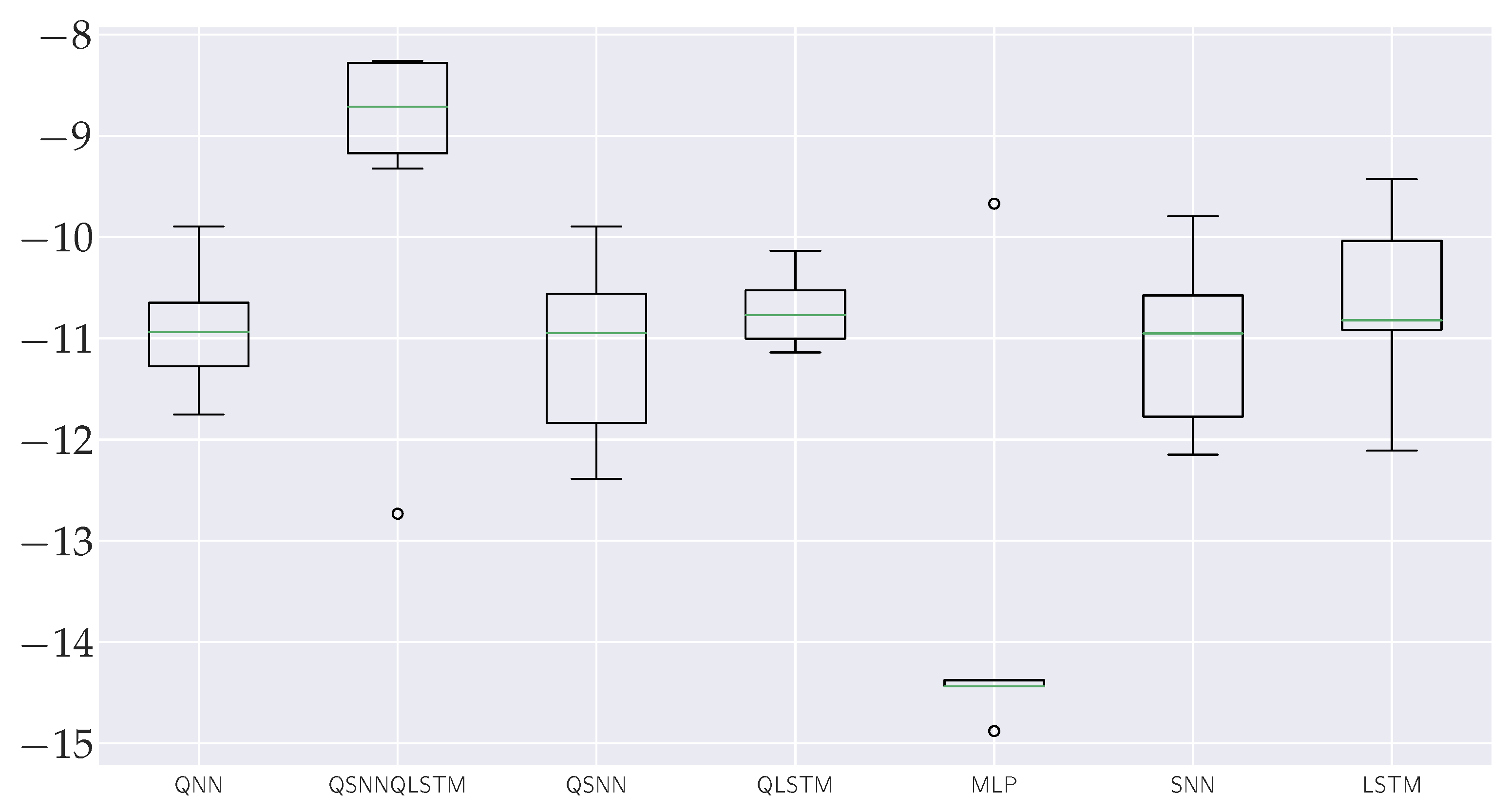
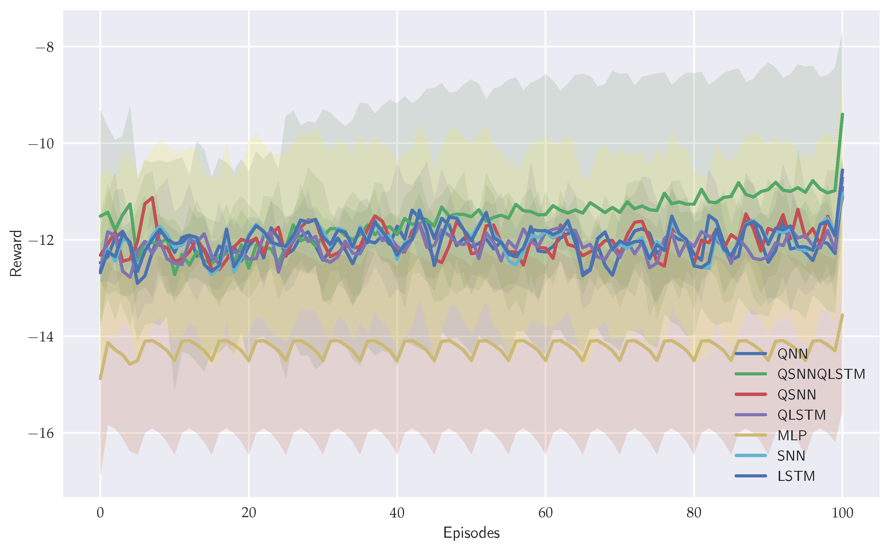
| MLP | -13.75 | -9.67 | -14.88 | -13.25 | 297.8 |
| SNN | -11.05 | -9.79 | -12.15 | -13.31 | 307.6 |
| LSTM | -10.56 | -9.43 | -12.11 | -12.67 | 302.8 |
| QNN | -10.92 | -9.90 | -11.75 | -12.87 | 326.1 |
| QSNN | -11.12 | -9.89 | -12.39 | -13.32 | 467.4 |
| QLSTM | -10.72 | -10.14 | -11.14 | -12.19 | 335.42 |
| QSNN-QLSTM | -9.40 | -8.26 | -12.73 | -11.83 | 962.5 |
Disclaimer/Publisher’s Note: The statements, opinions and data contained in all publications are solely those of the individual author(s) and contributor(s) and not of MDPI and/or the editor(s). MDPI and/or the editor(s) disclaim responsibility for any injury to people or property resulting from any ideas, methods, instructions or products referred to in the content. |
© 2024 by the authors. Licensee MDPI, Basel, Switzerland. This article is an open access article distributed under the terms and conditions of the Creative Commons Attribution (CC BY) license (http://creativecommons.org/licenses/by/4.0/).


