1. Introduction and Background
Airfoils designed for low Reynolds numbers play crucial roles in various applications, including Mini Unmanned Aerial Vehicles (UAVs), which are instrumental in executing high-definition remote sensing, infrastructure surveillance, 3D mapping, and photogrammetry tasks [
1,
2,
3]. Additionally, they are vital for Small-Scale Wind Turbines (SSWTs), contributing to the reduction of electrical grid demands and greenhouse gas emissions [
4]. To maximize the performance of these technologies, the airfoils must be specifically designed to meet their unique requirements. Techniques for optimizing airfoil design frequently include the use of genetic algorithms, surrogate-based modeling, and artificial neural networks [
5,
6].
This study enhances the development of machine/deep learning approaches for airfoil optimization by generating a dataset with lift, drag, and parameterization coefficients for 2900 airfoils at a Reynolds number of
. The lift and drag coefficients were generated using the CFD approach implemented in OpenFOAM [
7]. It employs the Class Shape Transformation (CST) method [
8] to describe the curve of each airfoil. Additionally, the CST method was applied to augment the point count in each airfoil’s ’.dat’ file, improving the accuracy of the mesh. The dataset also incorporates these refined coordinates from every ‘.dat’ file.
2. Methodology
2.1. Airfoil Profile
The initial airfoil ’.dat’ files were obtained from the UIUC Airfoil Data Site [
9] and the Airfoil Tools [
10] online databases. The ’.dat’ files were downloaded from the UIUC Airfoil Data Site using a Python script developed by Josh [
11], and those from the Airfoil Tools site were downloaded manually. The ’.dat’ files thus obtained were of varying number of points, and hence, this was a major consideration during the automation of the Class Shape Transformation (CST) process. The study exclusively utilized ’.dat’ files in the Selig format. In this format, the coordinate system begins at (1, 0), advances to the leading edge, and then returns to (1, 0) via the lower surface.
2.2. Class Shape Transformation (CST) Parametrization Technique
CST (Class-Shape Transformation) or Kulfan airfoils constitute a group of airfoil profiles characterized by a parameterized representation of their upper and lower surfaces. The CST approach is a versatile parameterization strategy for crafting both two-dimensional and three-dimensional forms. Utilizing a class function alongside a shape function, the CST method encapsulates an airfoil’s form, ensuring a closed trailing edge. Introduced by Kulfan [
8], this parameterization technique delineates a two-dimensional figure through the integration of a class function C(
) and a shape function S(
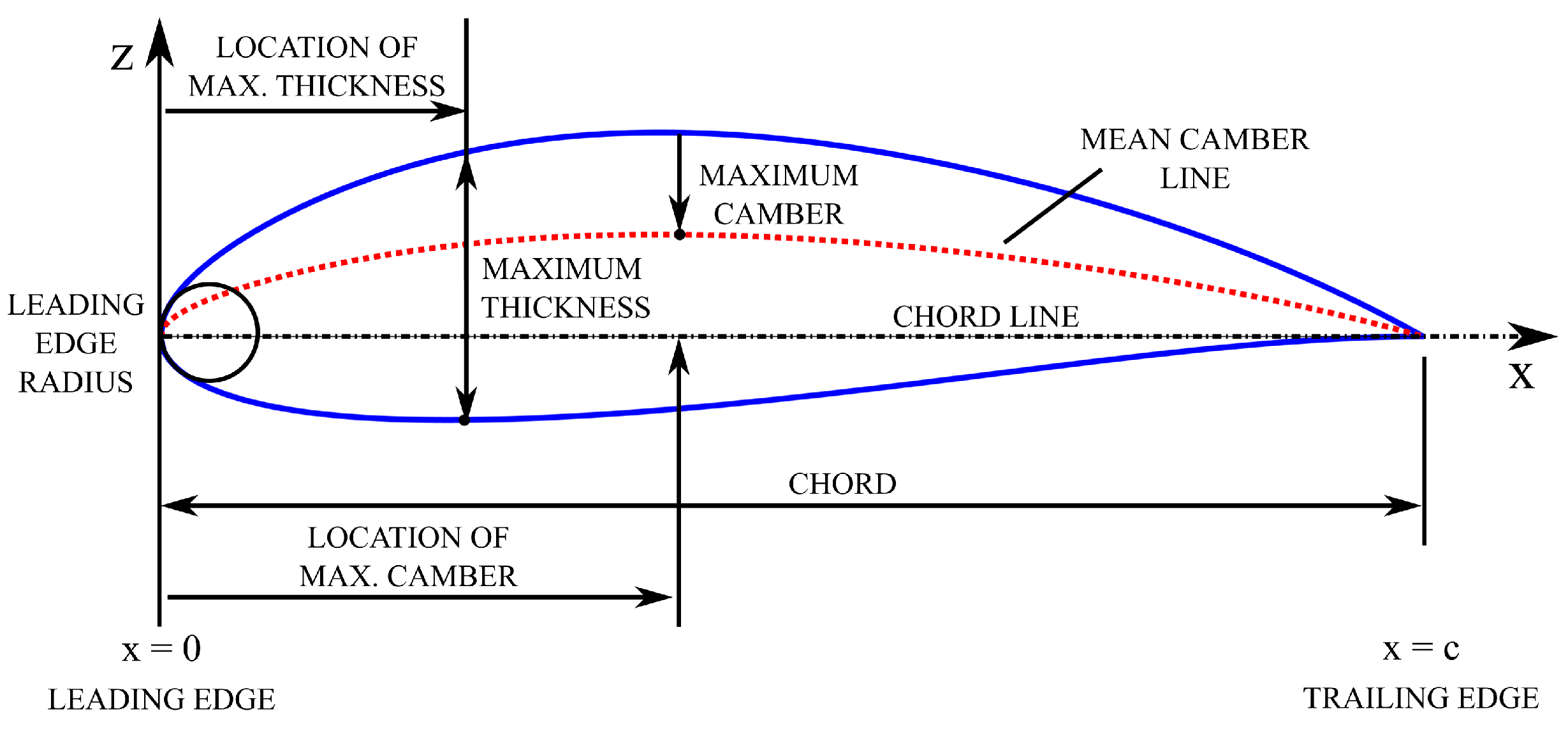
), augmented by a component that delineates the trailing edge’s thickness. The construction of an airfoil via the CST method involves aggregating the contributions from its foundational function, crafted using Bernstein polynomials. For initial airfoil design and optimization, CST employing lower-order polynomials is preferred due to its minimal parameter requirement for defining specific airfoil shapes. Although intricate, CST can be adapted to a wide array of aerodynamic body shapes without necessitating a predefined geometry. This methodology offers precise control over critical features such as the leading-edge radius, boat-tail angle, and trailing edge thickness, making it applicable in both aerodynamic studies and optimization endeavors.
2.2.1. CST Formulation
The general form of the mathematical expression that represents a typical airfoil geometry is:
where
,
and
. The term
corresponds to the round nose of the airfoil. Similarly, the term
corresponds to the sharp trailing edge of the airfoil. The term
controls the thickness of the trailing edge, and the summation term is a general function that describes the shape of the airfoil between the round nose and the sharp trailing edge.
The CST parameters are given as follows (Adapted from [
12]),
2.2.2. Airfoil Shape and Class Function
The shape function
is given by the relation,
The term
defines the class function
given by,
Typically, the parameters N1 and N2 are set to 0.5 and 1 for an airfoil with a rounded nose. The class function delineates broad categories of geometric forms, while the shape function specifies the exact contours within a particular geometric category.
Defining an airfoil shape function and specifying its geometry class is equivalent to defining the actual airfoil coordinates, which can then be obtained from the combination of the shape and class functions from the relation,
The airfoil is then defined using the Bernstein polynomials, which are defined for the order n as follows,
The binomial coefficients are defined as,
The first term of the polynomial defines the leading-edge radius, and the last term is the boat-tail angle. The terms that fall in between serve as the "shaping terms". Here, a Bernstein polynomial of the eighth order is employed, resulting in eight weighted coefficients upon completion of the CST process. The upper surface of the airfoil is defined by the equations,
The lower surface of the airfoil is defined by the equations,
where,
The selection of an eighth order Bernstein polynomial was justified by its drag predictions and pressure distribution which perfectly matched experimental observations.
2.2.3. Key Observations
Throughout the process of airfoil parameterization, several key findings emerged that deserve attention. Notably, when the leading edge point deviated from the origin (0,0) with a y-offset, the airfoils generated through the CST method exhibited a marked increase in error percentage. This deviation significantly altered the airfoil’s curvature, rendering it beyond the capture capability of the ’blockMesh’ utility. Additionally, a significant portion of the airfoils had their trailing edges positioned away from (1,0), challenging the meshing process, which necessitates a trailing edge at (1,0). Consequently, airfoils not meeting this criterion were excluded from the preliminary airfoil database. The comparison between the original and the derived airfoils showed only a minimal error margin. This approach was developed utilizing MATLAB
® building on the work of Pramudita Satria Palar [
13].
2.2.4. Shape Generation
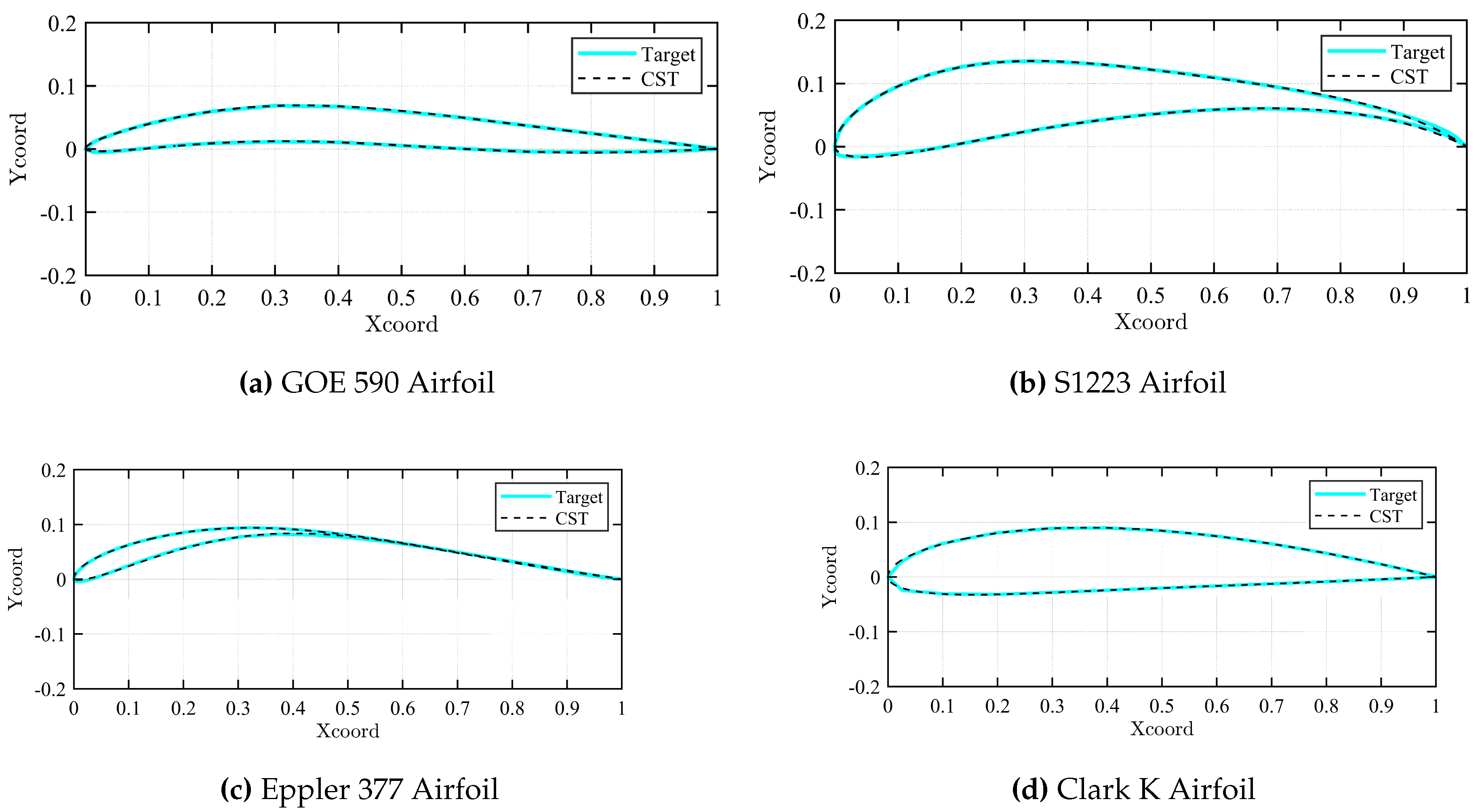
Figure 2 illustrates several different airfoil sections created through the CST framework.
2.3. Geometry
The CST framework was used to create airfoils that were 1 meter in length. Enhancing the ".dat" file with more points leads to more precise simulations by better representing the airfoil’s shape. The CST code generates the ".dat" file containing a specified number of points distributed evenly. Simulations were conducted using airfoils defined by 100, 300, 600, 1000 and 2000 points. The findings indicated that the number of points beyond 600 did not affect the simulation outcomes. Therefore, ".dat" files with 600 points were established as the standard for subsequent simulations.
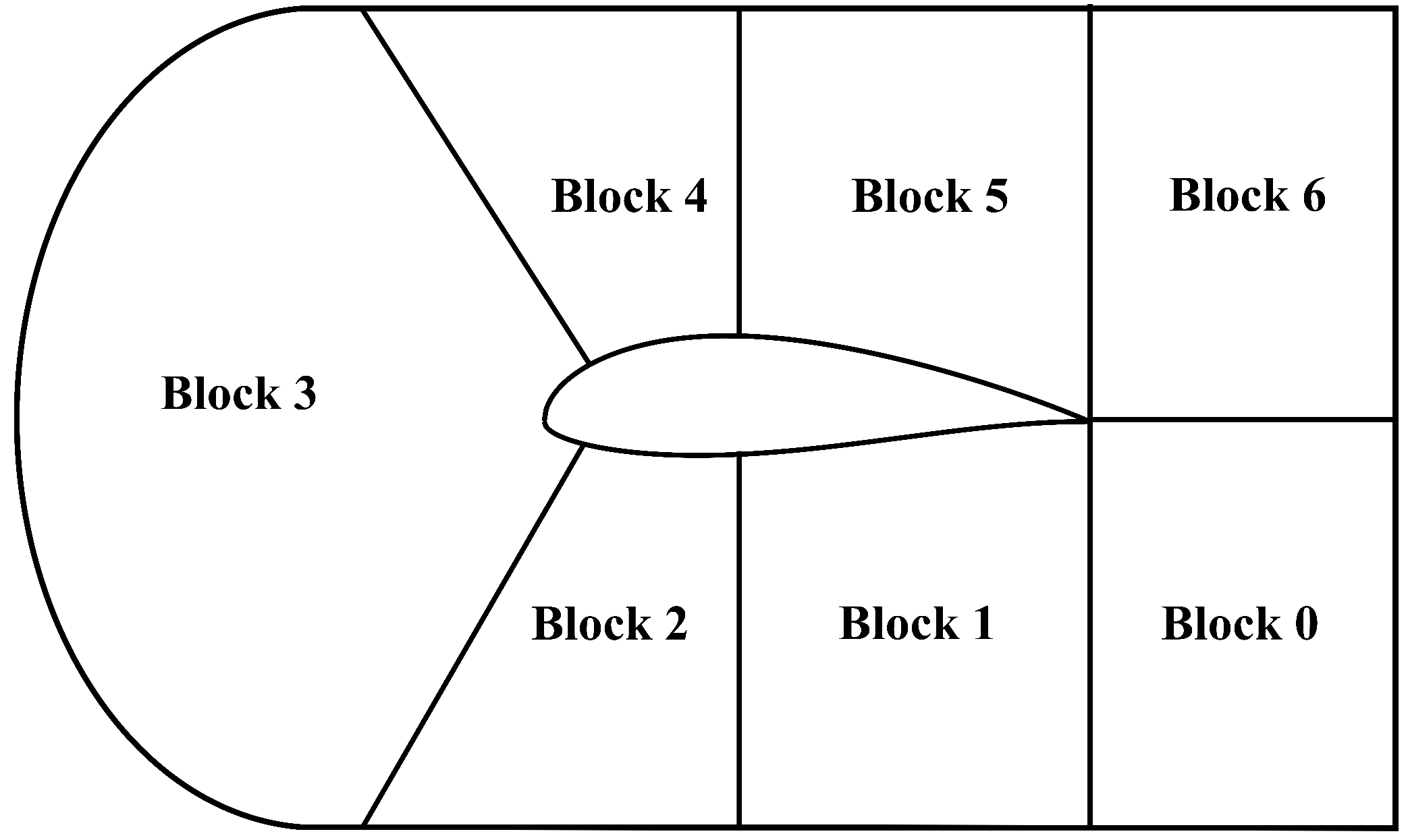
The computational domain was designed with a C-type layout, maintaining an 11 chord length distance on average from the far field. The curved surface and both the top and bottom surfaces were assigned the role of flow inlet boundary, whereas the outlet condition was applied to the right-side wall. The domain is divided into seven blocks as shown in
Figure 3, with blocks 0, 1, and 2 serving as reflections of blocks 6, 5, and 4, respectively, across the chord line of the airfoil. The airfoil coordinates were interconnected using the OpenFOAM ’PolyLine’ segments. However, as the ’Polyline’ edges were not effectively capturing the airfoil’s leading edge curvature, an additional block (block 3) was formed where the airfoil coordinates were connected through the OpenFOAM ’Spline’ curve segments.
2.4. Mesh Setup and Details
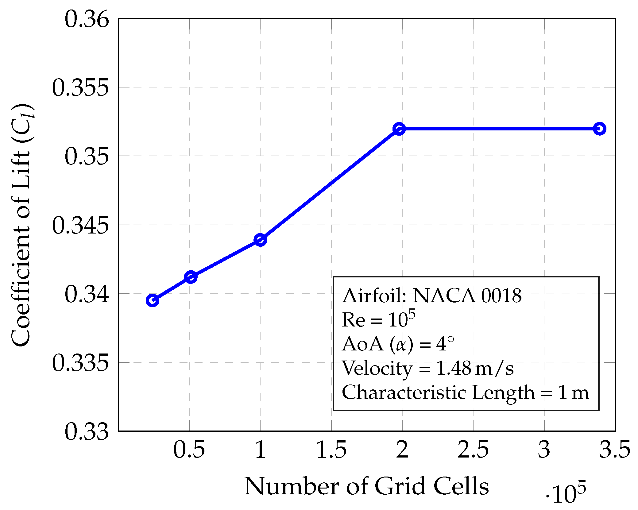
This study utilized the OpenFOAM ’blockMesh’ mesh generation utility. Initially, a study on mesh independence was conducted to assess the impact of the quantity and dimensions of mesh cells on the outcome of the simulation. It was observed that an increase in the number of cells typically enhances the accuracy of the simulation, albeit at the cost of increased computational time and resources. This study of grid independence involved a comparison of the lift coefficient for the symmetric NACA 0018 airfoil at a 4° angle of attack.
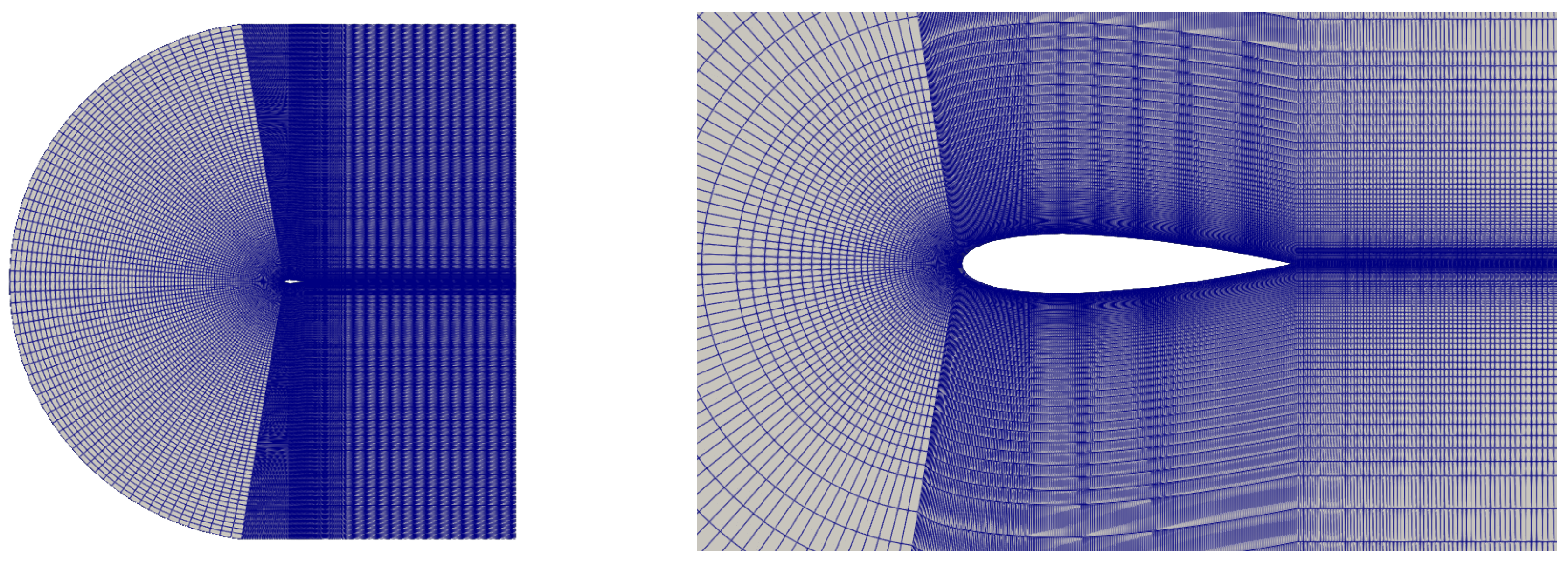
Figure 4 demonstrated that a grid with 198,000 cells is adequate for achieving a solution that is independent of grid size. This grid comprised 198,000 structured hexahedral cells, segmented into a far-field zone and a more detailed near-field region as shown in
Figure 5.
Multi-grading techniques were employed to modulate the cell expansion ratios within the blocks and enhance the refinement of the boundary layer adjacent to the airfoil wall. Furthermore, the aspect ratio of cells near the airfoil was meticulously managed to ensure they remained within acceptable ranges, given that cells with high aspect ratios, particularly in areas sensitive to flow, can sometimes compromise the reliability of the findings.
2.5. Solver Setup and Turbulence Model
The simulations were run using the steady-state Reynolds-Averaged Navier-Stokes (RANS) OpenFOAM ’simpleFOAM’ solver along with the viscous Spalart-Allmaras turbulence model. SimpleFOAM is a pressure-based solver (for low-speed incompressible flows) that incorporates the SIMPLE (Semi-implicit Method for pressure-linked equations) algorithm. This solver is generally preferred to other pressure-based OpenFOAM solvers (such as PisoFoam or PimpleFoam) for largely incompressible and turbulent flows around airfoils.
The Spalart-Allmaras model is a single-equation turbulence model, solving for the modified turbulent kinematic viscosity. It is widely used in various aerospace applications and is designed for low-velocity wall-bounding flows with boundary layers subject to adverse pressure gradients like in airfoils. It is commonly used for low-Reynolds number flows and is more straightforward to implement, unlike other turbulence models such as the k-
or the k-
models, which require the turbulent length scale to be calculated. The Spalart-Allmaras transport equation [
14], solving for the turbulent kinematic viscosity,
, is given below:
The turbulent viscosity,
can be determined through:
Subsequently, the viscous damping function,
is given by:
X represents the ratio of the turbulent kinematic viscosity to the kinematic viscosity:
The empirical constants for the Spalart-Allmaras model are given by: , , , , , , , , , .
The kinematic viscosity () for the domain is assumed to be . For the Spalart-Allmaras model, the turbulent viscosity () is initialized to be equal to the kinematic viscosity in the internal field of the domain, while the turbulent kinematic viscosity () is initialized to be equal to (X = 4).
2.6. Automation
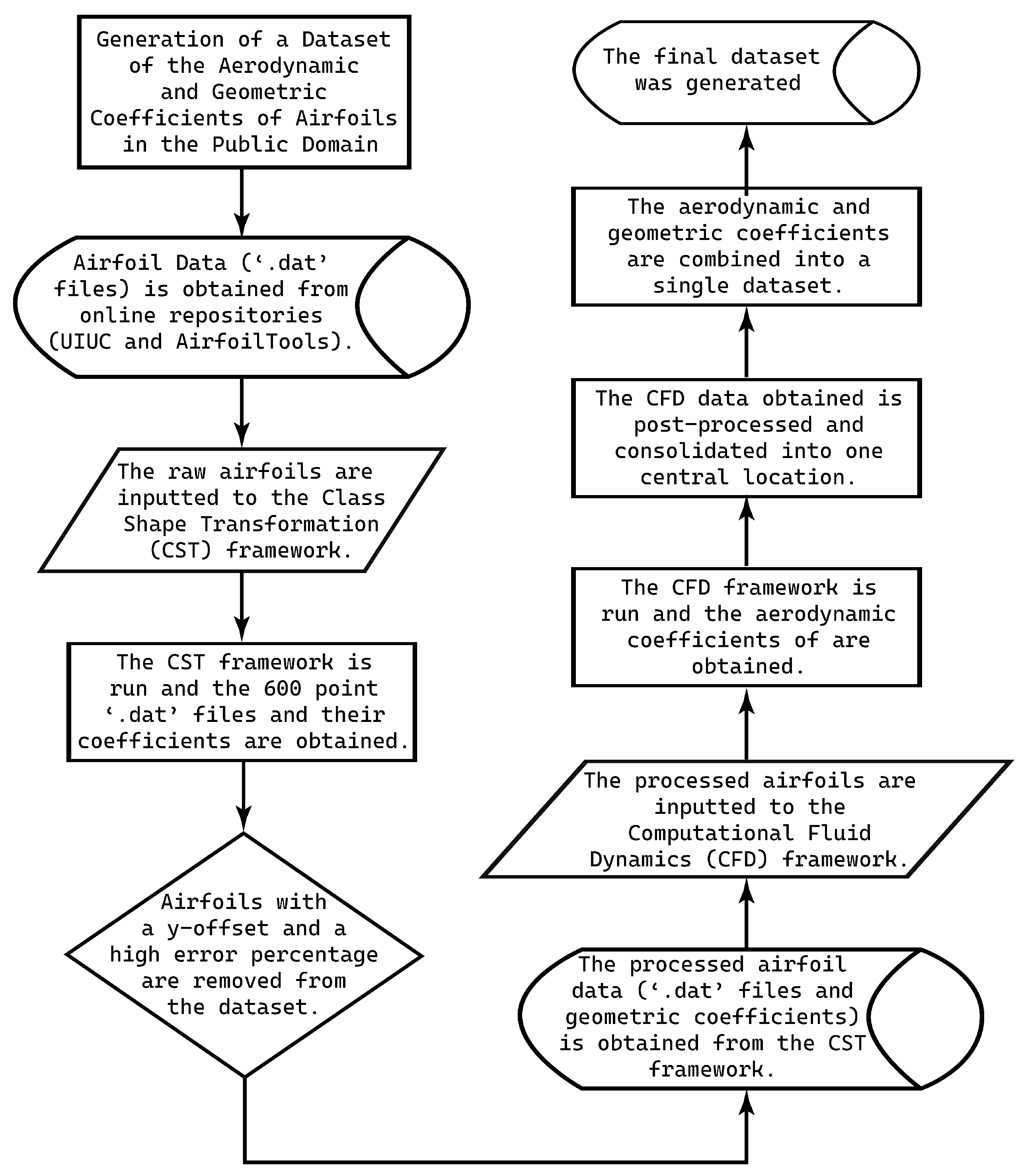
Automating the dataset creation process was a key component of the research. This was achieved through a comprehensive strategy. The software tools utilized for automation, listed in the order of their application, are illustrated in
Figure 6.
The CST framework was constructed utilizing MATLAB
®. Python played a key role in the automation of mesh creation. The execution of CFD simulations was streamlined through the use of Bash scripts. Additionally, Python was employed for the analysis and processing of the outcomes. The complete framework of the automation approach is illustrated in
Figure 7.
2.6.1. Automation of CST using MATLAB®
The automation of generating CST coefficients and the creation of 600-point ’.dat’ files was facilitated through MATLAB
®.
Figure 8 depicts the detailed procedure followed to accomplish this task.
2.6.2. Mesh Generation
Initially, a BlockMeshDict file conforming to a standard was developed to streamline the meshing process for airfoils. Following this, a Python script was crafted to retrieve coordinates from an airfoil ’.dat’ file and methodically replace them in the specified lines of the BlockMeshDict file. This approach enabled the efficient meshing of any Selig format ’.dat’ file with 600 points.
2.7. Bash Scripting
Bash scripts were pivotal in the research process, being utilized across various phases of the simulation, from initiating the case setup to managing the post-processing of the gathered results. Furthermore, they played a significant role in parallelizing the CFD simulations, controlling the numerous concurrent simulations.
2.7.1. CFD Automation
Multiple simulations indicated that 2000 iterations were enough to reach an almost converged solution, resulting in the final residuals for all parameters (U, p, and the turbulence parameters) being roughly around . Further, increasing the iteration count, which would significantly raise computational time and resources, did not affect the measured parameters. Therefore, in the process of automating the simulations, the iteration limit for each airfoil was set to 2000.
2.7.2. Parallelization
Throughout the study, OpenFOAM v2306 was the designated software version in use. The primary tool for simulation, the simpleFOAM solver, operates predominantly on a CPU. Initial simulations were conducted on a laptop equipped with a Ryzen 7 5800H CPU and 32 GB of RAM, featuring eight cores and 16 threads. Running a simulation on a single core took about 20 minutes, indicating that completing simulations for all the airfoils at a single angle of attack (AoA) would require approximately 42 days. This substantial time commitment led to the decision to implement parallel processing for the simulations.
Initially, parallel simulations were executed on the mentioned laptop before transferring the cases to a supercomputer powered by an AMD Epyc 32-core CPU with 110 GB of RAM. The airfoil database was divided, allowing for simultaneous runs of one case per sub-database. This setup ensured that several simulations were operational concurrently. The optimal number of simultaneous simulations was determined through experimentation, considering both the supercomputer’s performance and the cumulative simulation time for one AoA.
After fine-tuning the parallelization strategy, the ultimate simulations were carried out on four Intel Xeon Platinum Cascadelake 8268 processors, boasting a total of 96 cores and 1,536 GB of RAM. The database was segmented into 96 parts, leading to a final simulation time of approximately two days for one AoA.
2.7.3. Post-Processing
A Python script has been created to save the simulation outcomes, including the Angle of Attack (AoA) and the CST coefficients, in a CSV (Comma Separated Values) file. This approach was implemented to streamline the data consolidation process and facilitate subsequent data analysis.
3. Data Description
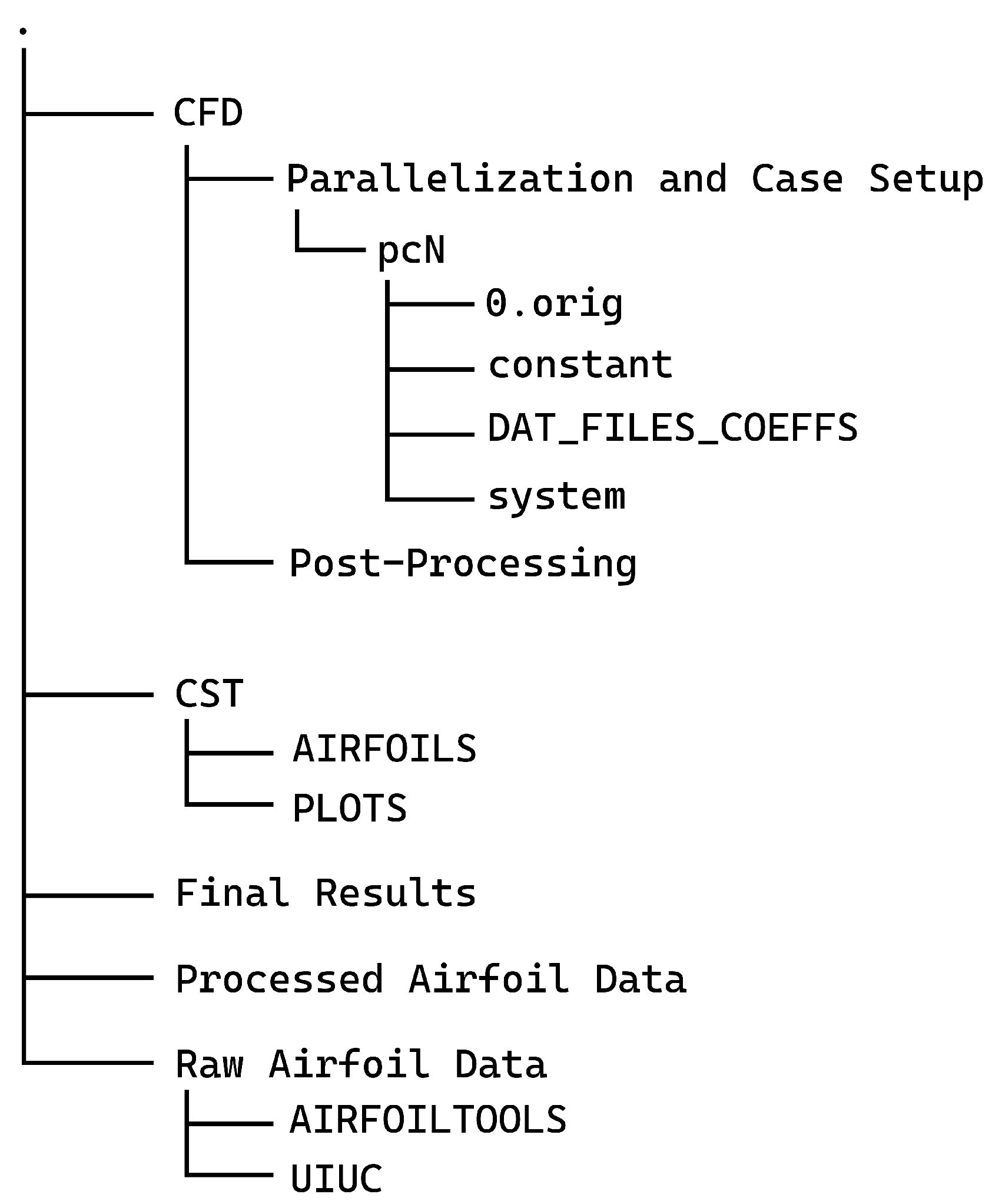
The dataset is stored on a GitHub repository. The data structure of the repository is shown in
Figure 9. The repository is primarily divided into five parts. These correspond to the raw and processed airfoil data, the CFD and CST subdirectories, and the final dataset. The CFD subdirectory contains the OpenFOAM case setup and its associated directories. Similarly, the CST subdirectory contains the CST framework. Further, separate directories have been created for the raw and processed airfoil databases.
The outcome of this study, the final dataset is provided in the following format represented in
Table 1,
Here, AoA refers to the angle of attack, the CST coefficients, and , are the lift and drag coefficients, respectively.
4. Data validation
The validation of lift and drag coefficients for selected symmetric and cambered airfoils was achieved by comparing the simulation results with experimental data cited from two distinct sources, focusing on a Reynolds number approximating 100,000. This process aimed to affirm the precision of both the outcomes and the simulation methodology itself, involving a comparison across various airfoil types. However, due to space limitations, only a select number of relevant illustrations are included. The validation for NACA airfoils utilized findings from the NACA report [
15], whereas validations for other non-NACA airfoils drew upon data from the data library [
16].
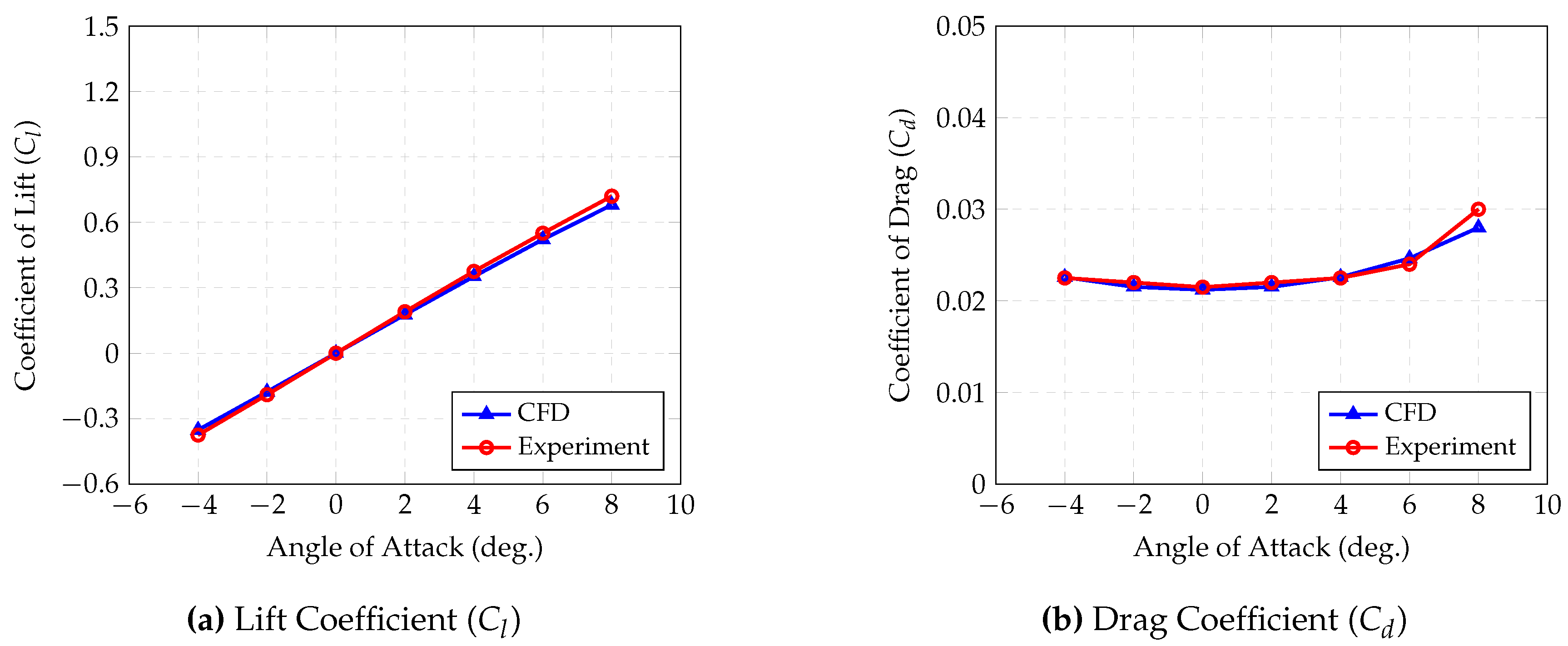
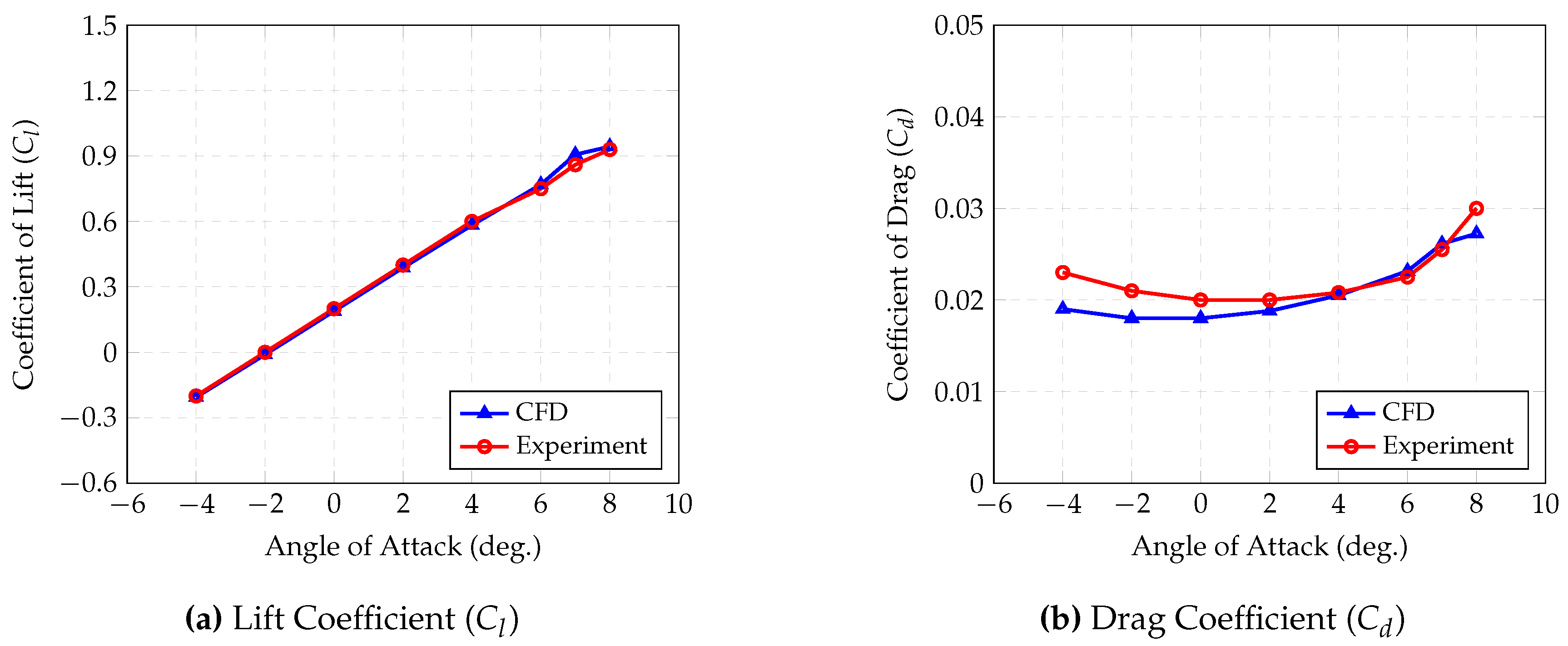
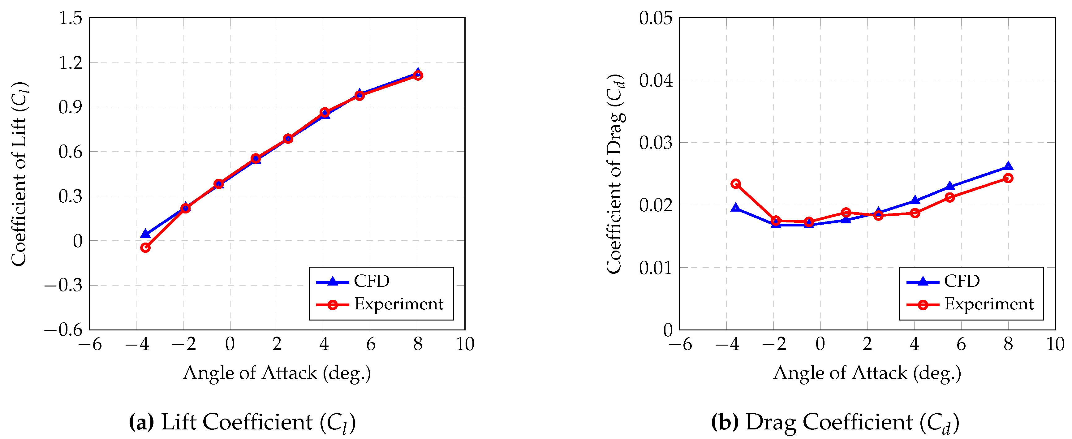
The comparison includes numerically derived and experimentally measured lift and drag coefficients for a symmetric airfoil, specifically the NACA 0018 at a Reynolds number of 84,000, and a cambered airfoil, the NACA 2412, at a Reynolds number of 82,800. For each airfoil, these comparisons are depicted in the designated
Figure 10 and
Figure 11.
The OpenFOAM model accurately predicts values within the selected range of angles of attack, paralleling experimental findings. The deviations for both lift and drag coefficients for the symmetric NACA 0018 airfoil fall below a 5% margin, indicating high precision in the results. Similarly, lift coefficient estimates for the cambered NACA 2412 airfoil align closely with experimental data, remaining within a 5% error margin. However, the model tends to underestimate the drag coefficients for the NACA 2412, showing a discrepancy of about 15% at certain angles of attack. This pattern is consistent across other tested airfoils, where lift coefficients are accurately predicted while drag coefficients are slightly underestimated.
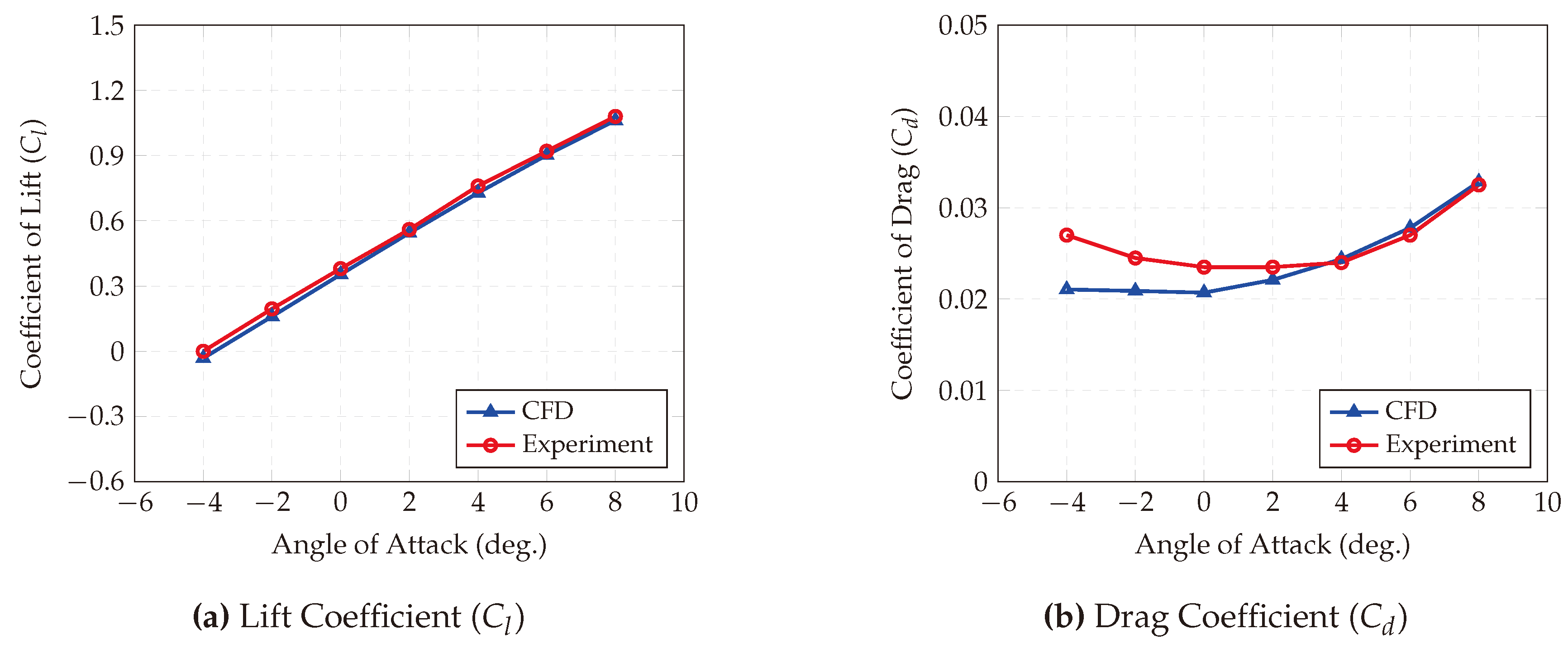
For the NACA 4415 and NACA 6412 airfoils at Reynolds numbers of 82,500 and 83,000, respectively, the results shown in
Figure 12 and
Figure 13 showcase that while lift coefficient (
) values are within a 5% error margin, the gap between predicted and experimental drag coefficient (
) values widens beyond 10% at both high and notably negative angles of attack.
Validation is also carried out for non-NACA airfoils. The results obtained for the Selig/Donnovan SD8020 airfoil at a Reynolds number of 101,800 is shown in
Figure 14. Expected results are obtained; the error in the lift is less than 4% while the error in the drag coefficient remains less than 10% apart from at highly negative angles of attack.
Predicting the aerodynamic performance, particularly drag, in scenarios of high flow separation or at significant angles of attack, poses a challenge for numerical methods [
17]. As the angle of attack reaches its limits, leading to detached flows, simulation results tend to deviate from those reported in literature. This deviation is challenging to address without resorting to unsteady Reynolds-Averaged Navier-Stokes (RANS) or Large Eddy Simulation (LES) techniques and the use of highly detailed meshes [
18]. Previous studies, including this one, have noted inconsistencies in the numerical versus experimental lift (
) and drag (
) coefficients across angles of attack (AoA) when employing the Spalart-Allmaras model [
19].
However, despite occasionally underestimating drag forces, the OpenFOAM numerical results provide adequate lift and drag estimations for the angles of attack required by our study, which do not involve predominant flow separation. Additionally, the high level of accuracy observed in simulations across various references further confirms the feasibility and effectiveness of the automated simulation processes.
5. Conclusions
This paper introduces a dataset featuring airfoil aerodynamic coefficients and CST parameters of airfoils obtained from reputable online repositories (the UIUC Airfoil Database and Airfoil Tools). Focused on low Reynolds numbers (100,000), it serves as a proof of concept of a robust and automated framework for CFD analyses. The release of both the CFD framework and dataset sets the stage for future research, including expansion to higher Reynolds numbers and the training of several AI models for low Reynolds number aerodynamic analyses. This dataset could serve as a valuable resource for researchers and engineers in various fields.
Author Contributions
Conceptualization, M.M.; Methodology, M.M., V.V., K.A., and D.M.; Software, V.V., K.A., and D.M.; Validation, V.V.; Automation, K.A. and D.M.; Data Collection, K.A.; Writing – Original Draft Preparation, V.V., K.A. and D.M.; Writing – Review & Editing, V.V., K.A., D.M. and M.M.; Visualization, K.A.; Supervision, M.M. All authors have read and agreed to the published version of the manuscript.
Funding
This research received no external funding.
Institutional Review Board Statement
Not applicable.
Informed Consent Statement
Not applicable.
Data Availability Statement
Acknowledgments
We would like to acknowledge the support of the Computer Science Engineering Department at the Manipal Institute of Technology, MAHE, Manipal, Karnataka, India. for giving us access to their supercomputer, "MIT Cloud GPU". We would also like to acknowledge the National Supercomputing Mission (NSM) for providing us with the computing resources of ‘PARAM UTKARSH’ at CDAC Knowledge Park, Bengaluru, Karnataka, India which is implemented by C-DAC and supported by the Ministry of Electronics and Information Technology (MeitY) and the Department of Science and Technology (DST), Government of India. We also acknowledge the support of the Aeronautical and Automobile Engineering Department at the Manipal Institute of Technology, MAHE, Manipal, Karnataka, India, for all their support along the way. We authors would like to thank Mr. Noble Sharma, Senior Application Engineer, Engine Systems, Gamma Technologies, Pune, India, for extending his support in performing the CFD analysis in OpenFOAM.
Conflicts of Interest
The authors declare no conflict of interest.
References
- Xiang, T.Z.; Xia, G.S.; Zhang, L. Mini-unmanned aerial vehicle-based remote sensing: Techniques, applications, and prospects. IEEE geoscience and remote sensing magazine 2019, 7, 29–63. [CrossRef]
- de Lucena, A.N.; da Silva, B.M.F.; Gonçalves, L.M.G. Micro aerial vehicle with basic risk of operation. Scientific Reports 2022, 12, 12772.
- Nex, F.; Remondino, F. UAV for 3D mapping applications: a review. Applied geomatics 2014, 6, 1–15. [CrossRef]
- Greening, B.; Azapagic, A. Environmental impacts of micro-wind turbines and their potential to contribute to UK climate change targets. Energy 2013, 59, 454–466. [CrossRef]
- Ribeiro, A.; Awruch, A.; Gomes, H. An airfoil optimization technique for wind turbines. Applied Mathematical Modelling 2012, 36, 4898–4907. [CrossRef]
- Li, J.; Zhang, M.; Tay, C.M.J.; Liu, N.; Cui, Y.; Chew, S.C.; Khoo, B.C. Low-Reynolds-number airfoil design optimization using deep-learning-based tailored airfoil modes. Aerospace Science and Technology 2022, 121, 107309. [CrossRef]
- Weller, H.G.; Tabor, G.; Jasak, H.; Fureby, C. A tensorial approach to computational continuum mechanics using object-oriented techniques. Computer in Physics 1998, 12, 620–631. [CrossRef]
- Kulfan, B.M. Universal parametric geometry representation method. Journal of aircraft 2008, 45, 142–158. [CrossRef]
- Selig, M. UIUC Airfoil Coordinates Database, Version 2.0, contains coordinates for approximately 1,600 airfoils. https://m-selig.ae.illinois.edu/ads/coord_database.html. [Online; accessed 03-March-2024].
- Airfoil Tools. http://www.airfoiltools.com/index. [Online; accessed 03-March-2024].
- Josh. http://www.joshtheengineer.com/2019/01/30/uiuc-airfoil-database-file-download/. [Online; Accessed 03-March-2024].
- Paula, A.A.d. The airfoil thickness effects on wavy leading edge phenomena at low Reynolds number regime. PhD thesis, Universidade de São Paulo, 2016.
- Pramudita Satria Palar. https://pramsatriapalar.wordpress.com/2017/02/24/how-to-fit-your-airfoil-with-cst-parameters/. [Online; Accessed 03-March-2024].
- Turbulence Modeling Resource. https://turbmodels.larc.nasa.gov/spalart.html#sa. [Online; Accessed 03-March-2024].
- Jacobs, E.N.; Sherman, A. Airfoil section characteristics as affected by variations of the Reynolds number. NACA Technical Report 1937, 586, 227–267.
- Selig, M.S. Summary of low speed airfoil data; SoarTech publications, 1995.
- Van Dam, C.P. Recent experience with different methods of drag prediction. Progress in Aerospace Sciences 1999, 35, 751–798. [CrossRef]
- Keane, A.J.; Sóbester, A.; Scanlan, J.P. Small unmanned fixed-wing aircraft design: a practical approach; John Wiley & Sons, 2017.
- Yang, L.; Zhang, G. Analysis of Influence of Different Parameters on Numerical Simulation of NACA0012 Incompressible External Flow Field under High Reynolds Numbers. Applied Sciences 2022, 12, 416. [CrossRef]
|
Disclaimer/Publisher’s Note: The statements, opinions and data contained in all publications are solely those of the individual author(s) and contributor(s) and not of MDPI and/or the editor(s). MDPI and/or the editor(s) disclaim responsibility for any injury to people or property resulting from any ideas, methods, instructions or products referred to in the content. |
© 2024 by the authors. Licensee MDPI, Basel, Switzerland. This article is an open access article distributed under the terms and conditions of the Creative Commons Attribution (CC BY) license (http://creativecommons.org/licenses/by/4.0/).
