Tuning of PID Controllers using Reinforcement Learning for Nonlinear Systems Control

1. Introduction

Despite the existence of a wide range of advanced control methods, most industrial processes use classical PID-type control laws as control methods. This is due to the robustness of these control laws to disturbances, to modeling errors or to the time variation of various parameters, but also due to the simplicity of implementation on both analog and digital devices.

Here are some specific examples of using PID controllers:

- In industrial processes, PID controllers are used to control temperature, pressure, level and other important variables. They can help keep these variables within safe and effective limits [1,2].

- In the aerospace industry, PID controllers are used to control the flight of aircraft. They can help keep the aircraft straight and on course, even in difficult conditions [3].

- In the automotive industry, PID controllers are used to control the engine, transmission, and other systems. They can help improve vehicle performance, efficiency and safety [4].

Tuning of classic PID controllers consists in setting the values of only three parameters - Kp, Ki and Kd - corresponding to the three actions specified in the name of these controllers - proportional (P), integrator (I), derivative (D). Although for linear systems the tuning of a PID controller is straightforward using various methods [5], the practical implementation raises numerous problems because real systems are non-linear (or the linearity zone is very narrow) or with variable parameters. Also, some processes allow aggressive controls while others require smooth controls. Thus, the selection of parameters must be carried out according to the specific characteristics of the process, which is why, in industrial practice, various approaches have been developed for tuning the parameters of PID controllers [6]. The simplest tuning method is trial and error. In this method, the parameters of the controller are adjusted according to the response of the system to various test signals. It is a method that requires experienced personnel and can lead to equipment failure if not performed carefully. Also, in this category of methods we can include tuning using the Ziegler – Nichols frequency response method [7]. In this case, the closed-loop system is brought to the stability limit and the parameters are adjusted based on practical rules. Another category of methods is based on obtaining a simplified first-order plus time delay model (FOPTD) and using preset tuning formulas to adjust the aggressiveness and robustness of the response to various types of input signals.

While PID controllers are particularly effective for linear systems, they can also be applied to certain nonlinear systems with some limitations. The challenge with nonlinear systems is that their behavior may vary across different operating points, and a fixed set of PID parameters may not provide optimal control across the entire range of system dynamics [8]. In some cases, nonlinearities can lead to instability or poor performance when using a standard PID controller.

However, there are several strategies to use PID controllers with nonlinear systems:

Linearization: One approach is to linearize the system around an operating point and design a PID controller for that linearized model. This can work well if the nonlinearities are relatively small within the operating range.

Gain Scheduling: Another method is gain scheduling, where different sets of PID parameters are used for different operating conditions or operating points in the system's state space. The controller parameters are adjusted based on the system's nonlinearities.

Adaptive Control: Adaptive control techniques can be employed to adjust the PID parameters online based on the changing characteristics of the nonlinear system. This requires a feedback mechanism to continuously update the controller parameters.

This paper presents a method based on Machine Learning for tuning the parameters of PID controllers for automatic control of some classes of nonlinear systems. The development of machine learning methods in the field of artificial intelligence did not remain without an echo in the field of process control. Thus, the most well-known algorithms in the field of Reinforcement Learning (the field of AI closest to automatic control) have been tested and implemented in applications of control systems [9,10]. In particular, the actor-critic methods in RL have been intensively used for systems control and optimization problems. Reinforcement learning (RL) is a type of machine learning where an agent learns to behave in an environment by trial and error. The agent receives rewards for taking actions that lead to desired outcomes, and punishments for taking actions that lead to undesired outcomes. Over time, the agent learns to take actions that maximize its rewards. RL is a powerful technique that can be used to solve a wide variety of problems, including game playing, robotics, and finance [11].

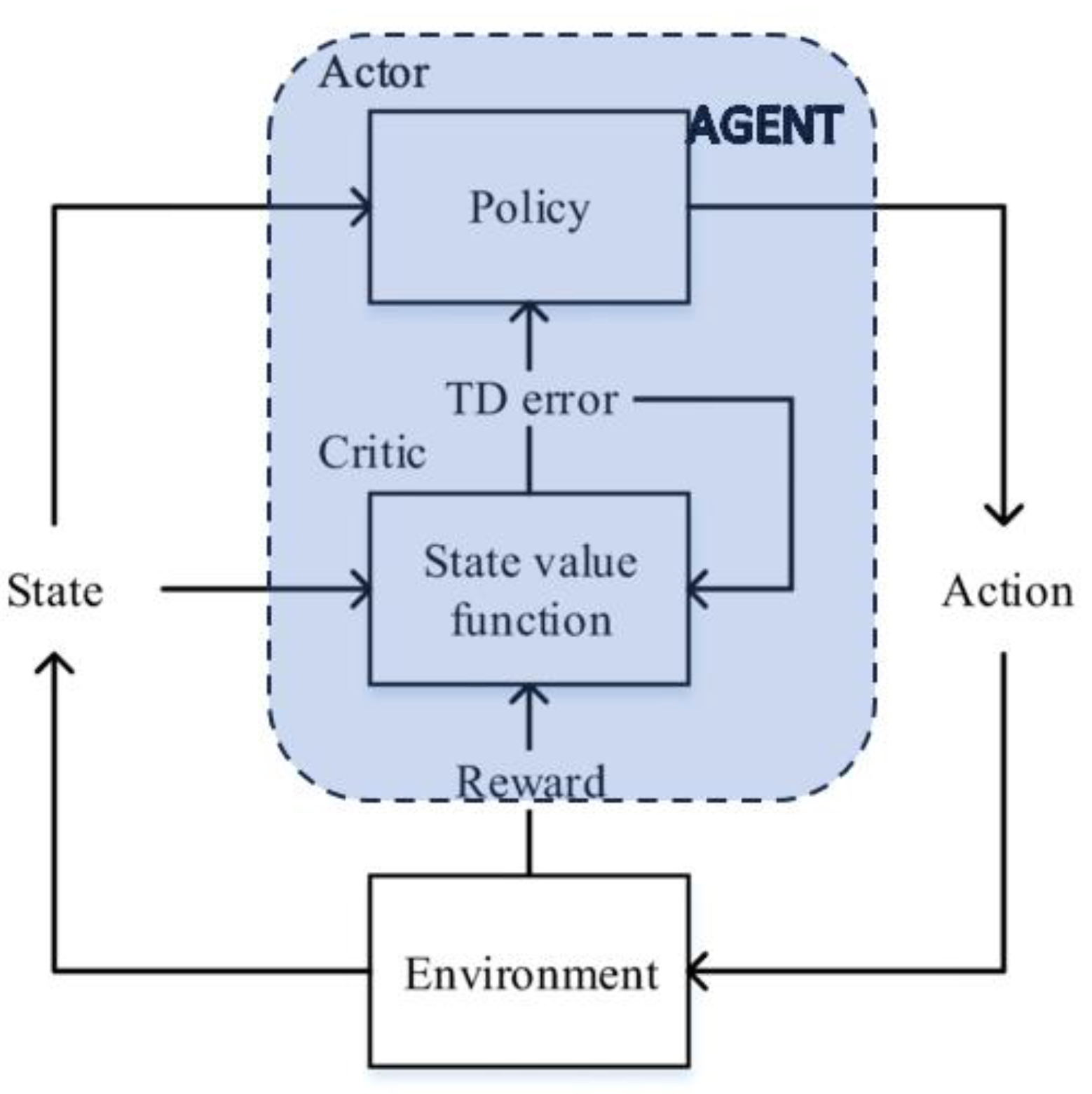
RL is a challenging field of machine learning, but it is also one of the most promising. RL has the potential to solve problems that are beyond the reach of other machine learning techniques. Some of the key concepts in reinforcement learning are the following (see also Figure 1):

• Agent: The agent is the entity that is learning to behave in an environment. The most common structure for the agent is composed of two elements: Critic and Actor. The critic estimates the expected cumulative reward (value) associated with being in a certain state and following the policy defined by the actor. The actor is responsible for learning and deciding the optimal policy – the mapping from states to actions. It is essentially the decision-maker or policy function.
• Environment: The environment is the world that the agent interacts with.
• State: The state is the current condition of the environment.
• Action: An action is something that the agent can do in the environment.
• Reward: A reward is a signal that indicates whether an action was good or bad.
• Policy: A policy is a rule that tells the agent what action to take in a given state.
• Value function: A value function is a measure of how good it is to be in a given state.

The basic idea of RL-type algorithms is to improve their policy, and, from this point of view, two main approaches have been developed: on-policy and off-policy learning. On-policy and off-policy are two categories of reinforcement learning algorithms that differ in how they use collected data for learning. The key distinction lies in whether the learning policy (the policy being optimized) is the same as the policy used to generate the data [12]. In on-policy algorithms, the learning agent follows a specific policy while collecting data, and this policy is the one being improved over time (the data used for learning (experience) comes from the same policy that is being updated). In off-policy algorithms, the learning agent has its own exploration policy for collecting data, but it learns and improves a different target policy (the data used for learning can come from a different (possibly older) policy than the one being updated). Representative examples are SARSA (State-Action-Reward-State-Action) for on-line learning and Q-learning for off-line learning.

Reinforcement learning algorithms for continuous states have evolved significantly over the years, driven by the need to address real-world problems with continuous and high-dimensional state spaces. The early days of RL were dominated by discrete state and action spaces. Dynamic programming algorithms, such as the Bellman equation, were effective for solving problems with small, discrete state spaces. However, they were not suitable for continuous spaces due to the curse of dimensionality. To handle continuous states, researchers introduced function approximation techniques. Value function approximation using methods like tile coding and coarse coding helped extend RL to continuous state spaces. This approach laid the foundation for handling larger and more complex state representations. Policy gradient methods emerged as an alternative to value-based approaches. Instead of estimating the value function, these methods directly learn a parameterized policy. Algorithms like REINFORCE and actor-critic methods became popular for problems with continuous state and action spaces.

They are particularly effective when dealing with high-dimensional and complex problems. The advent of deep neural networks brought about a revolution in RL. Deep Q-Networks (DQN) extended RL to problems with high-dimensional state spaces, and later algorithms like Deep Deterministic Policy Gradients (DDPG) and Trust Region Policy Optimization (TRPO) addressed continuous action spaces. These methods leverage neural networks to approximate complex mappings from states to actions.

Twin Delayed DDPG (TD3) is an off-policy reinforcement learning algorithm designed for continuous action spaces. It is an extension of the Deep Deterministic Policy Gradients (DDPG) algorithm with several modifications to enhance stability and performance. TD3 was introduced by Scott Fujimoto et al. 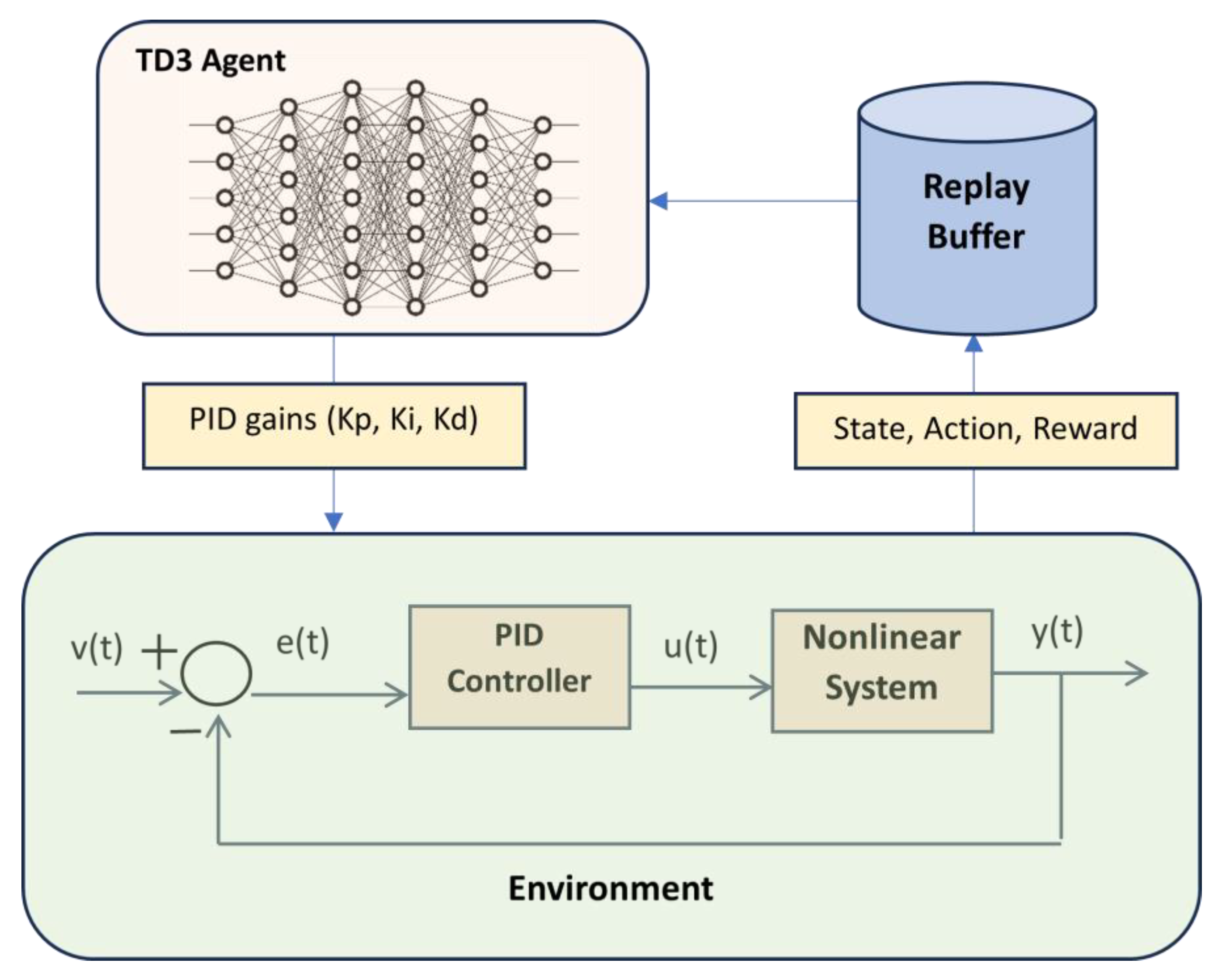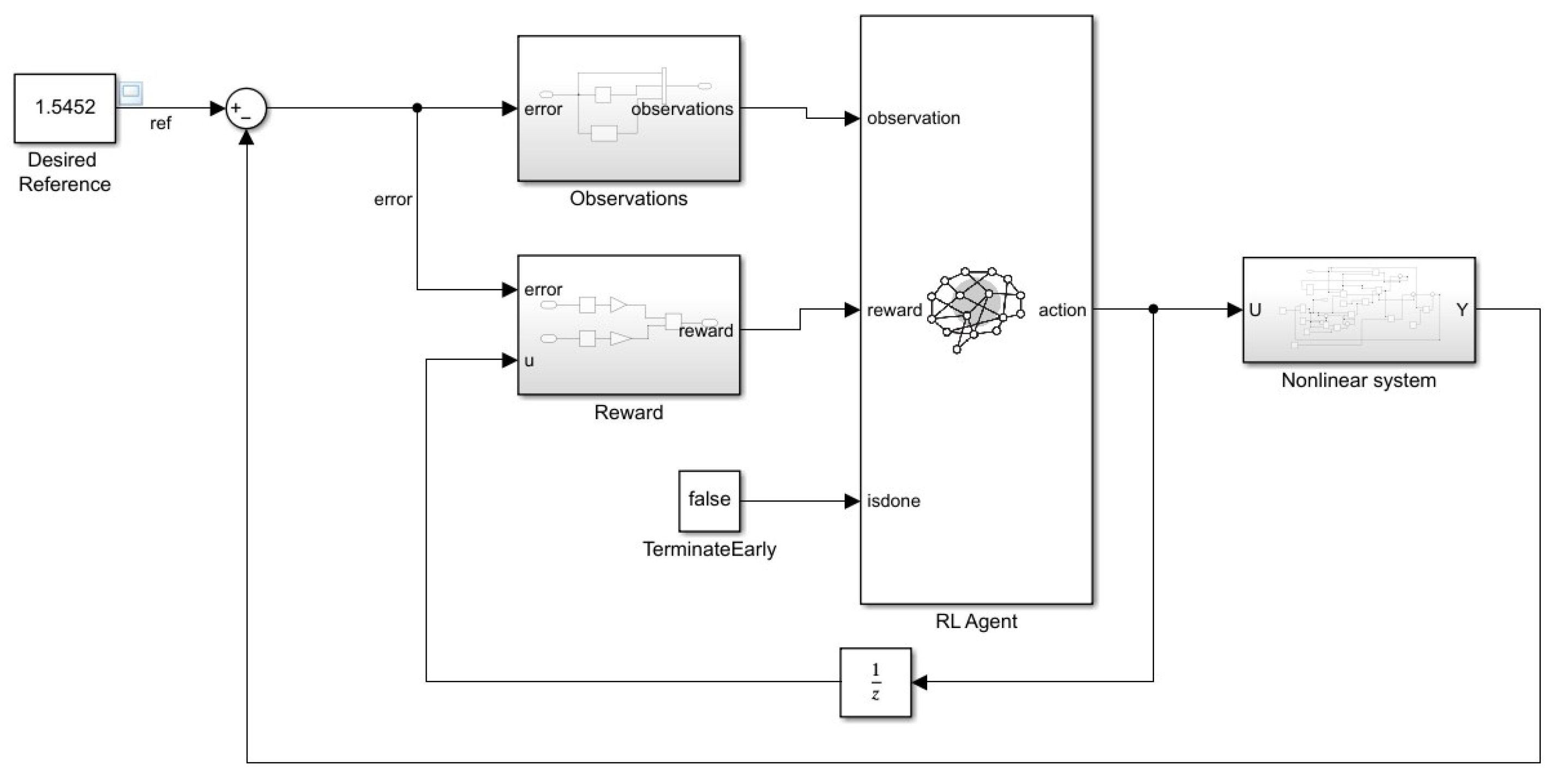in their 2018 paper titled “Addressing Function Approximation Error in Actor-Critic Methods” [13] and has been successfully used in several control applications [14]. In this paper, the TD3 algorithm was used to tune the parameters of the PID controller from a control loop of a nonlinear system.

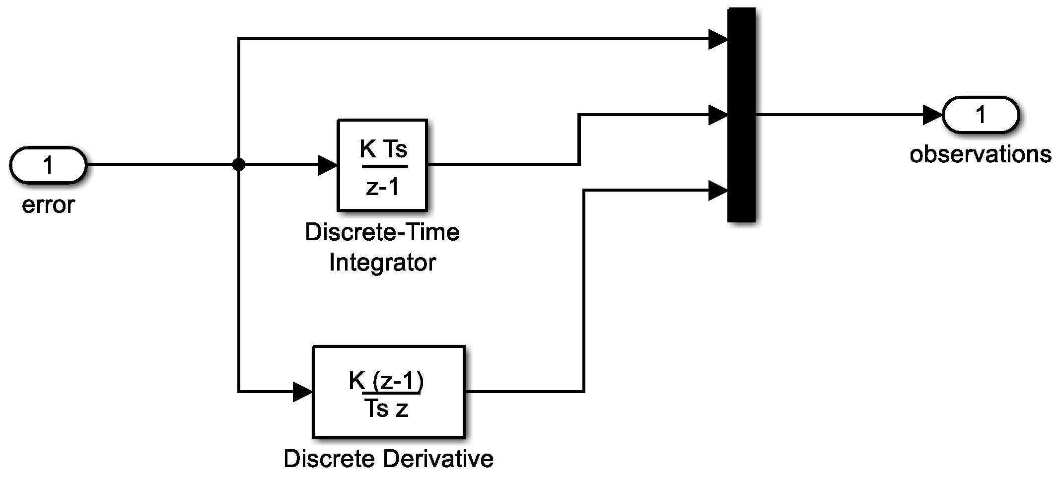
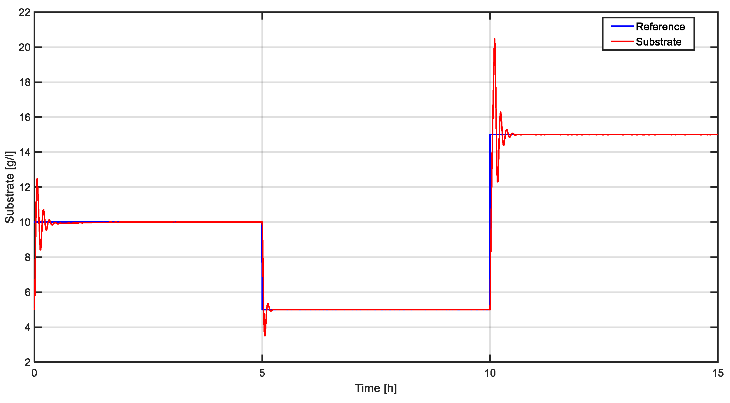
Next, the paper is structured as follows: in Section 2 the TD3 algorithm is presented in detail, Section 3 presents the tuning of the PID controller parameters using the TD3 algorithm, in Section 4 presents the classical approach of PID tuning for a nonlinear system, Section 5 presents the simulation results of the two approaches and Section 6 is dedicated to the conclusions regarding the results obtained and possible future approaches.

2. Twin Delayed Deep Deterministic Policy Gradient (TD3) Algorithm

TD3 (Twin Delayed Deep Deterministic Policy Gradient) is an off-policy actor-critic reinforcement learning algorithm. It is a successor (an enhanced version) to the Deep Deterministic Policy Gradient (DDPG) algorithm, and it addresses some of the shortcomings of DDPG, such as overestimation bias and numerical instability. Since TD3 is built on DDPG with some modifications, we will present the DDPG algorithm first.

2.1. Deep Deterministic Policy Gradient

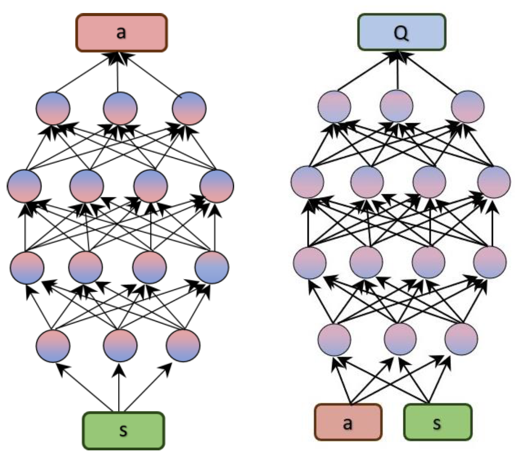
The main elements of DDPG and TD3 algorithms are represented by two types of deep neural networks: actor neural network and critic neural network [14]. The general structure of these networks is shown in Figure 2. The actor is associated with policy-based methods. It can learn a policy that maps states in the environment to actions, trying to find an optimal policy that maximizes long-term rewards. The actor network receives as input the state of the environment and has as output the action to be applied in that state.

The critic estimates the value function of the states or of the pairs (state, action) in the environment. The value function indicates how much reward you are expected to get by starting from a certain state and taking a certain action. The critic evaluates actions taken by the actor in a given environment and provides feedback regarding how well those actions performed in achieving desired goals or rewards. The most used technique for establishing the value function is Q-learning. In Q-learning, a function (usually denoted Q) that associates state-action pairs with the expected value of the future reward is estimated using a deep neural network.

In the following, we shall use the usual notations from RL, presented in Table 1.

DDPG is an actor-critic algorithm that presents the advantages of both policy-based and value-based methods and learn optimal estimates of both policy and value function. Using Bellman equation and off-policy data the Q-function is learnt and then is used to learn the policy [15]. The main idea is the same from Q learning: if the optimal Q-function (denoted $Q^{opt}(s,a)$) is known, the optimal action is obtained solving the following equation:

$$a^{opt}\left(s\right)=arg\underset{a}{\max }{Q}^{opt}(s,a),$$

(1)

The starting point in learning an approximator for $Q^{opt}(s,a)$ is the well-known Bellman equation:

$$Q^{opt}\left(s_k,a_k\right)=\mathbb{E}\left[r_k+\gamma \underset{a\in \mathbb{A}}{\max }{Q}^{opt}\left(s_{k+1},a\right)\right],$$

(2)

Q-learning solves the Bellman optimality equation using temporal difference (TD):

$$Q\left(s_k,a_k\right)\leftarrow Q\left(s_k,a_k\right)+\alpha \left[r_k+\gamma \underset{a\in \mathbb{A}}{\max }Q\left(s_{k+1},a\right)-Q\left(s_k,a_k\right)\right],$$

(3)

where

• $\delta =\left[r_k+\gamma \underset{a\in \mathbb{A}}{\max }Q\left(s_{k+1},a\right)-Q\left(s_k,a_k\right)\right]$ – TD-error
• $\alpha$ – learning rate

In order to use Q-learning for continuous state and action spaces, neural networks were used as function approximators for Q values and function policy. So, considering $Q_w$ - critic network parametrized by w and ${\pi }_{\theta }$ - actor network parametrized by θ, relation (3) becomes:

$$Q_w\left(s_k,a_k\right)\leftarrow Q_w\left(s_k,a_k\right)+\alpha \left[r_k+\gamma \underset{a\in \mathbb{A}}{\max }{Q}_w\left(s_{k+1},a\right)-Q_w\left(s_k,a_k\right)\right],$$

(4)

In relation (4) the term ${{\phi }_k=r}_k+\gamma \underset{a\in \mathbb{A}}{\max }{Q}_w\left(s_{k+1},a\right)$ represents the target (the desired or goal value that the algorithm is trying to approximate or learn). The target ${\phi }_k$ depends on the parameter w that is to be optimized so, the target is varying and this causes significant difficulty for the supervised learning. The solution to this problem in DDPG was to use a new neural network (called critic target network) that has a similar structure with the critic network but whose parameters does not change rapidly. Also, the target ${\phi }_k$ contains the maximization over $a\in \mathbb{A}$ that can be expensive since the Q value function is a complex network with continuous inputs. To address this problem, a target actor network is used to approximate the optimal policy that maximizes $Q_w\left(s_{k+1},a\right)$. The target networks are denoted in the following by:

${\widehat{Q}}_{\widehat{w}}$ - target critic network parametrized by $\widehat{w}$

${\widehat{\pi }}_{\widehat{\theta }}$ - target actor network parametrized by $\widehat{\theta }$

So, the target becomes:

$${{\phi }_k=r}_k+\gamma ·{\widehat{Q}}_{\widehat{w}}(s_{k+1},{\widehat{\pi }}_{\widehat{\theta }}\left(s_{k+1}\right)),$$

(5)

For training the critic $Q_w$, using a minibatch of N samples and a target critic ${\widehat{Q}}_{\widehat{w}}$, compute

$${{\phi }_i=r}_i+\gamma ·{\widehat{Q}}_{\widehat{w}}(s_{i+1},{\widehat{\pi }}_{\widehat{\theta }}\left(s_{i+1}\right)),$$

(6)

and update w by minimizing the loss function L_C (calculated as the mean square error (MSE) between the current Q-value and the target Q-value):

$$L_c=\frac{1}{N}{\sum }_i{({\phi }_i-Q_w(s_i,a_i\left)\right)}^2,$$

(7)

In order to update the actor network parameters, the policy gradient is used:

$${\nabla }_{\theta }J=\frac{1}{N}{\sum }_i\left({\nabla }_a{Q}_w\right(s_i,a_i\left){·\nabla }_{\theta }{\pi }_{\theta }\right(s_i\left)\right),$$

(8)

For updating the target network parameters, DDPG performs “soft updates” using Polyak averaging:

$$\begin{array}{c}\widehat{w}\leftarrow \tau ·w+(1-\tau )·\widehat{w}\\ \widehat{\theta }\leftarrow \tau ·\theta +(1-\tau )·\widehat{\theta }\end{array},$$

(9)

where $\tau \in \left[0,1\right],\tau \ll 1$.

In summary, the main steps of the DDPG algorithm are:

1. Initialize the critic and actor networks.

2. Collect data from the environment and store them in the replay buffer.

3. Sample a batch of experiences from the replay buffer.

4. Compute the target Q-value using the target networks and update the critic using a mean-squared Bellman error loss.

5. Update the actor policy using the sampled batch, aiming to maximize the estimated Q-value.

6. Periodically update the target networks with a soft update.

7. Repeat steps 3-6 until the desired performance is achieved.

2.2. TD3 – The Main Characteristics

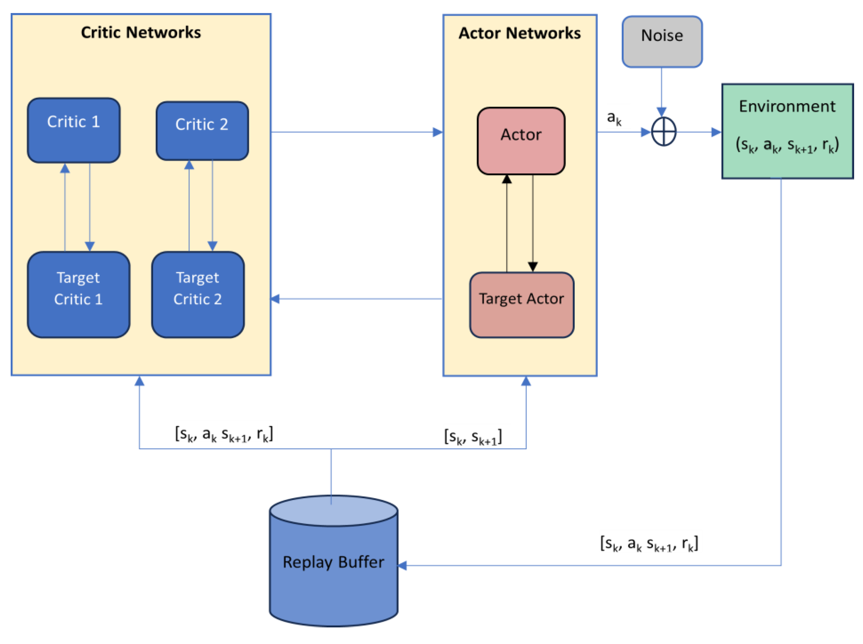
In Figure 3 is presented the general structure of TD3 algorithm. There are used six neural networks, namely, two critics, two critic targets, an actor and corresponding target. During each interaction with the environment, the agent collects experiences in the form of tuples (state, action, reward, next state). Instead of immediately using these experiences to update the policy or value function, the experiences are stored in the replay buffer. The replay buffer is a mechanism used in DDPG and TD3 to store and replay past experiences, promoting more stable and efficient learning in continuous action space reinforcement learning problems. A replay buffer is a key component used to store and sample experiences from the agent's interactions with the environment. The replay buffer typically has a fixed size, and new experiences overwrite the oldest ones once the buffer is full. This ensures a continuous flow of new experiences while still benefiting from historical data. Training a neural network with sequential experiences can lead to high correlations between consecutive samples, which may hinder learning. The replay buffer allows for random sampling of experiences, breaking the temporal correlations and providing more diverse training data.

Overconfidence bias (a term that comes from psychology), defines a disparity between one's self-assessment of skills and abilities and the actual reality. This phenomenon extends beyond human behavior and is prevalent among RL agents, known in RL terminology as "Overestimation Bias." Another drawback of Q-learning algorithms is the possible numerical instability generated using function approximation to estimate Q-values for continuous or large state-action spaces. Instabilities can arise when training neural networks, especially if they are deep. Issues like vanishing gradients or exploding gradients can affect the stability of the learning process. Consequently, the TD3 algorithm was developed to address these challenges within the Actor-Critic RL framework, specifically targeting the limitations observed in the DDPG algorithm. TD3 concentrates specifically on the Actor-Critic framework, implementing three techniques to enhance the DDPG algorithm: 1. Clipped Double Q-Learning, 2. Target policy smoothing and 3. Delayed policy and target updates.

Clipped double Q-learning is a way of reducing overestimation bias in the Q-functions. Double Q-learning addresses the overestimation problem by using two sets of Q-values (Q₁ and Q₂), and during the updates, it uses one set to select the best action and the other set to evaluate that action [16]. Clipped Double Q-learning goes a step further by introducing a clipping mechanism during the Q-value updates (as summarized in Figure 4). The idea is to prevent overestimation by limiting the impact of the maximum estimated Q-value.

When updating Q-values, the algorithm compares the Q-values from the two sets and chooses the smaller one. This clipped value is then used in the update rule. Since only a single actor π is used, a single TD-Target is then used for updating both Q₁ and Q₂.

$${{\phi }_k=r}_k+\gamma ·min\left\{{\widehat{Q}}_{\widehat{w}1}(s_{k+1},{\widehat{\pi }}_{\widehat{\theta }}\left(s_{k+1}\right),{\widehat{Q}}_{\widehat{w}2}(s_{k+1},{\widehat{\pi }}_{\widehat{\theta }}\left(s_{k+1}\right)\right\},$$

(10)

Target policy smoothing is a way of making the updates to the policy less aggressive. This helps to prevent the policy from diverging too far from the current policy, which can lead to instability. In order to prevent that, a perturbation $\eta$ (usually chosen as a small Gaussian noise) is added to the action of the next state, so that the value evaluation is more accurate. Additionally, the noise itself, as well as the perturbed action are clipped. The noise is clipped to ensure that it applies to only a small region around the action, while the perturbed action is clipped to ensure that it lies within the range of valid action values.

$${{\phi }_k=r}_k+\gamma ·min\left\{{\widehat{Q}}_{\widehat{w}1}(s_{k+1},{\widehat{\pi }}_{\widehat{\theta }}\left(s_{k+1}\right),{\widehat{Q}}_{\widehat{w}2}(s_{k+1},{\widehat{\pi }}_{\widehat{\theta }}\left(s_{k+1}\right)\right\}+\eta ,$$

(11)

where $\eta \sim clip(N\left(0,\sigma \right),-c,c)$.

So, the update of w₁ and w₂ (critics parameters) is realized by minimizing two loss functions:

$$\begin{array}{c}{L}_{c1}=\frac{1}{N}\sum _i{({\phi }_i-Q_{w1}(s_i,a_i\left)\right)}^2\\ L_{c2}=\frac{1}{N}\sum _i{({\phi }_i-Q_{w2}(s_i,a_i\left)\right)}^2\end{array},$$

(12)

Delayed policy and target updates is a technique by which the target networks are updated less often than the main networks. In TD3, the policy update is delayed. Instead of updating the policy every time step, the policy network is updated less frequently, typically after a fixed number of iterations or time steps. This delay helps in reducing the correlation between consecutive policy updates, leading to more stable learning and better exploration of the action space. In addition to delaying the policy updates, TD3 also introduces delayed updates to the target networks (both the actor and the critic networks). In DDPG, the target networks are updated by directly copying the weights from the main networks periodically. However, in TD3, the target networks are updated less frequently than the main networks. Specifically, the target networks are updated less often than the policy network updates. This delayed updating of the target networks helps in stabilizing the learning process by providing more consistent target values for the temporal difference (TD) error calculation, thus reducing the variance in the update process. These two strategies, delayed policy updates and delayed target updates, work together to improve the stability and performance of the TD3 algorithm, making it more effective in training deep reinforcement learning agents for complex tasks. Similar to DDPG, we used Polyak averaging technique with the formula below (τ has a very small value):

$$\begin{array}{c}{\widehat{w}}_1\leftarrow \tau ·w_1+(1-\tau )·{\widehat{w}}_1\\ {\widehat{w}}_2\leftarrow \tau ·w_2+(1-\tau )·{\widehat{w}}_2\\ \widehat{\theta }\leftarrow \tau ·\theta +\left(1-\tau \right)·\widehat{\theta }\end{array},$$

(13)

TD3 is a complex algorithm, but it is relatively easy to implement. Summarizing the above, the TD3 algorithm is as follows [18]:

Algorithm - TD3:

1. Initialize critic networks $Q_{w1}$, $Q_{w2}$, and actor network ${\pi }_{\theta }$ with random parameters $w_1$, $w_2$, $\theta$.

2. Initialize the parameters of target networks:

$${\widehat{w}}_1{\leftarrow w}_1$$

3. Initialize replay buffer B

for k= 1 to T do

4.Select action with exploration noise $a\leftarrow {\pi }_{\theta }+\eta$ and observe reward r_k and new state s_k+1

5. Store transition (s_k, a_k , s_k+1, r_k) in B

6. Sample mini-batch of N transitions (s_k, a_k, s_k+1, r_k) from B and compute

$$\begin{gathered} a_k\leftarrow {\widehat{\pi }}_{\widehat{\theta }}\left(s_{i+1}\right)+\eta \\ \eta \leftarrow clip(N\left(0,\sigma \right),-c,c) \\ {{\phi }_k\leftarrow r}_k+\gamma ·min\left\{{\widehat{Q}}_{\widehat{w}1},{\widehat{Q}}_{\widehat{w}2}\right\}+\eta \end{gathered}$$

7. Update critics parameters:

$$w_1\leftarrow arg\underset{w1}{\min }\frac{1}{N}\sum {({\phi }_k-Q_{w1}(s_k,a_k\left)\right)}^2{w}_2\leftarrow arg\underset{w2}{\min }\frac{1}{N}\sum {({\phi }_k-Q_{w2}(s_k,a_k\left)\right)}^2$$

8. Update $\theta$ by the deterministic policy gradient

$${\nabla }_{\theta }J=\frac{1}{N}\sum _i\left({\nabla }_a{Q}_{w1}\right(s_k,a_k\left){·\nabla }_{\theta }{\pi }_{\theta }\right(s_k\left)\right)$$

9. Update target networks:

$$\begin{gathered} {\widehat{w}}_1\leftarrow \tau ·w_1+(1-\tau )·{\widehat{w}}_1 \\ {\widehat{w}}_2\leftarrow \tau ·w_2+(1-\tau )·{\widehat{w}}_2 \\ \widehat{\theta }\leftarrow \tau ·\theta +(1-\tau )·\widehat{\theta } \end{gathered}$$

end for

3. Tunning of PID Controllers Using TD3 Algorithm

In the following, we will consider a standard PID type controller with the following input – output relation:

$$u=\left[\begin{array}{cc}e& \int edt\frac{de}{dt}\end{array}\right]\ast {\left[\begin{array}{cc}Kp& KiKd\end{array}\right]}^T,$$

(18)

Here:

• u is the output of the actor neural network.
• Kp, Ki and Kd are the PID controller parameters.
• e(t)=v(t)−y(t) where e(t) is system error, y(t) is the system output, and v(t) is the reference signal.

The proposed control structure with tuning of the PID controller parameters using the TD3 algorithm is presented in Figure 5. Given observations, a TD3 agent decides which action to take using an actor representation. The weights of the actor are, in fact, the gains of the PID controller so, one can model the PID controller as a neural network with one fully-connected layer with error, error integral and error derivative as inputs (state of the system). The output of the actor neural network represents the command signal (action). The proposed scheme has two time scales: a scale for adapting the PID controller parameters (the weights of the actor) and a scale for analyzing the system's response to a step input.

The reward can be defined using point-based metrics (e.g. settling time, overshoot etc.) or metrics based on system trajectory. In our study one used a reward function based on LQG criterion (see Section 5).

4. Tuning PID Controller for a Biotechnological System – Classical Approach

Designing a PID controller for biotechnological processes is a difficult task because, in general, these processes are very slow (usually the time constants of the system are measured in hours), in many cases unstable, which makes practical tuning methods (for example Ziegler-Nichols type methods) impossible to apply. For these reasons, to design a PID controller for a biotechnological process, it is necessary first to obtain a linearized model after which various tuning methods can be applied [17]. We present below the procedure for obtaining a linearized model for a bacterial growth biosystem around an operating point. Modelling of bioprocesses that take place in a fed-batch bioreactor is based on the general mass-balance equations [18]. Starting from these equations, the general model is represented by a set of nonlinear differential equations of the following form:

$$\dot{\xi }\left(t\right)=f\left(\xi ,D,F\right)=\mathsf{\Gamma }\cdot \Phi (\xi ,t)-D\xi \left(t\right)+F\left(t\right),$$

(19)

where:

• $\xi \left(t\right)\in {\mathfrak{R}}^{n\times 1}$ - represents the state vector (the concentrations of the systems variables);
• $\Phi ={\left[\begin{array}{cccc}{\mu }_1& {\mu }_2& \cdots & {\mu }_m\end{array}\right]}^T$ - denotes the vector of reactions kinetics (the rates of the reactions);
• $\mathsf{\Gamma }=\left[{\gamma }_{ij}\right],$ $i=\overline{1,n};j=\overline{1,m}$, is the matrix of the yield coefficients;
• $\mathsf{\Gamma }\cdot \Phi (\xi ,t)$ represents the rate of production;
• $-D\xi \left(t\right)+F\left(t\right)$ is the exchange between the bioreactor and the exterior.

This model is strongly non-linear, a specific characteristic of most biotechnological processes. In order to design a PID controller the system represented by relation (19) could be linearized around of an equilibrium point $\left(\tilde{\xi },\tilde{D},\tilde{F}\right)$ (that is a solution of the equation $f\left(\xi ,D,F\right)=0)$. One gets the following equations:

$$\frac{d}{dt}\left(\xi -\tilde{\xi }\right)=A\left(\tilde{\xi }\right)\cdot \left(\xi -\tilde{\xi }\right)-\left(D-\tilde{D}\right)\tilde{\xi }+\left(F-\tilde{F}\right),$$

(20)

with

$$A\left(\tilde{\xi }\right)=\mathsf{\Gamma }·{\left[\frac{\partial \Phi \left(\xi \right)}{\partial \xi }\right]}_{\xi =\tilde{\xi }}-\tilde{D}{I}_2,$$

(21)

where $\tilde{\xi }$ represents the equilibrium value of $\xi$ and I₂ represents the second order unity matrix. The linear model (20) – (21) can be used to tune the PID parameters using classical design formulas or computer aided design approaches.

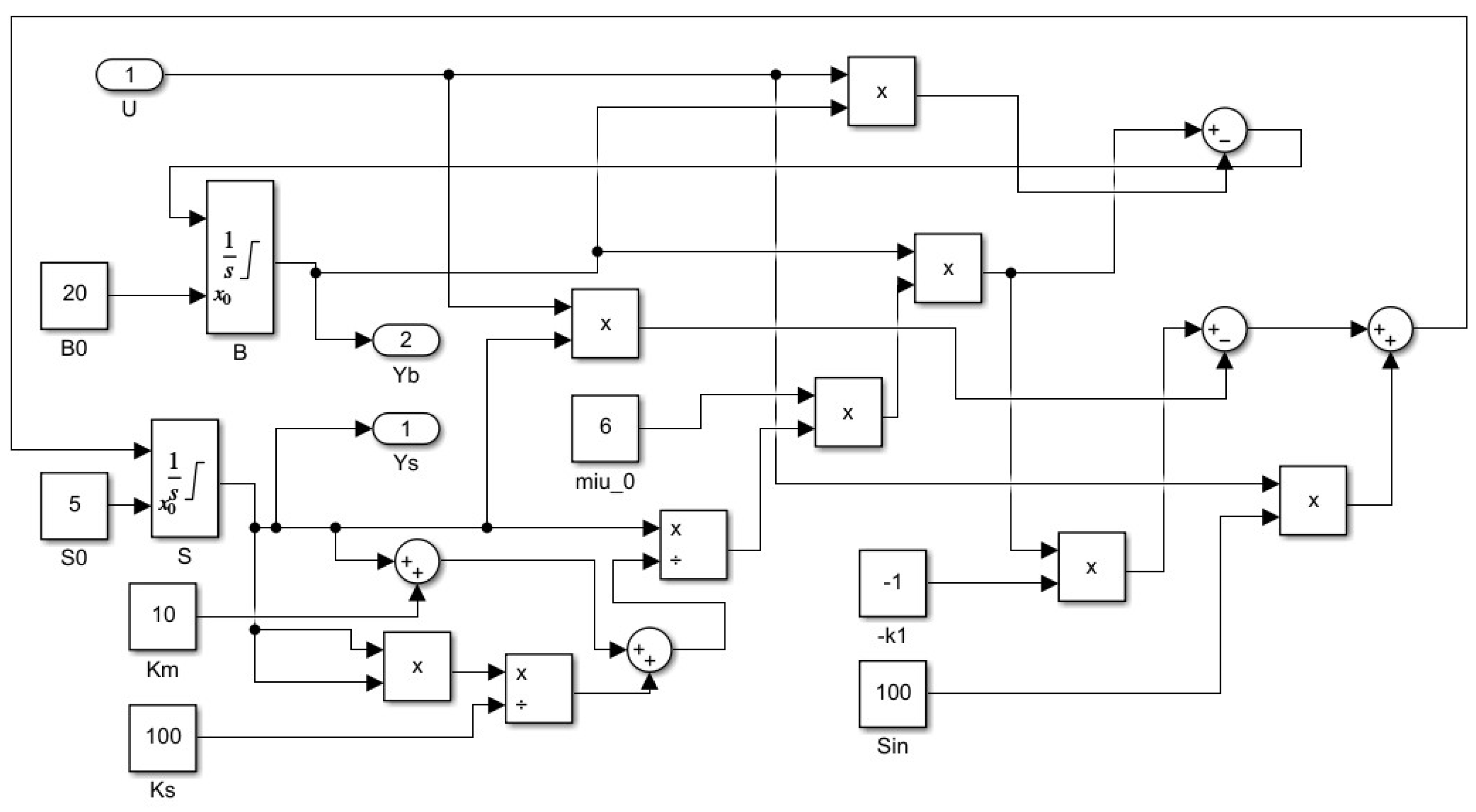
In the following, one presents the model of bacterial growth bioprocess that takes place in a continuous stirred-tank bioreactor. The dynamical model of the process can be expressed in the form of a set of differential equation as follows:

$$\begin{array}{c}\frac{d{\xi }_B}{dt}=\mu \left({\xi }_S\right)\cdot {\xi }_B-D\cdot {\xi }_B\\ \frac{d{\xi }_S}{dt}=-k_1·\mu \left({\xi }_S\right)\cdot {\xi }_B-D\cdot {\xi }_S+F_{in}\end{array},$$

(22)

where ${\xi }_B$ – the biomass concentration, ${\xi }_S$ – the substrate concentration, $F_{in}$ is the input feed rate and $F_{in}=D\cdot S_{in}$ (where $D$ denotes the dilution rate), $S_{in}$ the concentration of influent substrate.

The model can be written in the matrix form:

$$\frac{d}{dt}\left[\begin{array}{c}{\xi }_B\\ {\xi }_S\end{array}\right]=\left[\begin{array}{c}1\\ -k_1\end{array}\right]\cdot \mu \left({\xi }_S\right)\cdot {\xi }_B-D\cdot \left[\begin{array}{c}{\xi }_B\\ {\xi }_S\end{array}\right]+\left[\begin{array}{c}0\\ D\cdot S_{in}\end{array}\right],$$

(23)

and if one denotes

$$\xi =\left[\begin{array}{c}{\xi }_B\\ {\xi }_S\end{array}\right];\mathsf{\Gamma }=\left[\begin{array}{c}1\\ -k_1\end{array}\right];\Phi \left(\xi \right)=\mu \left({\xi }_S\right)\cdot {\xi }_B;F=\left[\begin{array}{c}0\\ D\cdot S_{in}\end{array}\right],$$

(24)

one gets the form (19).

Because it takes into account the inhibitory effect of the substrate at high concentrations, one of the most used models for the specific growth rate is the Haldane model. The Haldane model is described by the following relation:

$$\mu \left({\xi }_S\right)={\mu }_0·\frac{{\xi }_S}{K_M+{\xi }_S+{\xi }_S^2/K_S}$$

(25)

where $K_M$ represents Michaelis-Menten constant, $K_S$ the inhibition constant and ${\mu }_0$ the maximum specific growth rate.

Since

${\left[\frac{\partial \varphi \left(\xi \right)}{\partial {\xi }_B}\right]}_{\xi =\tilde{\xi }}=\mu \left(\widetilde{{\xi }_S}\right)={\mu }_0·\frac{\widetilde{{\xi }_S}}{K_M+\widetilde{{\xi }_S}+\widetilde{{\xi }_S^2}/K_S}$ and

${\left[\frac{\partial \varphi \left(\xi \right)}{\partial {\xi }_S}\right]}_{\xi =\tilde{\xi }}={\left.\frac{d\mu \left({\xi }_S\right)}{d{\xi }_S}\right|}_{\xi =\tilde{\xi }}·{\tilde{\xi }}_B={\mu }_0·{\tilde{\xi }}_B\frac{K_M-{\tilde{\xi }}_S^2/K_S}{{{(K}_M+{\tilde{\xi }}_S+{\tilde{\xi }}_S^2/K_S)}^2}\triangleq \beta$

the linearized matrix has the following form:

$$\mathrm{A}=\left[\begin{array}{cc}\mu \left(\widetilde{{\xi }_S}\right)-\tilde{D}& \beta \\ -k_1\cdot \mu \left(\widetilde{{\xi }_S}\right)& -k_1\cdot \beta -\tilde{D}\end{array}\right],$$

(26)

For the bacterial growth bioprocess, it is important to control the substrate concentration since the too high a value of this concentration leads to the inhibition of biomass growth in the bioreactor [18]. So, one considers ${\xi }_S$ as the controlled variable (output of the system) and the dilution rate D as input. Denoting $y={\xi }_S-\widetilde{{\xi }_S}$ and $u=D-\tilde{D}$, one gets the standard state space representation of a linear system:

$$\left\{\begin{array}{c}\frac{dx}{dt}=A·x+B·u\\ y=C·x\end{array}\right.,$$

(27)

where

$\mathrm{A}=\left[\begin{array}{cc}\mu \left(\widetilde{{\xi }_S}\right)-\tilde{D}& \beta \\ -k_1\cdot \mu \left(\widetilde{{\xi }_S}\right)& -k_1\cdot \beta -\tilde{D}\end{array}\right],B=\left[\begin{array}{c}{-\tilde{\xi }}_B\\ {-{\tilde{\xi }}_S+S}_{in}\end{array}\right],C=\left[01\right]$

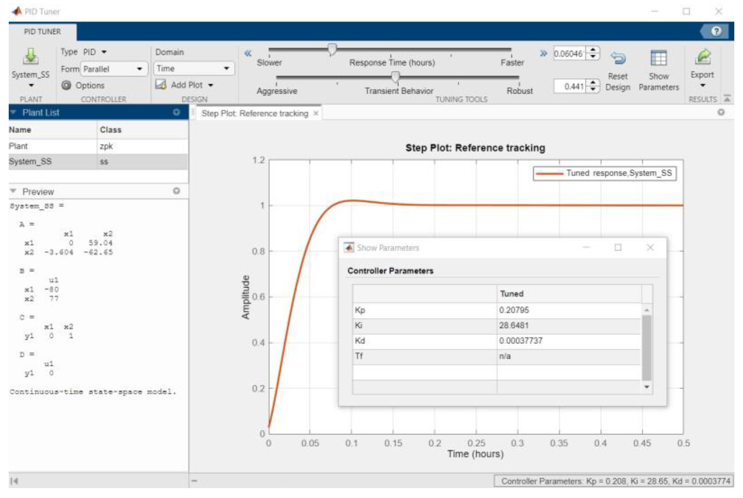
The linearized model (27) can be used to design a PID controller, for example using the PID Tuner app from Matlab [19].

5. Simulation Results

Tuning approaches presented in Section 3 and Section 4 were implemented in Matlab/Simulink environment. The Simulink implementation of bacterial growth bioprocess is presented in Figure 6. The bioprocess parameters used in simulations were the following:

$${\mu }_0=6h^{-1},K_M=\frac{10g}{l},K_S=\frac{100g}{l},k_1=1,S_{in}=\frac{100g}{l}$$

5.1. RL Approach

The Matlab implementation of the PID tuning structure shown in Figure 5 is presented in Figure 7 and is based on RL-TD3 agent implemented in Matlab/Simulink [20].

Observation block has the three elements $\left[P\left(t_n\right)I\left(t_n\right)D\left(t_n\right)\right]$ (see Figure 8), while the Reward block has implemented the formula for the reward. One used a reward function based on LQG criterion:

$$J=\underset{T\to \mathrm{\infty }}{\lim }\left(\frac{1}{T}{\int }_0^T({a·\left(ref-y\right)}^2+\mathrm{b}·u^2(t\left)\right)dt\right),$$

(20)

with $a,b$ two weighting coefficients (see Matlab implementation in Figure 9).

The parameters which are utilized for actor and critic networks of the TD3 agent are presented in Table 2.

The training process is presented in Figure 10.

Figure 9. Training of TD3 neural networks.

Figure 9. Training of TD3 neural networks.

The gains of the PID controller are the absolute weights of the actor representation. After 200 episodes, the following values of the PID controller were obtained:

$K_P=0.62;K_I=3.57;K_D=0.00023$

With gains obtained from the RL agent a step-response simulation was performed. Time evolution of output of the system (substrate concentration) is presented in Figure 10 and command signal and the biomass concentration are presented in Figure 11.

Figure 10. Step response of biotechnological system.

Figure 10. Step response of biotechnological system.

Figure 11. Time evolution of command signal and the biomass concentration.

Figure 11. Time evolution of command signal and the biomass concentration.

5.2. Classical Approach

The nonlinear bioprocess was linearized around the equilibrium point $\tilde{D}=3.6h^{-1},\widetilde{{\xi }_B}=80g/l,\widetilde{{\xi }_S}=23g/l$ . One gets the linear model:

$$\left\{\begin{array}{c}\frac{dx}{dt}=A·x+B·u\\ y=C·x\end{array}\right.$$

with

$$\mathrm{A}=\left[\begin{array}{cc}0& 59.04\\ -3.60& -62.65\end{array}\right]B=\left[\begin{array}{c}-80\\ 77\end{array}\right],C=\left[01\right]$$

The PID controller parameters were tuned using the PID Tuner app from Matlab (see Figure 12). The values of the PID controller are:

$K_P=0.207;K_I=28.64;K_D=0.00037$

Time evolution of output of the system (substrate concentration) is presented in Figure 13 and command signal and the biomass concentration are presented in Figure 14.

From Figure 11 and Figure 14 it can be seen that the control of the substrate is important (too high a value inhibits the concentration of biomass), the main purpose of the regulation system being the increase of biomass production.

The main results and response characteristics are summarized in Table 3.

The response obtained through the classic approach is more aggressive, with a large overshoot and a slightly shorter response time. The response in the case of TD3 based tuning is slower and it has no overshoot.

5. Conclusions

In this paper was proposed the use of learning techniques from the field of artificial intelligence for tuning the parameters of the PID controllers used to control non-linear systems. The proposed method is very useful from a practical point of view because many industrial processes still use PID controllers and their tuning is a particularly important step. Also, many time in practice, empirical tuning methods are used that cannot be used for certain classes of nonlinear systems. The RL-based tuning method is compared with a classical technique that uses the linearization of the nonlinear system around an operating point. In the first case, tuning the controller is done using Twin Delayed Deep Deterministic Policy Gradients (TD3) algorithm which presents a series of advantages compared to other similar RL approaches dedicated to continuous systems. This method is an off-policy Actor-Critic based method and it was chosen as it does not require a system model and works on environments with continuous action and state spaces. In the classical approach, the nonlinear system was linearized around an equilibrium point and then standard tuning methods were used. The presented techniques were applied to the control of a biotechnological system – a bacterial growth process – that take place in a fed-batch bioreactor. The simulations demonstrate the possibility of using machine learning algorithms for tuning the parameters of the PID controllers with the aim of controlling non-linear systems.