Preprint

Article

An Enhanced Particle Swarm Optimization (PSO) Employing Quasi-Random Numbers

Altmetrics

Downloads

Views

Comments

A peer-reviewed article of this preprint also exists.

This version is not peer-reviewed

Submitted:

14 March 2024

Posted:

15 March 2024

You are already at the latest version

Alerts

Abstract

This paper introduces an innovative Particle Swarm Optimization (PSO) Algorithm in-corporating Sobol and Halton Random number samplings. It evaluates the enhanced PSO's performance against conventional PSO employing Monte Carlo Random Number Samplings. The comparison involves assessing the algorithms across nine benchmark problems and the renowned Travelling Salesman Problem (TSP). The re-sults reveal consistent enhancements achieved by the enhanced PSO utilizing Sob-ol/Halton samplings across the benchmark problems. Particularly noteworthy are the substantial improvements demonstrated by the enhanced PSO in solving the Travel-ling Salesman Problem. These findings underscore the efficacy of employing Sobol and Halton random number generation methods in enhancing algorithm efficiency.

Keywords:

Subject: Engineering - Industrial and Manufacturing Engineering

1. Introduction

Particle Swarm Optimization (PSO) is a metaheuristic algorithm for optimization problems. PSO was first introduced in 1995 by James Kennedy and Russell Eberhart [1]. The algorithm is based on the concept of social behavior, where particles (potential solutions) move towards the optimal solution through interactions with other particles in the search space. PSO has been widely used in various fields, including engineering, science, and finance, due to its simplicity, robustness, and efficiency. Despite its success, PSO suffers from several limitations. One of the main limitations is its slow convergence rate, which can be attributed to the premature convergence [2] of the particles towards local optima. This issue can be addressed by introducing efficient improvement techniques in PSO. Several enhancement ideas have been proposed in the past to improve the convergence rate of the PSO algorithm, and they are listed below. Firstly, the Inertia weight technique was suggested by Russell Eberhart and Ying Shi [3]. The inertia weight technique is a well-known approach for enhancing the convergence speed of PSO. The inertia weight is used to control the movement of particles in the search space. The idea is to maintain a balance between exploration and exploitation of the search space. The inertia weight is updated at each iteration based on a predefined formula, which controls the speed and direction of particle movement. Various formulas have been proposed for updating the inertia weight, such as linear, nonlinear, and adaptive. The choice of the inertia weight formula depends on the optimization problem and the PSO parameters. Second, the concept of a mutation operator was proposed [4]. A mutation operator is a powerful tool for enhancing the diversity of the PSO population. The mutation operator randomly modifies the position of a particle to generate a new solution in the search space. This operation can prevent premature convergence by introducing new solutions that may lead to better solutions. The mutation operator can be applied at different stages of the PSO algorithm, such as before or after the velocity update. Third, the Opposition-based Learning technique was suggested [5]. Opposition-based learning (OBL) is a technique that uses the opposite of the current best solution to generate new solutions. The idea behind OBL is that the opposite of the best solution may represent a good direction for exploration in the search space. OBL can improve the diversity and convergence speed of PSO by generating new solutions that are different from those of the current population. Fourth, hybridization with other metaheuristics has been proposed [6]. Hybridization with other metaheuristics is a common approach for improving the efficiency of PSO. The idea is to combine the strengths of different metaheuristics to overcome their weaknesses. For example, PSO can be combined with genetic algorithms (GA), simulated annealing (SA), or ant colony optimization (ACO). The hybridization approach can enhance the exploration and exploitation capabilities of PSO, leading to better solutions in less time. Fifth, Dynamic parameter Tuning was presented [6]. The PSO parameters, such as the swarm size, maximum velocity, and acceleration coefficients, significantly impact the algorithm's performance. Dynamic parameter tuning is a technique that adjusts the PSO parameters based on the search history during the optimization process. The idea is to adapt the PSO parameters to the problem characteristics and the search progress to improve the convergence speed and solution quality. In conclusion, efficient improvement techniques in PSO can enhance the algorithm's convergence speed and solution quality. The approaches discussed in this paper [6], including the inertia weight technique, mutation operator, opposition-based learning, hybridization with other metaheuristics, and dynamic parameter tuning, can be used individually or in combination to address the limitations of PSO. Tareq M. Shami and a team [7] of researchers conducted a comprehensive survey on PSO. The survey discusses techniques such as varying the inertia weight and hybridizations, which are discussed above. The survey also states that the ability of PSO to be hybridized with other optimization algorithms has contributed to its popularity. Another technique described in the survey which is velocity clamping [7], a technique introduced by Eberhart and Kennedy. Velocity clamping is setting bounds for the values of the velocities of the particles in all the dimensions. Another approach to improving the efficiency of the PSO algorithm discussed in this paper [7] is varying the controlling parameters, such as using the varying inertia weight technique in which inertia weight changes throughout the optimization process, or acceleration coefficient techniques in which the two constant controlling parameters for PSO other than the inertia, are chosen in different ways to yield optimal solutions while evading premature convergence. Many other approaches have been discussed both in the survey, and elsewhere. The choice of approach depends on the problem characteristics and the available computational resources. However, most of these approaches can provide problem-dependent solution methods. In this paper, we proposed a new approach to replace the random numbers used for this method with quasi-random numbers [8,9,10] like Halton and Sobol by maintaining the k-dimensional uniformity of these quasi-random numbers. This not only provides a generalized approach to any kind of optimization problem, but this method can be used in conjunction with the earlier enhancement techniques like the inertia weight technique, mutation operator, opposition-based learning, hybridization with other metaheuristics, and dynamic parameter tuning. In this research, two enhanced versions of PSO (one using Sobol random numbers and the other using Halton random numbers) were proposed with the intention of speeding up the convergence of the standard PSO algorithm. To test the efficiency improvement of the two proposed enhancements of the standard PSO algorithm, the number of iterations taken to achieve the optimum of the well-known cigar, ellipsoid, and paraboloid functions, along with the number of iterations taken to obtain an optimal path for the famous Travelling Salesman Problem (TSP) were noted. Following this, improvement in terms of the optimum of the objective function and the number of iterations needed to reach the global optimum were calculated for both the PSO enhanced with Sobol random number samplings and the PSO enhanced with Halton random number samplings, with respect to the standard PSO which uses Monte Carlo random number samplings. All the results for each benchmark function and TSP unanimously show efficiency improvement due to the use of Sobol and Halton Sequences. Additionally, we noted that the more decision variables an optimization problem has, the improvement due to Sobol and Halton sequences increases. In conclusion, both the enhancements of the standard PSO presented in this research, one utilizing Sobol random numbers and the other utilizing Halton random numbers, consistently show efficiency improvement and a better optimum, meaning that they successfully have increased the speed of convergence of the standard PSO algorithm.

2. Materials and Methods

2.1. Particle Swarm Optimization

There are countless examples of swarms in the real world, ranging from flocking birds to hunting wolves. When searching for nourishment, the individuals of these swarms, called particles to understand PSO, begin random exploration and then start gravitating towards the findings of other swarm individuals. While following signs of nourishment and searching randomly in space, through knowledge of their discoveries and discoveries of the swarm, these particles move towards their objective. Similarly, in the PSO algorithm, proposed decision variable sets gravitate towards the optimal findings of each other, themselves, and the whole swarm together to achieve the globally optimal set of decision variables, yielding the optimal function value. The sets of decision variables are called position vectors. They are updated by vectors called velocity vectors (based on the physics principle that change in position is proportional to the velocity), by randomness, and by attraction towards their personal best sets of decision variables and the unanimous global best set of decision variables found by the whole swarm. Through gradual movement towards optimal findings of the swarm, the global optimum of the function is achieved. The following are the steps of the PSO algorithm.

Initialize Parameters:

Define the population size (number of particles), $N p$
Define the number of decision variables (dimension), $D$
Define the maximum number of iterations, $T$ .
Define the inertia weight, $ω$
Define acceleration constants: cognitive and social, $c_{1}, c_{2}$ .
Initialize the position and velocity of each particle randomly within the search space.

The initially proposed set of solutions is grouped together to form the population matrix which is written as

[\begin{matrix} x_{0}^{00} & \dots & x_{0}^{0 (D - 1)} \\ ⋮ & ⋱ & ⋮ \\ x_{0}^{(N p - 1) 0} & \dots & x_{0}^{(N p - 1) (D - 1)} \end{matrix}]

Each row in this matrix represents a potential decision variable vector that is intended to optimize the objective function. Each element in a row is the position with respect to a particular dimension of the particle that corresponds with that row. The subscript for each element is 0, as these values are the initial values in the matrix (0th iteration).

The velocity matrix can be represented as:

[\begin{matrix} v_{0}^{00} & \dots & v_{0}^{0 (D - 1)} \\ ⋮ & ⋱ & ⋮ \\ v_{0}^{(N p - 1) 0} & \dots & v_{0}^{(N p - 1) (D - 1)} \end{matrix}]

This represents the velocity of each particle in all the dimensions. The position matrix is changed by the velocity matrix, and that is inspired by the physics concept that displacement is proportional to velocity. The superscript

j

is the index of the dimension.

Set the best-known position for each particle n, $P_{n}^{i j}$ to its initial position.

$P^{j} = x^{0 j}$

Evaluate Fitness:

Evaluate the fitness (objective function value) for each particle based on its current position.

Update the personal best position for each particle $G_{n}^{j}$ if its current fitness is better than its previous best fitness.

Update Global Best:

g.: Determine the particle with the best fitness among all particles in the swarm, $P_{n}^{*}$ .
h.: Update the global best position with the position of the particle with the best fitness, $G_{n}^{*}$ .
i.: Update Velocities and Positions:

For each particle, update its velocity and position based on the following formulae:

The velocity of each particle at iteration

n

is updated according to the Equation,

v_{n + 1}^{i j} = ω * v_{n}^{i j} + c_{1} * r_{1} * (P_{n}^{j} - X_{n}^{i j}) + c_{2} * r_{2} * ({G_{n}}^{j} - X_{n}^{i j})

(1)

where

r_{1}

and

r_{2}

are random numbers. So, we have 2 random numbers per variable.

And the corresponding position is updated according to the Equation,

{x_{n + 1}}^{i j} = {x_{n}}^{i j} + v_{n + 1}^{i j}

(2)

Check Stopping Criteria:

j.: If the maximum number of iterations is reached or a satisfactory solution is found, stop the algorithm.
k.: Otherwise, go back to step 2 and repeat the process.

Output:

Return the global best position as the solution to the optimization problem..

2.2. Quasi-Random Sequence Enhancements

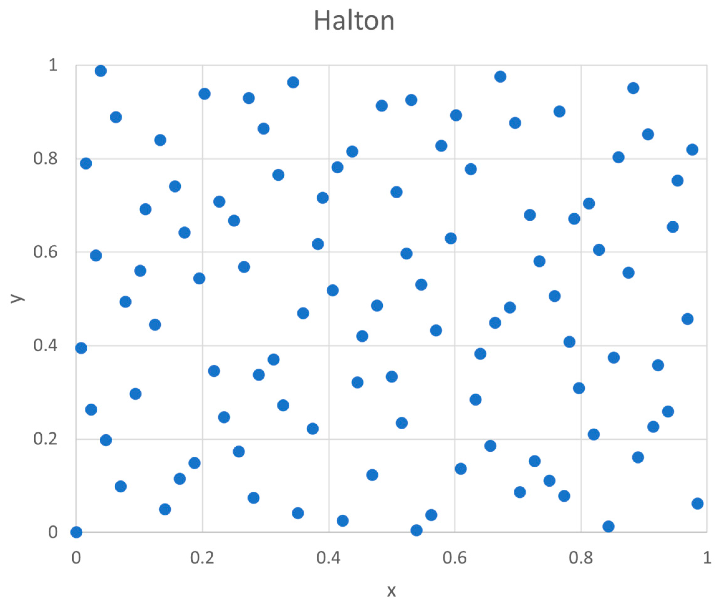
In this work, we hypothesize that the success of PSO depends on the choice of appropriate random samples. At each iteration of PSO, two random numbers are generated for each decision variable, as shown in Equation (1). These random numbers are computer-generated random numbers and are called pseudorandom numbers or Monte Carlo random numbers. A sequence of random numbers must have two essential properties: uniformity, i.e., they are equally probable everywhere, and independence, i.e., the current value of a random variable has no relation with the previous values. Figure 1 shows the two random variables generated using computer (Monte Carlo or pseudo random numbers) with samples equal to 100. As can be seen in the figure, for uniformity, the points should be equally distributed; that is not the case here. We need more samples to cover the points equally in that 2-dimensional space. This means more iterations of the algorithm. To circumvent this problem and to increase the efficiency of PSO, we are presenting a construct based on quasi-random numbers. Some well-known quasi-random sequences are Halton, Hammersley, Sobol, Faure, Korobov, and Neiderreiter [8,9,10]. The choice of an appropriate quasi-Monte Carlo sequence is a function of discrepancy. Discrepancy is a quantitative measure of the deviation of the sequence from the uniform distribution. Therefore, it is desirable to choose a low discrepancy sequence. The Halton, SOBOL, and Hammersley are some examples of low-discrepancy sequences. Here, we are working with the two sequences, Halton and SOBOL, described below.

2.3. Halton Sequence Points

The design of Halton points is given below. Any integer n can be written in radix-R notation (R is an integer) as follows:

n \equiv n_{m} n_{m - 1} ... n_{2} n_{1} n_{0}

(3)

n = n_{0} + n_{1} R + n_{2} R^{2} + ... + n_{m} R^{m}

(4)

where

m = [\log_{R} n] = [\ln n / \ln R]

(the square brackets denote the integral part). A unique fraction between 0 and 1 called the inverse radix number can be constructed by reversing the order of the digits of n around the decimal point as follows:

φ_{R} (n) = n_{0} n_{1} n_{2} ... n_{m} = n_{0} R^{- 1} + n_{1} R^{- 2} + ... + n_{m} R^{- m - 1}

(5)

The Halton points on a k-dimensional cube are given by the following sequence:

\vec{z_{k}} (n) = (φ_{R_{1}} (n), φ_{R_{2}} (n), . . ., φ_{R_{k - 1}} (n)), n = 1,2, . . . ., N + 1

(6)

where R1, R2,…, Rk-1 are the first k-1 prime numbers. The Halton points are

\vec{x_{k}} (n) = 1 - \vec{z_{k}} (n)

Figure 2 shows 2-dimensional Halton points (100 samples) showing better uniformity than Figure 1.

2.4. SOBOL Sequence Points

Like many other quasi-random sequences, the SOBOL sequence starts from the Van der Corput sequence in base 2. To generate the Vander Corput sequence, consider the k-th point in the Sobol sequence; this integer k can be written as a linear combination of a nonnegative power of base 2 as follows.

k = a_{0} (k) + 2 a_{1} (k) + 2^{2} a_{2} (k) + \dots + 2^{r} a_{r} (k)

(7)

where r is a large number.

Then, the k-th element in the Sobol sequence is given by

x^{k} = {1 / 2 y}_{1} (k) + 1 / 2^{2} y_{2} (k) + \dots + 1 / 2^{r} y_{r} (k)

(8)

where the coefficients

y_{i} (k)

can be obtained using the following expression

\{\begin{matrix} y_{1} (k) \\ y_{2} (k) \\ \dots \\ y_{r} (k) \end{matrix}\} = V \{\begin{matrix} a_{0} (k) \\ a_{1} (k) \\ \dots \\ a_{r - 1} (k) \end{matrix}\} \mod 2

(9)

where V is the generation matrix whose elements are 0 or 1. V is an identity matrix for Vander Corput sequence.

The operation in equation 9 can be represented as

a_{0} (k) V_{1} \oplus a_{1} (k) V_{2} \oplus a_{2} (k) v_{3} \dots a_{r - 1} (k) V_{r}

where

V_{i}

is an element of V and

\oplus d e n o t e s b i n a r y a d d i t i o n

The calculation of generation matrix V involves primitive polynomial A primitive polynomial of degree d, all the coefficients A1 to Ad-1 are either 1 or 0 are given below.

P = X^{d} + A_{1} X^{d - 1} + \dots + A_{d - 1} X + 1

(10)

Direction vectors

M_{i}

are generated by a recursive equation given below for i > d, and the initial direction vectors, i.e., for i < d, are generated by selecting an odd integer between 0 &

2^{d}

M_{i} = 2^{1} A_{1} M_{i - 1} \oplus 2^{2} A_{2} M_{i - 2} \oplus \dots \dots \dots \oplus 2^{d - 1} A_{d - 1} M_{i - d + 1} \oplus 2^{d} M_{i - d} \oplus M_{i - d}

(11)

Then, the generation matrix elements can be generated as given below.

V_{i}^{j} = \frac{M_{i}}{2^{i}}

(12)

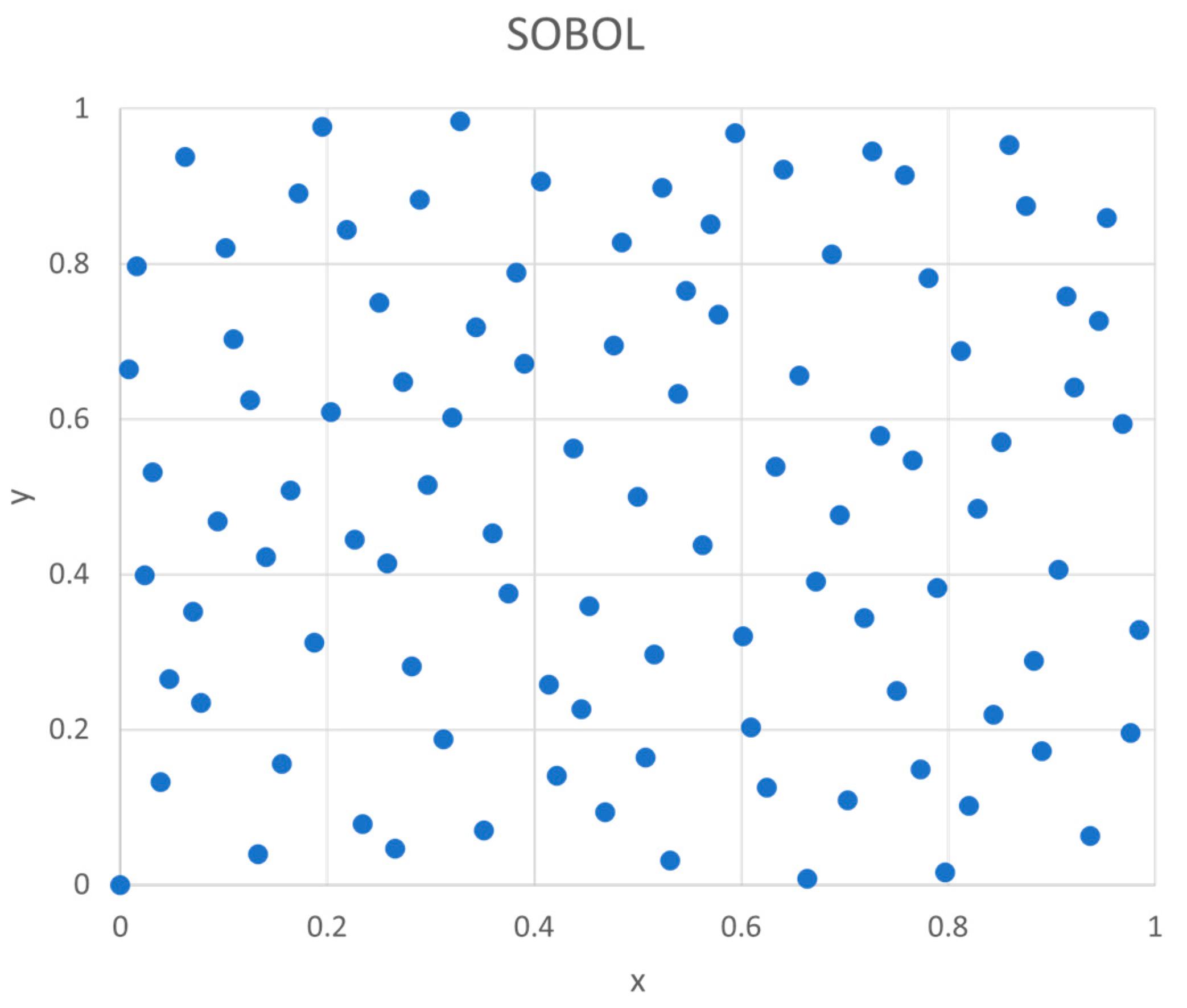
Thus, SOBOL sequence can be generated by generating the V matrix and the Van der Corput sequence in base 2

.

Figure 3 shows that SOBOL points show better uniformity than pseudo random numbers from computer (Figure 1).

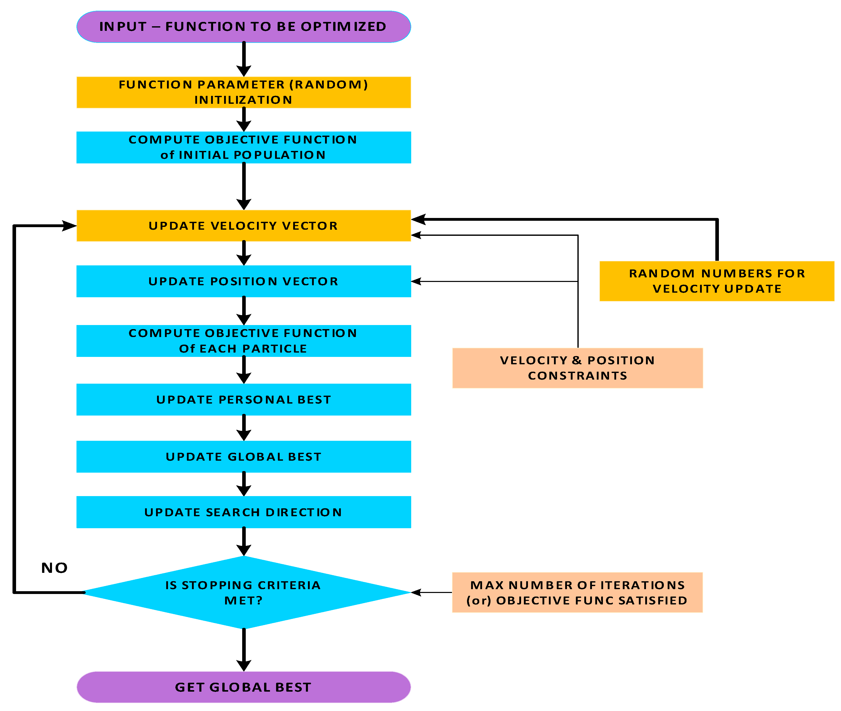
We show where the random numbers are used in PSO with traditional PSO in Figure 4 and Enhanced PSO with Halton or SOBOL in Figure 5. However, to maintain k-dimensional uniformity, the Halton and SOBOL points cannot be generated one at a time; they must be generated together with the whole sample (for all iterations).

It should be noted that all other efficiency enhancements proposed in the literature can be directly applicable to our new algorithms as we are only changing the random numbers.

3. Results

3.1. Test Cases

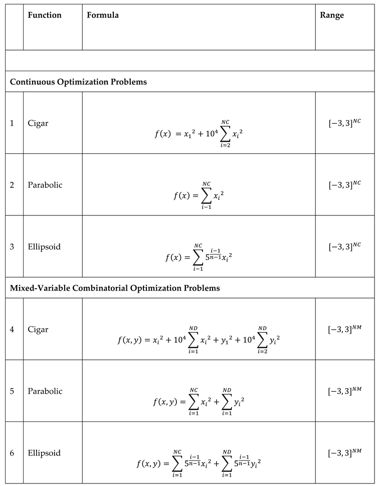
To test the efficiency improvements of the enhanced PSO suggested in this paper, both mixed and continuous versions of three well-known benchmark functions, namely the Cigar, Ellipsoid, and Paraboloid functions, along with the famous Travelling Salesman problem, are taken as test cases (Table 1). Three algorithms consisting of one PSO code with no enhancement (using Monte Carlo random number samplings), a second PSO code that uses Sobol random number samplings, and a third PSO code that uses Halton random numbers are each run for 5, 10, 15, and 20 decision variables, to optimize both the mixed and continuous versions of the three benchmark functions and to solve the TSP problem. The number of iterations taken to achieve an optimum is recorded for all three algorithms to reach the global optimum.

3.2. Traveling Salesman Problem Optimization Procedure

The traveling salesman problem [12] is a discrete combinatorial optimization problem. The locations of many cities are given, and an optimal order in which the cities are traversed is to be calculated. A position vector is the suggested order of cities. The velocity vector is a sequence of two-element tuples in which each tuple consists of two indices of elements to be swapped to make the path more optimal. For example, if there are five cities labeled with indices {1, 2, 3, 4, 5}, the population matrix could consist of different suggested orders in which they are to be traversed, such as {2, 4, 3, 5, 1} and {5, 4, 3, 1, 2}. The velocity vector for the first suggested order of cities could be {(1, 2), (3, 2), (4, 5)} while for the second it could be {(5, 1)}. In this case, the first element would be swapped with the second, the third with the second after that, and the fifth with the fourth after that, in the first suggested sequence of cities. For the second, the fifth and first elements are to be swapped.

ω

α

, and

β

are pre-determined constants used in this algorithm. A random number is generated for each swap in the previous velocity vector. For each random number that is less than

ω

, the corresponding swap is included in the new velocity vector. Similarly, this process is done for the second term and the third term with

α

and Beta instead of

ω

. These three random numbers are generated together to maintain the k-dimensional uniformity of the quasi-random number sequence when Halton or SOBOL is used. Through the usage of this swapping method, the optimal order in which the cities must be visited is to be attained.

For

i - t h p a r t i c l e a t i t e r a t i o n i n d e x n, t o u p d a t e v e l o c i t y w e h a v e :

v_{n + 1}^{i} = {ω * v_{n}^{i}} ⨁ \{α * (P_{n}^{i} - X_{n}^{i})\} ⨁ \{β * (G_{n}^{j} - X_{n}^{i})\}

H e n c e, v_{n + 1}^{i} i s a s e t o f s w a p s .

Here, the ⊕ is the merging operator, which merges sequences of swaps into a new swap sequence.

α < 1, β < 1 a n d ω < 1

For

i - t h p a r t i c l e a t i t e r a t i o n i n d e x n

, apply the new updated velocity

v_{n + 1}^{i}

to the current position

X_{n}^{i}, (

which is a set of Node sequence or Node list in TSP) and obtain the updated position

X_{n + 1}^{i} .

X_{n + 1}^{i} = X_{n}^{i} \overset{A p p l y S w a p s}{\leftarrow} v_{n + 1}^{i}

{ω * v}_{n}

means is if

v_{n}

is a vector of L elements to begin with, then L random numbers are generated and for each random number that is less than

ω,

the corresponding swap in

v_{n}

is used.

(P_{n}^{i} - X_{n}^{i}) i s

a swap sequence to move from

X_{n}^{i}

P_{n}^{i}

. For example if

P_{n}^{i}

is {3, 4, 5, 2, 1} and

X_{n}^{i} i s \{5, 3, 4, 1, 2\}, t h e s e t o f s w a p s n e e d e d t o m o v e f r o m X_{n}^{i}

P_{n}^{i}

is {(1, 3), (3, 2), (4, 5)} (Assuming that indices start from 1).

α * (P_{n}^{i} - X_{n}^{i}) i s

a set of swaps that are selected from the swap sequence vector

(P_{n}^{i} - X_{n}^{i})

of length N based on the N random numbers generated which are less than

α .

During initialization, for each particle

i

X_{0}^{i} a r e

set to a random selection of cities whose IDs are the city node index. If there are N cities to be visited, then

X_{0}^{i}

is a vector of length N.

The following are tables comparing the results produced by Monte Carlo Random Number Sampling with Sobol Random Number Sampling and Halton Random Number Sampling.

3.3. Sobol vs. Monte Carlo Random Numbers

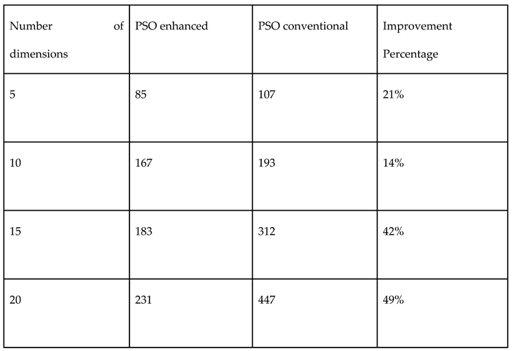
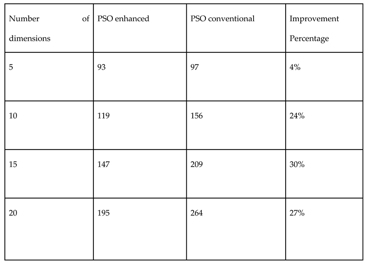
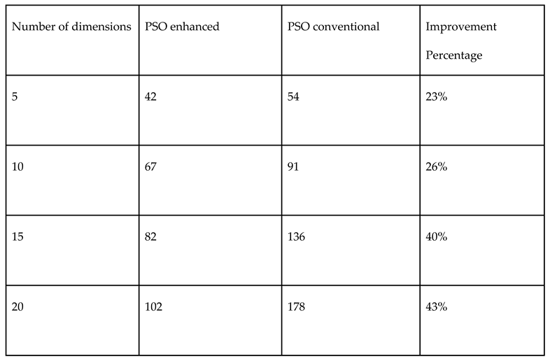
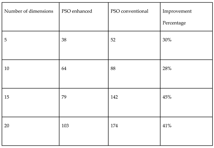
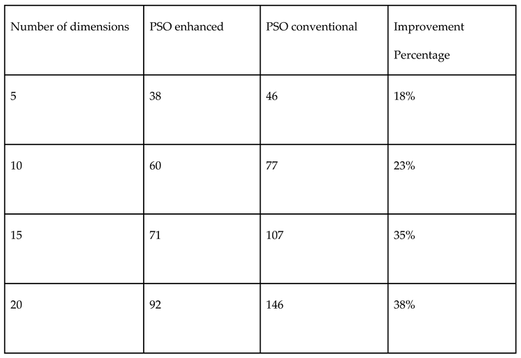
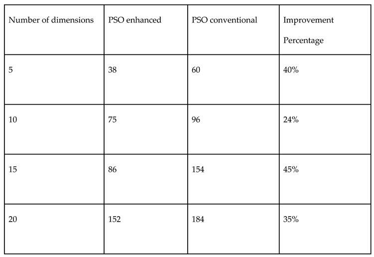
We compare the performance of using SOBOL versus Pseudorandom numbers for the three functions (continuous and mixed variable form) in Table 2, Table 3, Table 4, Table 5 and Table 6.

Table 2. Comparison of performances of both Monte Carlo and Sobol random number samplings in PSO for continuous variable Cigar function.

Table 3. Comparison of performances of both Monte Carlo and Sobol random number samplings in PSO for mixed variable Cigar function.

Table 4. Comparison of performances of both Monte Carlo and Sobol random number samplings in PSO for continuous variable Paraboloid function.

Table 5. Comparison of performances of both Monte Carlo and Sobol random number samplings in PSO for mixed variable Paraboloid function.

Table 5. Comparison of performances of both Monte Carlo and Sobol random number samplings in PSO for continuous variable Ellipsoid function.

Table 6. Comparison of performances of both Monte Carlo and Sobol random number samplings in PSO for mixed variable Ellipsoid function.

3.4. Halton vs. Monte Carlo

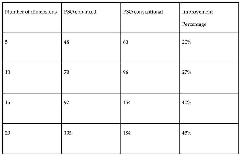
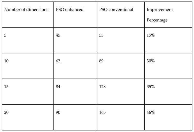
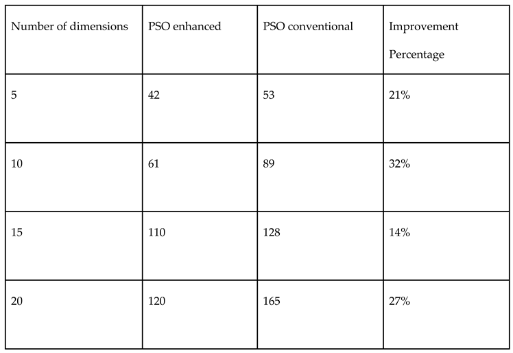
The results of Halton-based enhanced PSO are presented in Table 7, Table 8, Table 9, Table 10, Table 11 and Table 12.

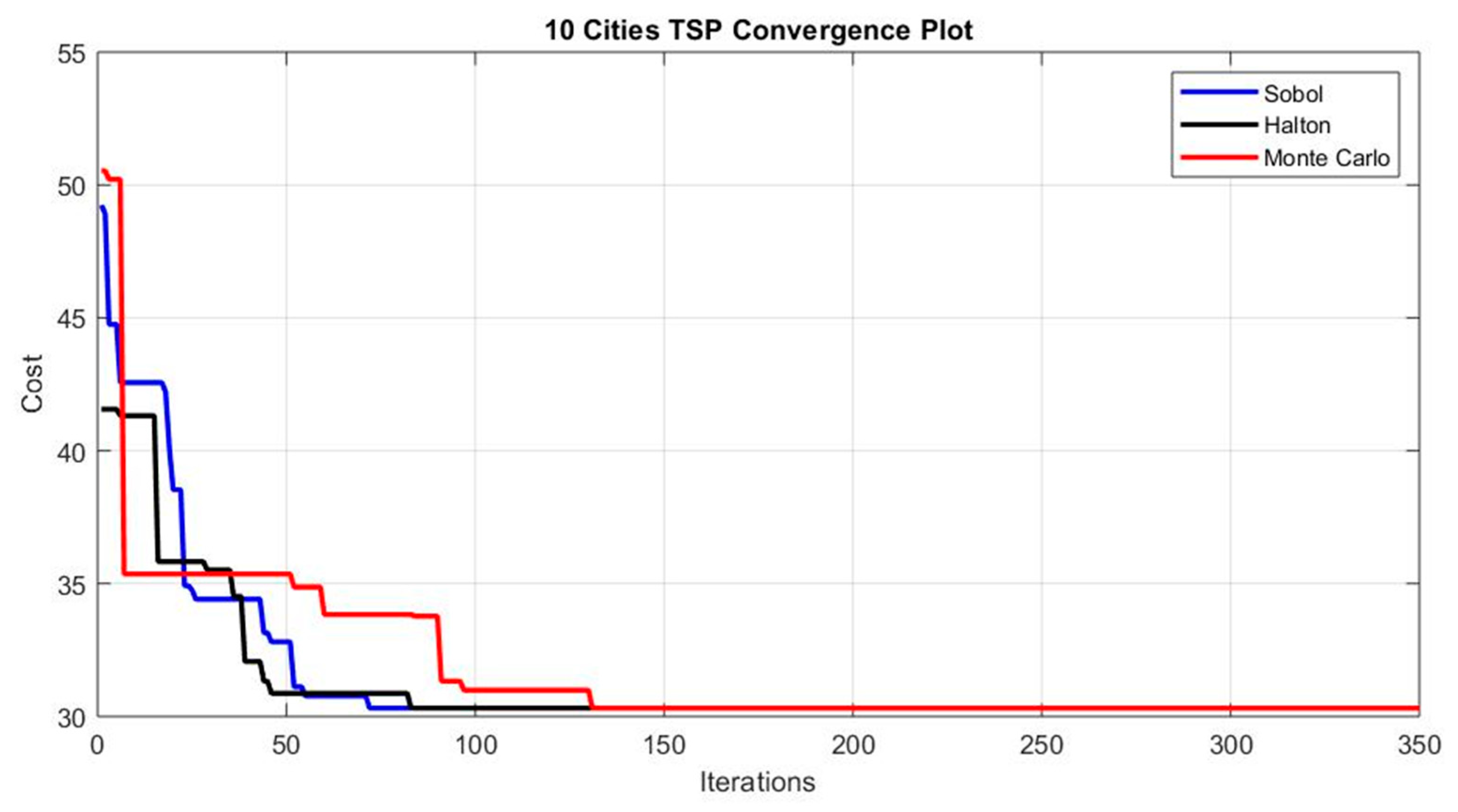
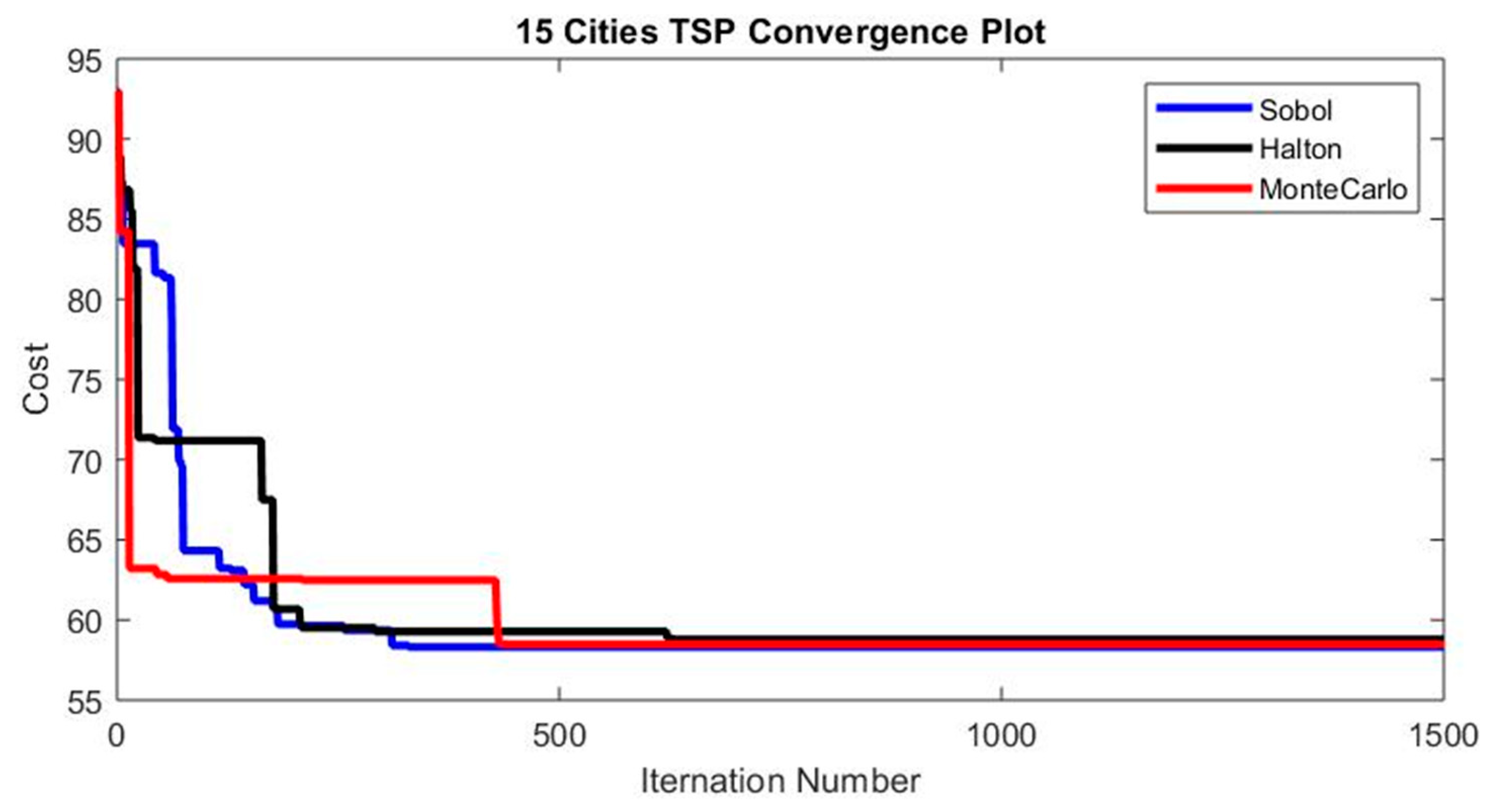
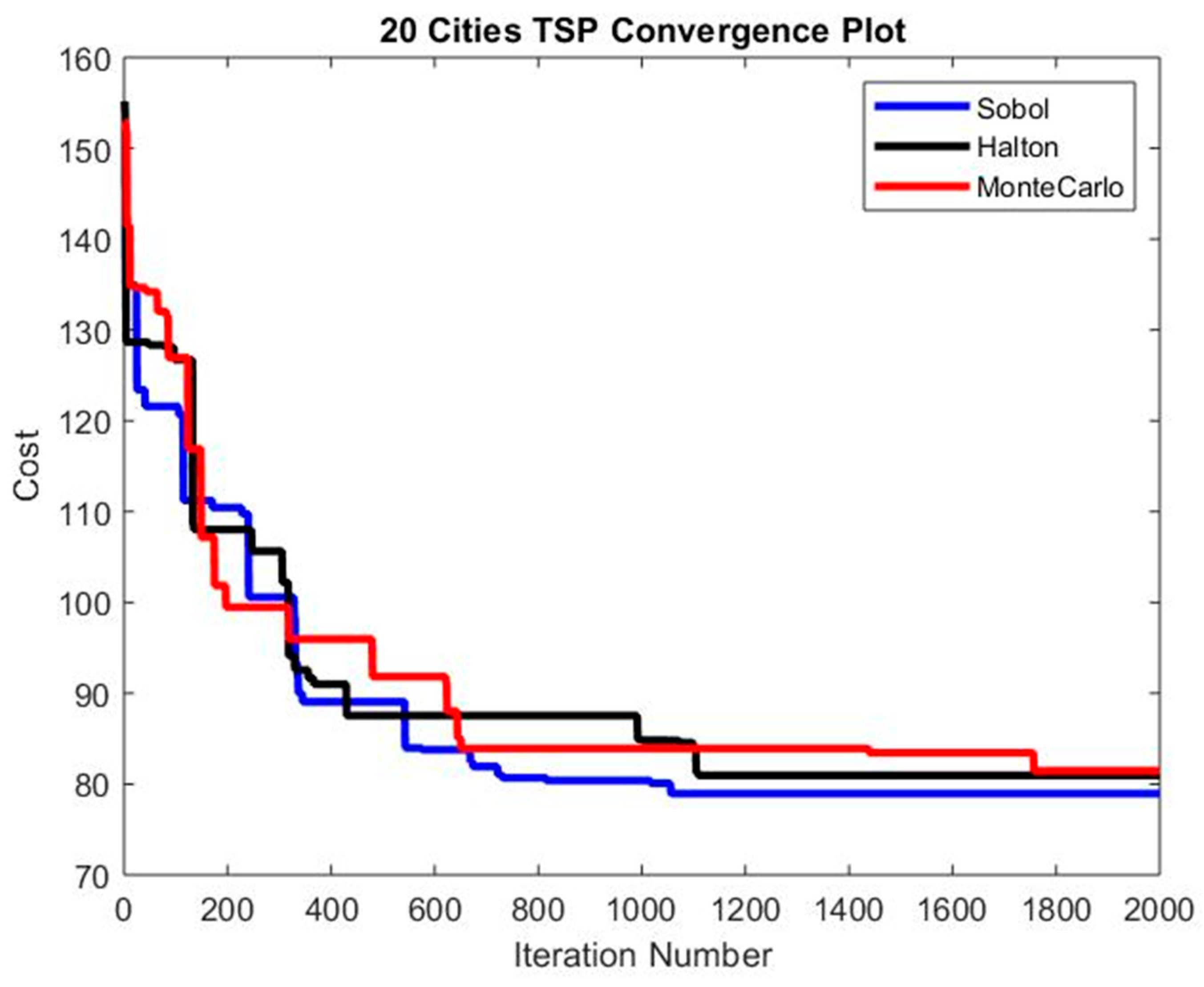
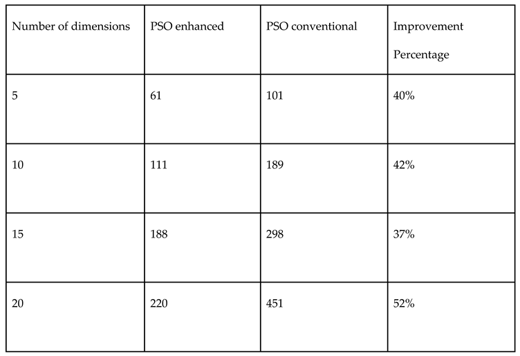
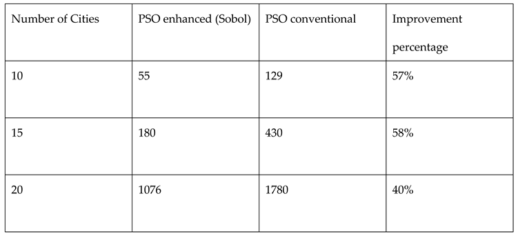
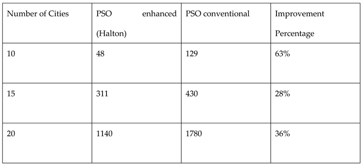
It can be seen from the above tables (Tables 2 to 12) that the quasi-random sequences-based enhanced PSO performs superior to a conventional random number-based PSO for both continuous and mixed variable problems. The enhancement increases generally with a higher number of variables specifically for continuous variable problems. SOBOL serves better for mixed variable functions than Halton, but Halton shows better convergence than SOBOL when considering continuous variables. Table 13 and Table 14 provide the TSP comparison. TSP is a completely discrete problem, and SOBOL performs better, as can be seen from Figure 6, Figure 7 and Figure 8, and Table 13 and Table 14.

4. Discussion

We have augmented the PSO algorithm by integrating Sobol and Halton random number samplings to achieve superior results. Our rationale behind this enhancement is rooted in Sobol and Halton random numbers, quasi-random numbers. These numbers are generated in such a manner that they are uniformly distributed across multidimensional space, thus mitigating clustering or bias in particle movement. Consequently, this facilitates more extensive exploration, thereby increasing the likelihood of avoiding local optima and accelerating the discovery of the global optimum, as a more significant portion of the space can be explored when biases or clusters are circumvented. The outcomes indicate that the enhancement applied to the standard PSO through the utilization of quasi-random numbers has consistently improved the number of iterations required for the algorithm to produce the optimal function value across all three benchmark functions. The efficiency gains for continuous functions are more pronounced than those for mixed variable functions.

Additionally, including more decision variables in the problem correlates with more significant improvements in general. As evident from the data, the application of Sobol or Halton sequences to the standard PSO algorithm demonstrates efficiency improvements, suggesting the potential benefits of these sequences to researchers in various optimization fields. Notably, this technique is algorithm-agnostic, as indicated in the introduction, and can thus be employed with other optimization algorithms such as the Genetic Algorithm, Ant Colony Optimization (ACO) algorithm, and other established optimization algorithms.

5. Conclusions

Particle Swarm Optimization harnesses swarm behavior effectively for function optimization but is often hampered by slow convergence. We have consistently improved efficiency through two distinct enhancements to the Particle Swarm Optimization algorithm. We proposed using quasi-random number sequences to update decision variable values and their rates of change in each iteration to enhance the PSO algorithm. Since quasi-random number sequences do not alter the fundamental algorithm, this concept can be integrated into modified versions of the PSO algorithm suggested previously, as discussed in the introduction. To evaluate whether quasi-random number sequences in PSO yield efficiency improvements, we tested them using continuous and mixed variable Cigar, Ellipsoid, and Paraboloid functions, along with an example of the Traveling Salesman problem. The results demonstrate that both sequences of quasi-random numbers used to enhance the standard PSO have improved efficiency.

Author Contributions

Conceptualization, UD. methodology, UD.; software, SK.; validation, SK.,; formal analysis, SK and UD.; investigation, SK and UD; resources, UD.; data curation, SK.; writing—original draft preparation, SK.; writing—review and editing, UD.; visualization, SK and UD.; supervision, UD.; project administration, UD. All authors have read and agreed to the published version of the manuscript.

Funding

This research received no external funding.

Data Availability Statement

Data can be obtained from authors.

Conflicts of Interest

The authors declare no conflicts of interest.

References

T.M. Shami, A. A. T.M. Shami, A. A. El-Saleh, M. Alswaitti, Q. Al-Tashi, M. A. Summakieh and S. Mirjalili, “Particle Swarm Optimization: A Comprehensive Survey,” in IEEE Access, vol. 10, pp. 100131-10061, 2022. [CrossRef]
J. Kennedy and R. Eberhart, "Particle swarm optimization," Proceedings of ICNN'95 - International Conference on Neural Networks, Perth, WA, Australia, 1995, pp. 1942-1948 vol.4. [CrossRef]
J. C. Bansal, P. K. J. C. Bansal, P. K. Singh, M. Saraswat, A. Verma, S. S. Jadon and A. Abraham, "Inertia Weight strategies in Particle Swarm Optimization," 2011 Third World Congress on Nature and Biologically Inspired Computing, Salamanca, Spain, 2011, pp. 633-640. [CrossRef]
Ning Li, Yuan-Qing Qin, De-Bao Sun and Tong Zou, "Particle swarm optimization with mutation operator," Proceedings of 2004 International Conference on Machine Learning and Cybernetics (IEEE Cat. No.04EX826), Shanghai, China, 2004, pp. 2251-2256 vol.4. [CrossRef]
Z. Zhou, F. Z. Zhou, F. Li, J. H. Abawajy and C. Gao, "Improved PSO Algorithm Integrated With Opposition-Based Learning and Tentative Perception in Networked Data Centers," in IEEE Access, vol. 8, pp. 55872-55880, 2020. [CrossRef]
B. Mandal, P. K. B. Mandal, P. K. Roy and S. Mandal, "Hybridization of Particle Swarm Optimization with Biogeography-Based Optimization for Reactive Power and Voltage Control," 2014 Fourth International Conference of Emerging Applications of Information Technology, Kolkata, India, 2014, pp. 34-39. [CrossRef]
Y. Cai and S. X. Yang, "An improved PSO-based approach with dynamic parameter tuning for cooperative target searching of multi-robots," 2014 World Automation Congress (WAC), Waikoloa, HI, USA, 2014, pp. 616-621. [CrossRef]
Morokoff, William J., and Russel E. Caflisch. “Quasi-Random Sequences and Their Discrepancies.”. SIAM Journal on Scientific Computing 1994, 15, 1251–1279. [CrossRef]
Niederreiter, Harald. 1992. Random Number Generation and Quasi-Monte Carlo Methods. CBMS-NSF Regional Conference Series in Applied Mathematics 63. Philadelphia, Pa: Society for Industrial and Applied Mathematics.
Sobol, I.M. Uniformly distributed sequences with an additional uniform property. USSR Journal of Computational Mathematics and Mathematical Physics (English translation) 1976, 16, 1332–1337. [Google Scholar] [CrossRef]
Diwekar UM, Gebreslassie BH (2016) Efficient Ant Colony Optimization (EACO) Algorithm for Deterministic Optimization. Int J Swarm Intel Evol Comput 5: 131. [CrossRef]
Sarman, K. Hadia, Arjun H. Joshi, Chaitalee K. Patel, Yogesh P. Kosta, “Solving City Routing Issue with Particle Swarm Optimization”. International Journal of Computer Applications 2012, 47. [Google Scholar]

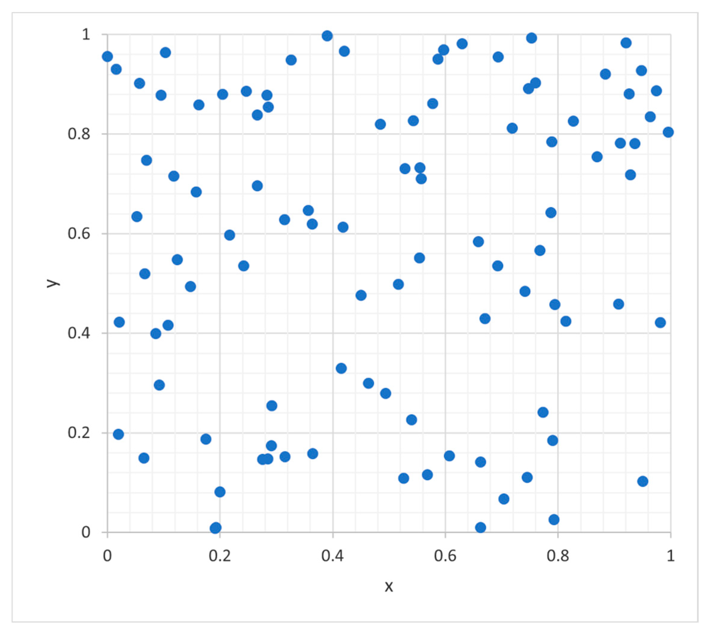
Figure 1. 2-dimensional pseudorandom numbers (100 points).

Figure 2. Dimensional Halton Points (100).

Figure 3. 2-dimensional SOBOL points (100).

Figure 4. Traditional PSO Flowchart.

Figure 5. Enhanced PSO Flowchart.

Figure 6. TSP with 10 Cities – Convergence Plot.

Figure 7. TSP with 15 Cities – Convergence Plot.

Figure 8. TSP with 20 Cities – Convergence Plot.

Table 1. Test Cases for Algorithm Testing [11].

Table 7. Comparison of performances of both Monte Carlo and (scrambled) Halton random number samplings in PSO for Continuous variable Cigar function.

Table 8. Comparison of performances of both Monte Carlo and (scrambled) Halton random number samplings in PSO for Mixed variable Cigar function.

Table 9. Comparison of performances of both Monte Carlo and Halton random number samplings in PSO for continuous variable Paraboloid function.

Table 10. Comparison of performances of both Monte Carlo and Halton random number samplings in PSO for mixed variable Paraboloid function.

Table 11. Comparison of performances of both Monte Carlo and Halton random number samplings in PSO for continuous variable Ellipsoid function.

Table 12. Comparison of performances of both Monte Carlo and Halton random number samplings in PSO for mixed variable Ellipsoid function.

Table 13. Comparison of performances for Monte Carlo and Sobol random number samplings in PSO for TSP.

Table 14. Comparison of performances for Monte Carlo and Halton random number samplings in PSO for TSP.

Disclaimer/Publisher’s Note: The statements, opinions and data contained in all publications are solely those of the individual author(s) and contributor(s) and not of MDPI and/or the editor(s). MDPI and/or the editor(s) disclaim responsibility for any injury to people or property resulting from any ideas, methods, instructions or products referred to in the content.

© 2024 by the authors. Licensee MDPI, Basel, Switzerland. This article is an open access article distributed under the terms and conditions of the Creative Commons Attribution (CC BY) license (http://creativecommons.org/licenses/by/4.0/).

Copyright: This open access article is published under a Creative Commons CC BY 4.0 license, which permit the free download, distribution, and reuse, provided that the author and preprint are cited in any reuse.

MDPI Initiatives

Important Links

Choose an area of interest and we will send you notifications of new preprints at your preferred frequency.

Disclaimer

An Enhanced Particle Swarm Optimization (PSO) Employing Quasi-Random Numbers

Abstract

1. Introduction

2. Materials and Methods

2.1. Particle Swarm Optimization

2.2. Quasi-Random Sequence Enhancements

2.3. Halton Sequence Points

2.4. SOBOL Sequence Points

3. Results

3.1. Test Cases

3.2. Traveling Salesman Problem Optimization Procedure

3.3. Sobol vs. Monte Carlo Random Numbers

3.4. Halton vs. Monte Carlo

4. Discussion

5. Conclusions

Author Contributions

Funding

Data Availability Statement

Conflicts of Interest

References

MDPI Initiatives

Important Links

Subscribe