1. Introduction
Numerous research results show that long wavelength N.D. Kondratiev (K-waves) play an important role in forecasting economic crises and cycles [
1,
2,
3,
4,
5,
6,
7,
8,
9,
10,
11,
12,
13,
14,
15,
16,
17,
18,
19,
20,
21,
22,
23,
24,
25,
26,
27,
28,
29,
30,
31,
32,
33,
34]. K-waves can be described using dynamic (oscillatory) systems, which mainly characterize nonlinear oscillatory processes [
11,
14,
18,
27]. Such processes are studied to describe the chaotic and regular dynamics of nonlinear oscillatory systems. In world practice, identifying chaotic regimes, for example, in clinical medicine or in the study of turbulence in the atmosphere, is one of the main tasks. Regular modes of nonlinear oscillations are of particular interest when studying economic cycles and crises, various chemical reactions, biological systems, etc. [
35,
36]. Nonlinear oscillatory processes within the framework of the K-wave theory can also have heredity (memory) effects, which can be described from a mathematical point of view using derivatives of fractional orders [
37,
38,
39,
40,
41].
In the review work of Tarasov V.E. [
42] provides 260 literature sources on the application of fractional derivatives to various economic processes. This article contains a brief overview of the stages in the history of the application of fractional calculus in modern mathematical economics and economic theory. The first stage of the application of heredity in economics is associated with the works published in 1966 and 1980 by Clive W. J. Granger [
43,
44], who received the Nobel Prize in Economics in 2003. Further, the history of the application of fractional calculus in economics can be divided into the following five stages of development (approaches): ARFIMA [
43,
44]; fractional Brownian motion [
45]; econophysics [
46,
47]; deterministic chaos [
48]; mathematical economics [
49,
50]. The modern stage (mathematical economics) is intended to include new economic concepts and concepts into modern economic theory that allow us to take into account the presence of memory in economic processes. Further in the review article some comments are given on possible further directions for the development of fractional mathematical economics.
In this article, within the framework of mathematical economics, we will study K-waves using a generalization of the classical mathematical model of S.V. Dubovsky, proposed in the article [
14] for the case of memory effects. Note that K-waves are well described in monographs [
15,
16,
17,
20,
21,
22,
24]. However, an analysis of the literature on the research topic showed that the application of fractional calculus to the dynamic system of S.V. Dubovsky has not yet been carried out to describe K-waves. In addition, even the classical dynamical system of S.V. Dubovsky without taking into account heredity (with integer derivatives), proposed in the article [
14], did not take into account the influx of external investments and new technologies, as well as the rate of accumulation as a function of capital productivity. Therefore, the proposed mathematical models with derivatives of fractional constant and variable orders in the sense of Gerasimov-Caputo are completely new objects of study in this article.
The main objective of the study is to establish the existence of closed phase trajectories in the proposed fractional mathematical models. Next, in the presence of closed trajectories, using computer modeling, study how the values of various parameters of the model and their various functional dependencies influence the shape of these cycles, as well as study cycles for stability. Of course, along the way, other dynamic regimes arise that also deserve research.
The research plan in the article is structured as follows. The first section provides an overview of the current state of research on the theory of K-waves, revealing some problems that have not been studied within the framework of the classical model of S.V. Dubovsky and which are solved in this article. The second section examines the classical model of S.V. Dubovsky: the basic equations of the model are derived, and two modifications of the model are given - taking into account the rate of accumulation depending on capital productivity and external inflow of investments and new technologies. It is shown using Bendixson’s theorem that the proposed model can have a closed phase trajectory. Oscillograms and phase trajectories were constructed using the Adams-Bashforth-Moulton numerical algorithm and an interpretation of the research results was given. The third section provides a generalization of the classical model of S.V. Dubovsky in the case of taking into account constant heredity: the definition of the fractional derivative in the sense of Gerasimov-Caputo is given, the Cauchy problem is posed, which is studied by the Adams-Bashforth-Moulton numerical method, the order of convergence of the method is studied using the Runge rule, oscillograms and phase trajectories are constructed for various values of the model parameters and an interpretation of the research results is given. The fourth section provides a generalization of the fractional model of S.V. Dubovsky in the case of taking into account variable heredity: the definition of a derivative of a fractional variable order of the Gerasimov-Caputo type is introduced, the Cauchy problem is posed, which is studied using the Adams-Bashforth-Moulton numerical method, the order of convergence of the method is studied using the Runge rule, oscillograms and phase trajectories are constructed for various values of the model parameters, an interpretation of the research results is given. The fifth section provides conclusions based on the results of the study, and also indicates their possible further development.
2. Classical mathematical model of S.V. Dubovsky and some modifications for describing K-waves
In this section, the classical mathematical model of S.V. was studied. Dubovsky to describe long waves N.D. Kondratiev (K-waves). This model describes the dynamics of free fluctuations in the efficiency of new technologies and the efficiency of capital productivity. From the point of view of mathematics, it is a system of nonlinear ordinary differential equations of the first order (Cauchy problem).
The purpose of the research is to visualize the results of the solution using numerical modeling, taking into account the modification of the mathematical model of S.V. Dubovsky, which consists in taking into account the dependence of the accumulation rate on capital productivity and external inflow of investments and new technological solutions.
2.1. Derivation of the basic equations of the classical mathematical model by S.V. Dubovsky
Derivation of the basic equations of the classical mathematical model by S.V. Dubovsky
where
is gross domestic product,
is capital,
is the average technological level of the economy,
n is the accumulation rate,
is the capital depreciation rate,
l is the employment growth rate,
is the latest technological level for newly introduced fixed production assets.
On the right side of equation (
1), in order to simplify the model, all types of income from production and/or other capital (working capital, banking, etc.) not used for investment are omitted. Equation (
1) includes an indicator of quantitative measurement of the results of scientific and technological progress according to Harrod, which increases labor productivity.
Differential equation (
2), more interesting from the point of view of revealing the fundamentals of the production function, is the standard equation for the dynamics of the overall production function.
A more detailed derivation of equation (
3) to describe the dynamics of the average technological level (the standard equation used in economics) is presented in a number of scientific works by S.V. Dubovsky [
14,
25].
S.V. Dubovsky based on the model of N.D. Kondratiev and standard equations reflecting economic dynamics, in particular, equations for the rate of employment growth and the rate of depreciation of production assets, the latter depending on the rate of renewal of the latter, expressed the general interaction and interdependence in the form of the following formulas:
here the parameters with zero indices take their constant value at the initial time.
Relations (
4) are transformed into an equation for new variables: capital productivity efficiency:
; efficiency of new technologies:
.
Based on formula (
5) S.V. Dubovsky derived a differential equation to describe the dynamics of the efficiency of new technologies, taking into account the assumption that the growth of the latest technological level is proportional to the latest technological level and its relative efficiency, as well as financial indicators - the rate of accumulation and return on assets.
The above assumption of S.V. Dubovsky formally wrote this as the following equation:
where
a and
b are constant parameters.
Equation (
6) divided by
and taking into account relation (
4) allowed S.V. Dubovsky write down the differential equation for the variable
in the form of equation (
4):
As a result, S.V. Dubovsky managed to reduce the basic model (
1)-
3 to a system of two nonlinear differential equations (
5) and (
7) with respect to two variables — the efficiency of new technologies
and capital productivity
. Here, the first term, as a rule, correlates with economic profit, and the second with the depreciation of production assets and the costs of capital owners.
Remark 1. It is necessary to emphasize that system (5) and (7) has an equilibrium stationary solution: , which agrees well with real statistics.
Introduction of new variables — variations relative to the point
in the form:
, S.V. Dubovsky obtained from equations (
5) and (
7) linear differential equations in variations:
Having multiplied equations (
8) by suitable coefficients, S.V. Dubovsky obtained the following relation (first integral):
Equation (
9) obtained by S.V. Dubovsky describes a family of ellipses for different values of the derivative of the constant
C.
2.2. Statement of the problem, solution method and its properties
Based on equations (
5) and (
7) in article [
14] S.V. Dubovsky proposed the following Cauchy problem
where
are functions of the efficiency of new technologies and capital productivity,
— process time,
— simulation time,
— accumulation rate,
— constant coefficient, which is determined from statistics,
and
are constant values that correspond to the rest point of the system,
a and
b are given constants that determine the initial conditions,
.
Definition 1. We will call the system of nonlinear differential equations (10), which represents the Cauchy problem, the Classical Mathematical Model of S.V. Dubovsky (CMMD).
Remark 2. Note that the classical mathematical model of S.V. Dubovsky (10) describes free nonlinear fluctuations in the efficiency of new technologies and capital productivity.
Let us show that the dynamical system (
10) can have closed phase trajectories. To do this, we introduce the following definition.
Definition 2. A simply connected region Ω is a region in which all closed paths are homotopic to zero, i.e., they can be continuously contracted to a point. This means that the region does not contain holes or self-intersections.
Let
and
— right sides (
10), which are continuous functions,
is a vector field defined in the simply connected domain
. Then the following theorem is true.
Theorem 1. (Bendixson’s theorem [51]) If the divergence of the vector field f does not change sign and is nonzero throughout the entire region Ω, then the phase trajectories of the autonomous system of differential equations do not have closed trajectories that lie entirely in Ω.
Theorem 2. An autonomous system of differential equations (10) can have closed phase trajectories.
Proof. Using Theorem 1, we can show that the divergence of the vector field
f changes its sign and is not identically zero in a simply connected domain.
Then
From the economic meaning of the problem parameters (
,
) we can conclude that the change in the sign of the function (
11) in a simply connected domain
can occur. Indeed, if you choose
Then the divergence of the vector field
f will change its sign in the simply connected region. If condition (
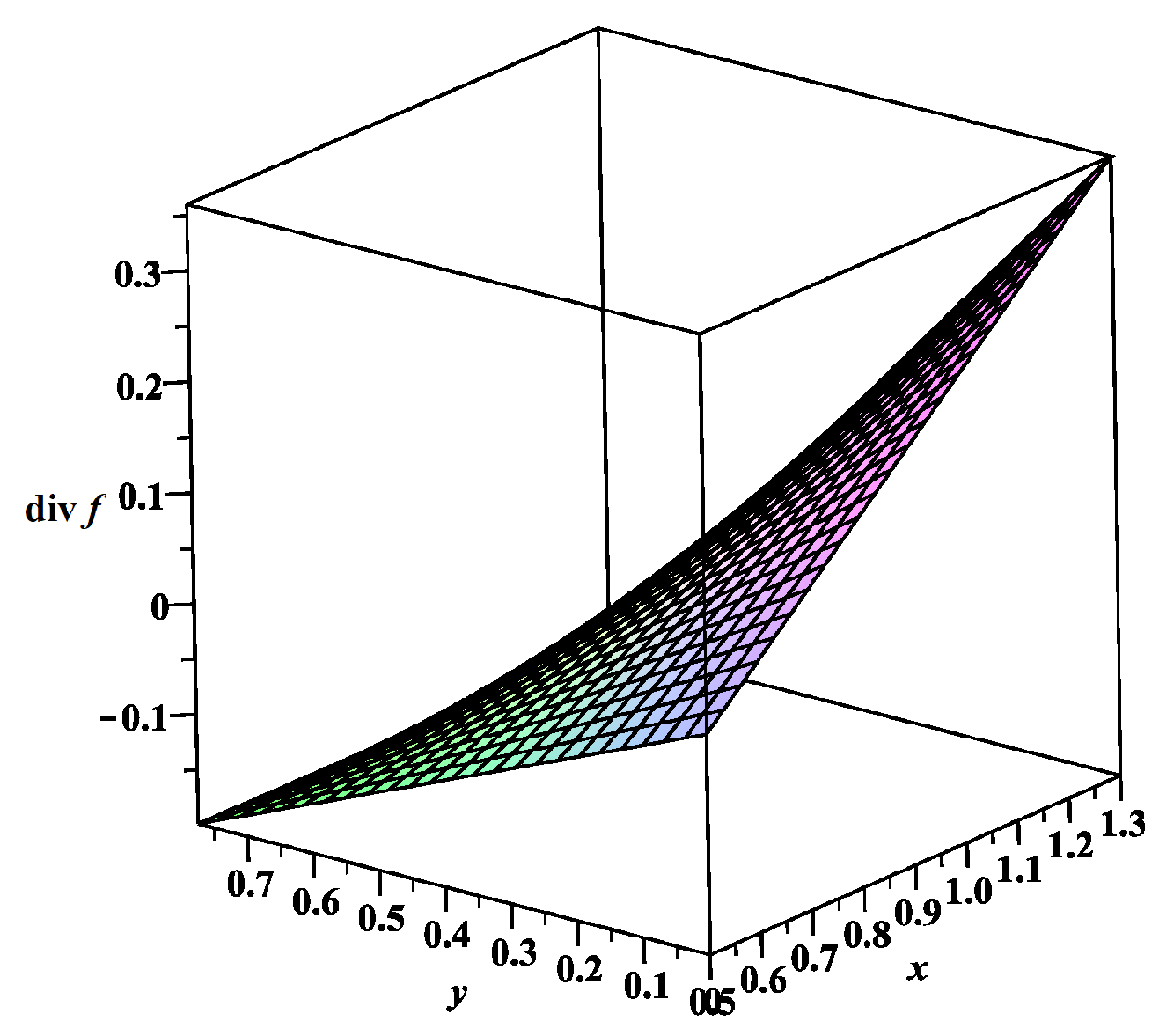
12) is violated, then the divergence retains its sign. Using the visualization tools of the Maple computer mathematics environment, we will construct an example of a simply connected region in which the sign changes for the parameter values are performed (
Figure 1):
.
Based on the above, we can conclude that system (
10) may have closed phase trajectories. □
The theorem indicates that the classical mathematical model of S.V. Dubovsky (
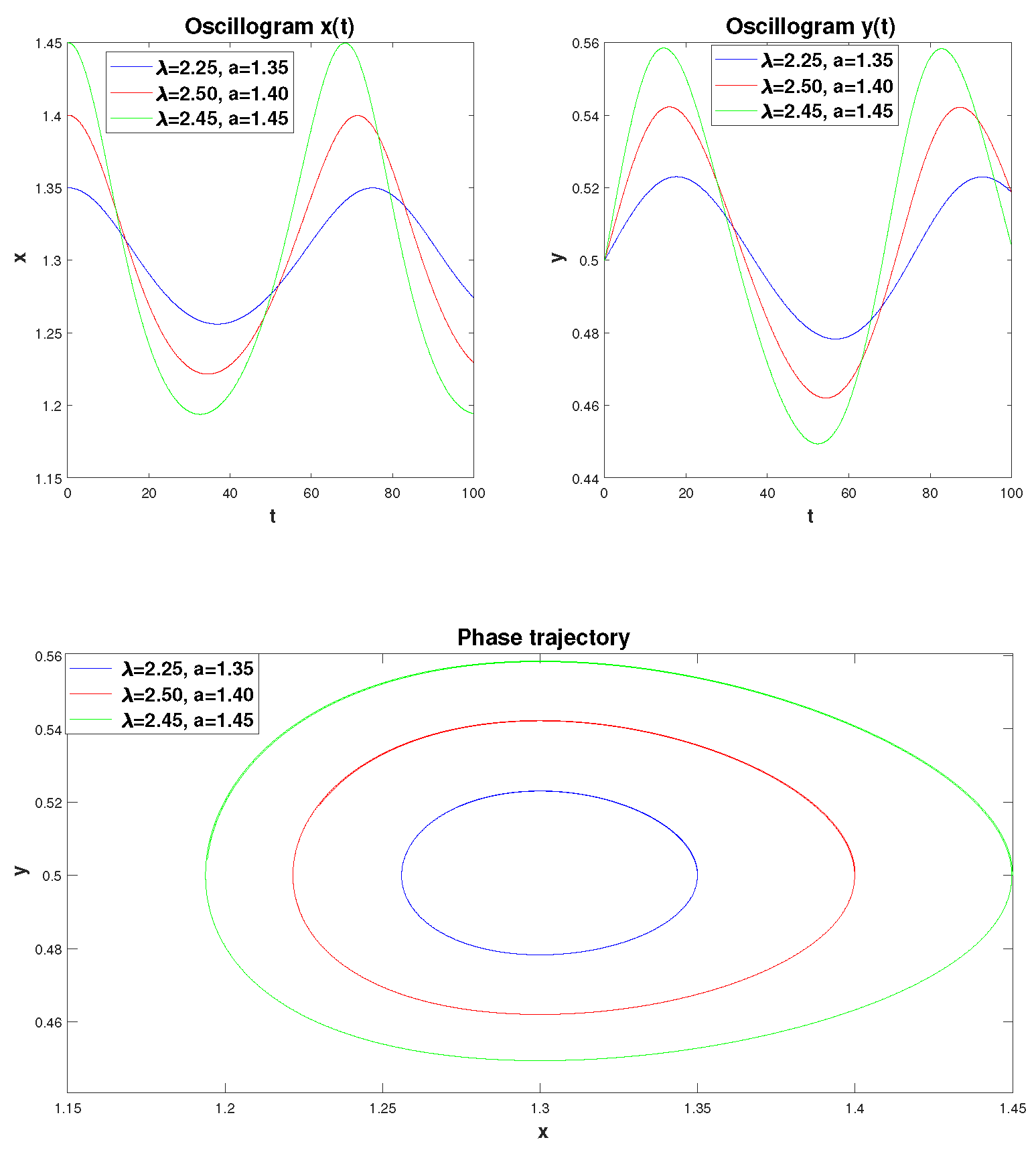
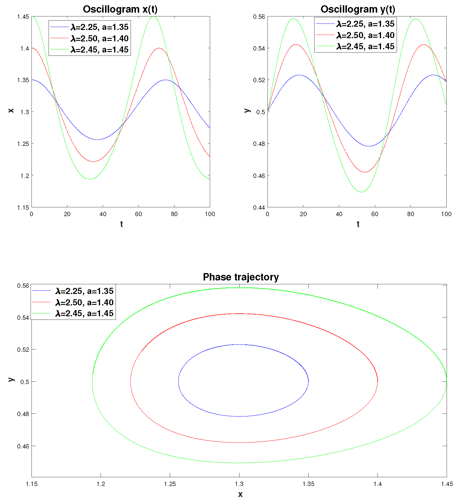
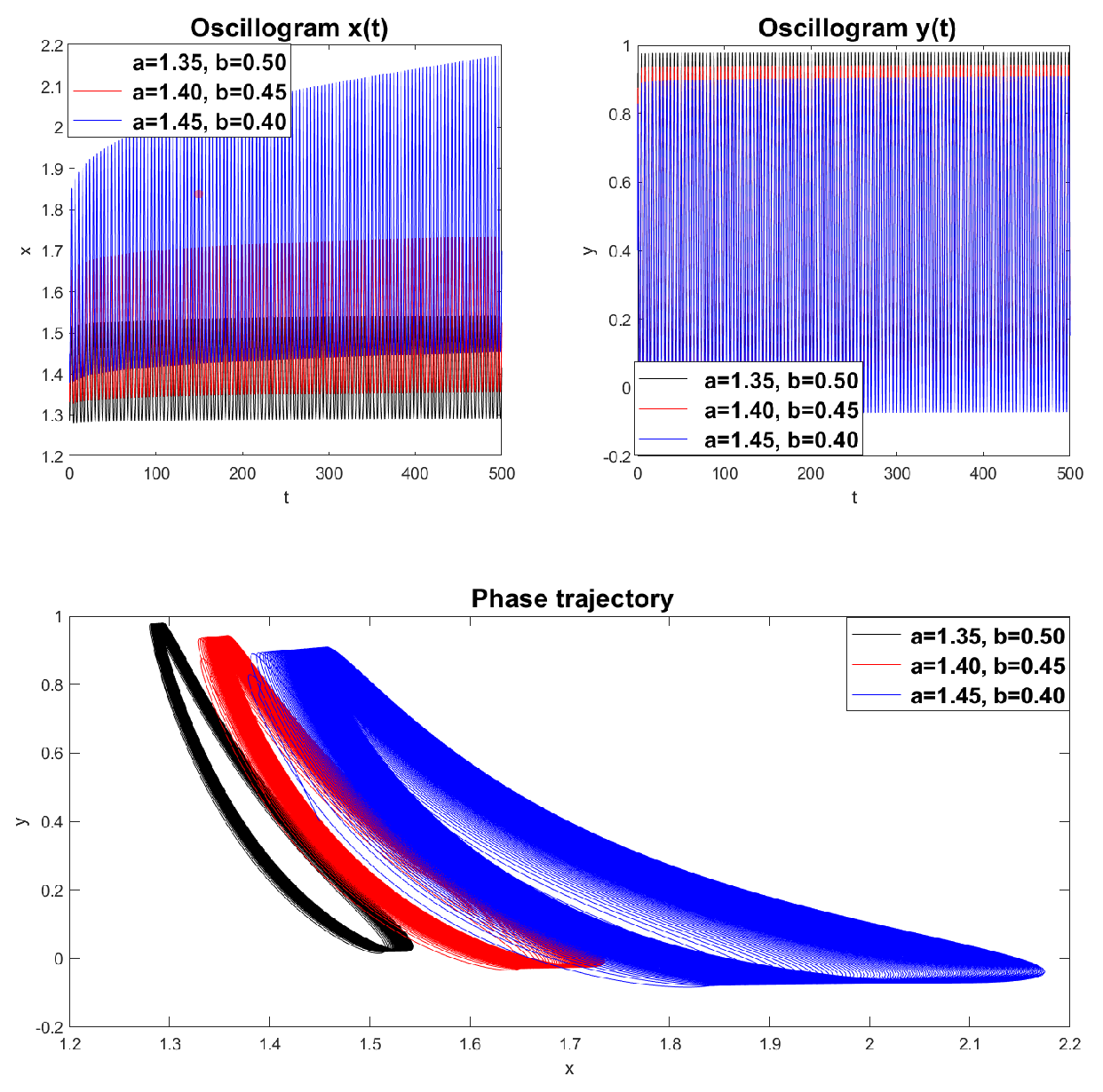
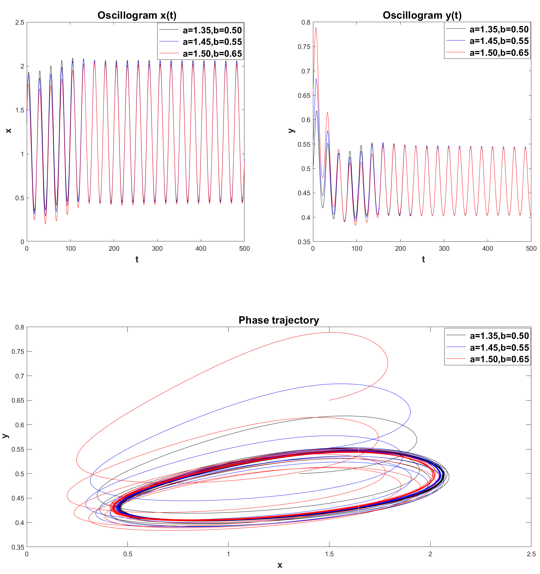
10) can be suitable for studying cyclical regimes that can arise in the theory of economic cycles and crises. Let’s construct oscillograms and phase trajectories for the classical model of S.V. Dubovsky for different values of the initial conditions
a and parameter
(
Figure 2). For this purpose, we will use the one-step Adams-Bashforth-Moulton method (ABM) of the 2nd order of convergence (trapezoidal rule) [
52], which was implemented in the MATLAB computer algebra system.
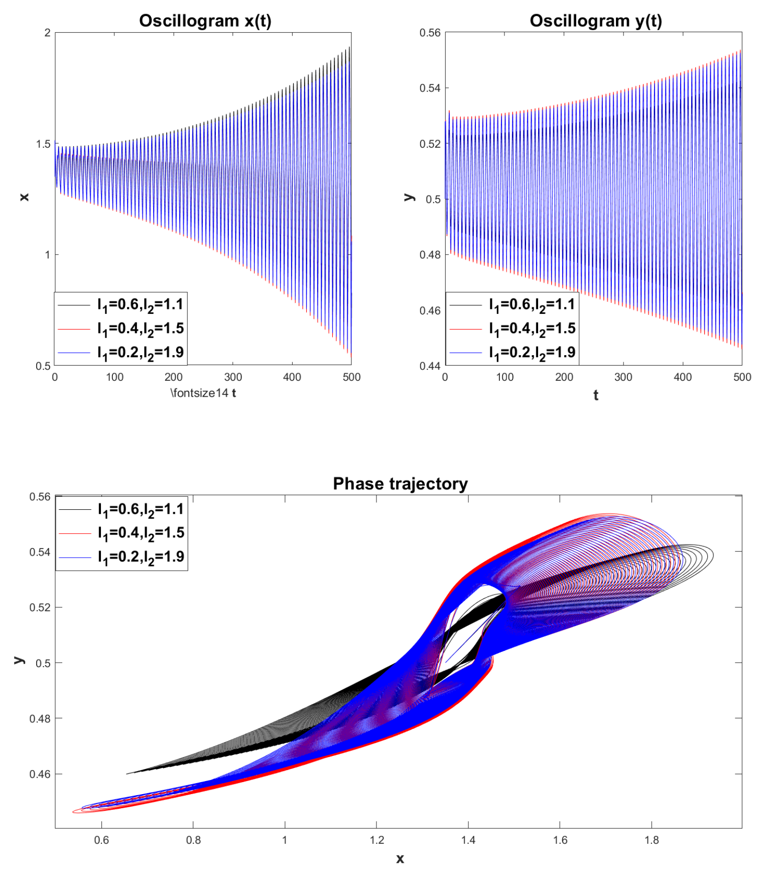
From
Figure 2 we see that an increase in the value of the parameter
, as well as the values of
a (
) lead to an increase in the efficiency of new technologies and capital productivity. This in turn leads to an increase in the orbit of the phase trajectory, which is closed (the equilibrium point of system (
10)
is the center) . The periods of phase trajectories according to [
14]:
T = 50.1, 54.9, 60.6 years, and their direction of travel is counterclockwise.
The interpretation of the economic cycle is given according to the phase portrait (
Figure 2c), by analogy with article [
14]. The phase portrait can be represented as four quadrants with the center at the point
. In the first quadrant (northeast coordinate angle), due to increased economic activity, the supply of highly effective innovations is depleted, and the system moves into the second quadrant (counterclockwise movement). In the second quadrant, due to the reduced efficiency of innovations, economic activity decreases, and the system moves into the third quadrant. In the third quadrant, due to low economic activity, a stock of highly effective innovations accumulates, and the system moves into the fourth quadrant. In the fourth quadrant, due to the high efficiency of innovations, economic activity begins to grow, and the system moves to the first quadrant, and the cycle repeats.
Remark 3. It should be noted that the simulated cycles in Figure 2 also have asymmetry. This property of cycles is associated with different times of entry into one or another quadrant due to the fact that the cycles have elliptical orbits.
Remark 4. Note that according to A.A. Akaev [26], results obtained by S.V. Dubovsky in [14] were somewhat overestimated, and their error reached 50%.
Based on the above, there is a need to clarify the classical model of S.V. Dubovsky (
10). Such clarification may be based on the dependence of the rate of accumulation on capital productivity, the introduction of external factors — investment inflows and new technologies or management decisions, as well as the presence of heredity (memory) effects.
2.3. The rate of accumulation as a function of capital productivity
In [
14] S.V. Dubovsky pointed out that the rate of accumulation in the system (
10) can be a function of capital productivity of the form:
where
are coefficients that are determined from statistical data as parameters in the regression equation
[
53]. However, dependence (
13) in his work [
14] S.V. Dubovsky did not investigate.
Remark 5. In the articles of the authors [32,33] the dependence (13) was studied, oscillograms and phase trajectories were obtained for various values of the model parameters. It is shown that the period of cyclic fluctuations depends on the rate of accumulation.
Remark 6.
It should be noted that in a later work [25] S.V. Dubovsky suggested using another dependency:
where are constants that are also determined from statistics [53].
However, the authors’ articles[
32,
33] did not study the dependence (
14). Therefore, in this article we will eliminate this drawback — we will conduct a study of the classical model of S.V. Dubovsky (
10) taking into account the dependence (
14), and also provide an economic interpretation of the research results.
Let us make a number of comments on the application of functional dependencies (
13) and (
14) in the classical mathematical model of S.V. Dubovsky.
Remark 7. Due to the fact that the accumulation rate must be positive, then for dependence (13) the condition is satisfied, and for dependence (14) the condition .
Remark 8. Note that according to dependence (13), with an increase in capital productivity, the accumulation rate decreases. A decrease in the accumulation rate depending on capital productivity means that by increasing the efficiency of using capital productivity, the organization can reduce the amount of its own funds that need to be accumulated to ensure the stable functioning and development of the business. This allows you to optimize your capital structure and improve your return on investment. Reducing the accrual rate can be especially important for organizations with limited financial resources, as it allows for more efficient use of available funds.
Remark 9. You can also notice that dependence (14) indicates an increase in the rate of accumulation from capital productivity. Increasing the savings rate based on capital productivity means that the higher the level of efficiency in the use of capital productivity, the more funds a company can accumulate for future investments or financial purposes. Increasing capital productivity can lead to increased profits, which in turn allows the organization to increase the amount of savings. It is an important aspect of an organization’s financial strategy because it shows how effectively available resources are used to achieve financial goals.
Let us study dependencies (
13) and (
14). Taking into account dependence (
13) or (
14), the classical model of S.V. Dubovsky (
10) takes the form
:
The Cauchy problem (
15), like the Cauchy problem (
10), can have closed phase trajectories. This can be shown using Bendixson’s theorem.
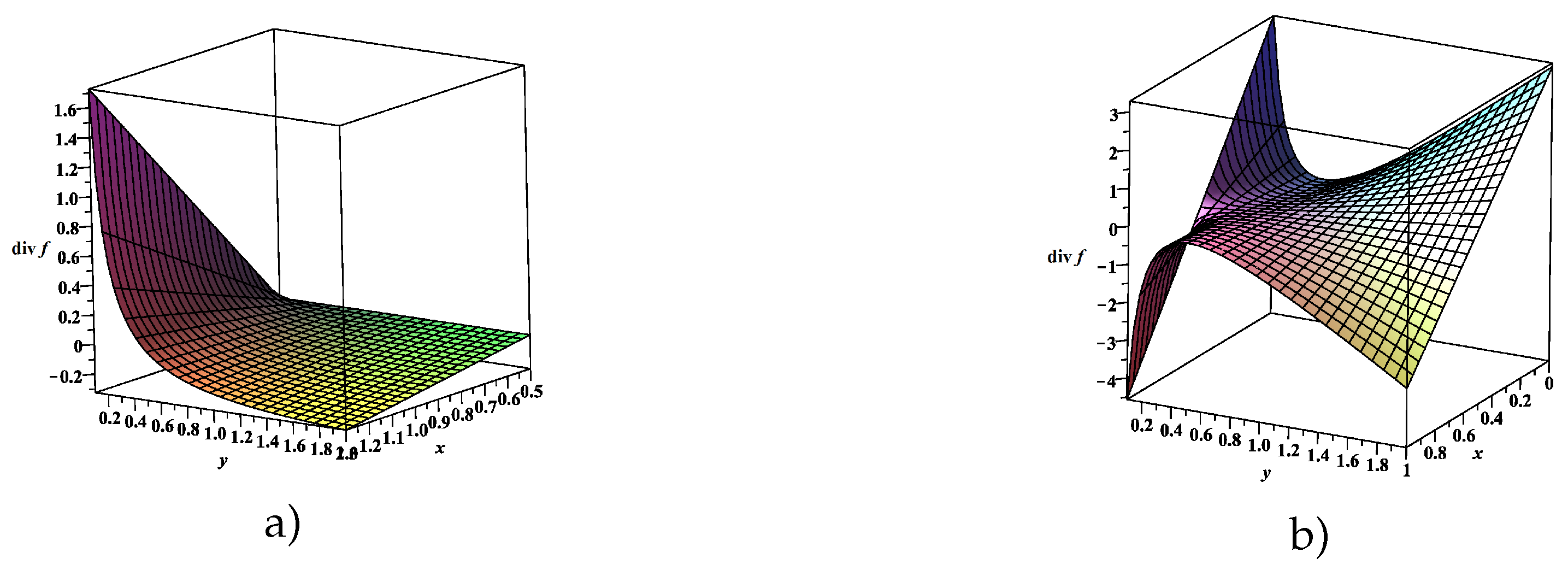
Figure 3 shows examples of simply connected regions in which the divergence of the vector field changes its sign:
Figure 3a is the accumulation rate function (
13), and
Figure 3b is the accumulation rate function (
14).
We will seek a solution to problem (
15) using the numerical one-step Adams-Bashforth-Moulton method of the second order of convergence (trapezoidal method). The phase trajectories obtained according to the numerical method for model (
15) are shown in
Figure 4 taking into account dependencies (
13).
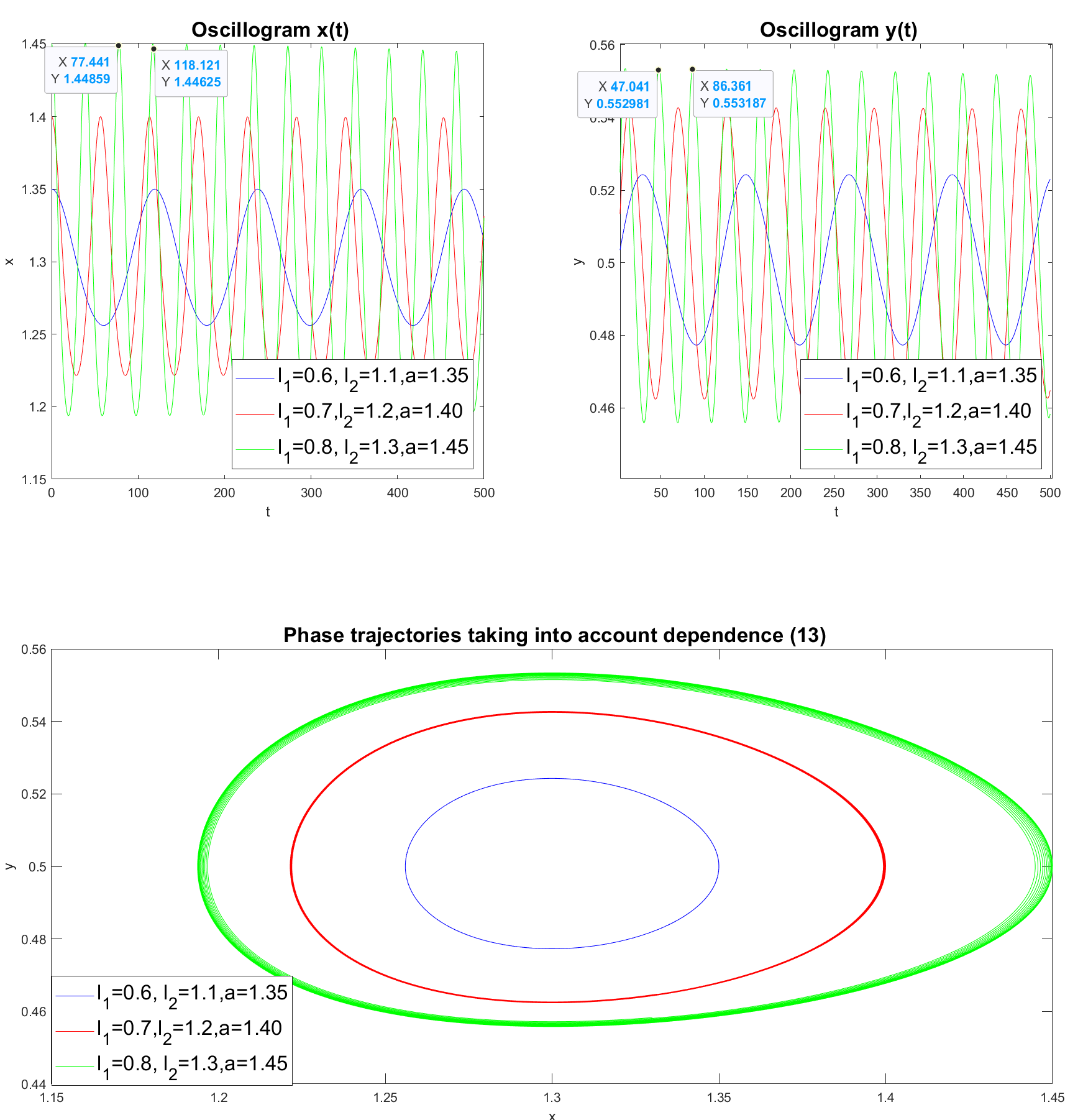
Figure 4 shows the calculation of oscillograms and phase trajectories for the dependence (
13) of the accumulation rate on capital productivity, taking into account different values of
and
a. It can be noted that, in contrast to
Figure 4c, the accumulation rate enhances the asymmetry of the cycle. It can also be noted that an increase in the values of the parameters
affects the frequency and, consequently, the oscillation period. Let the time axis be number of years. Then, for example, we see that for the set of values:
period fluctuations are
years. Indeed, for the efficiency of new technologies
:
years, and for the efficiency of capital productivity
:
39.32 years. This period value corresponds to that indicated by A.A. Akaev. in article [
26], in which the author claims that the duration of N.D. cycles. Kondratieva was on average 40 years old in the 20th century.
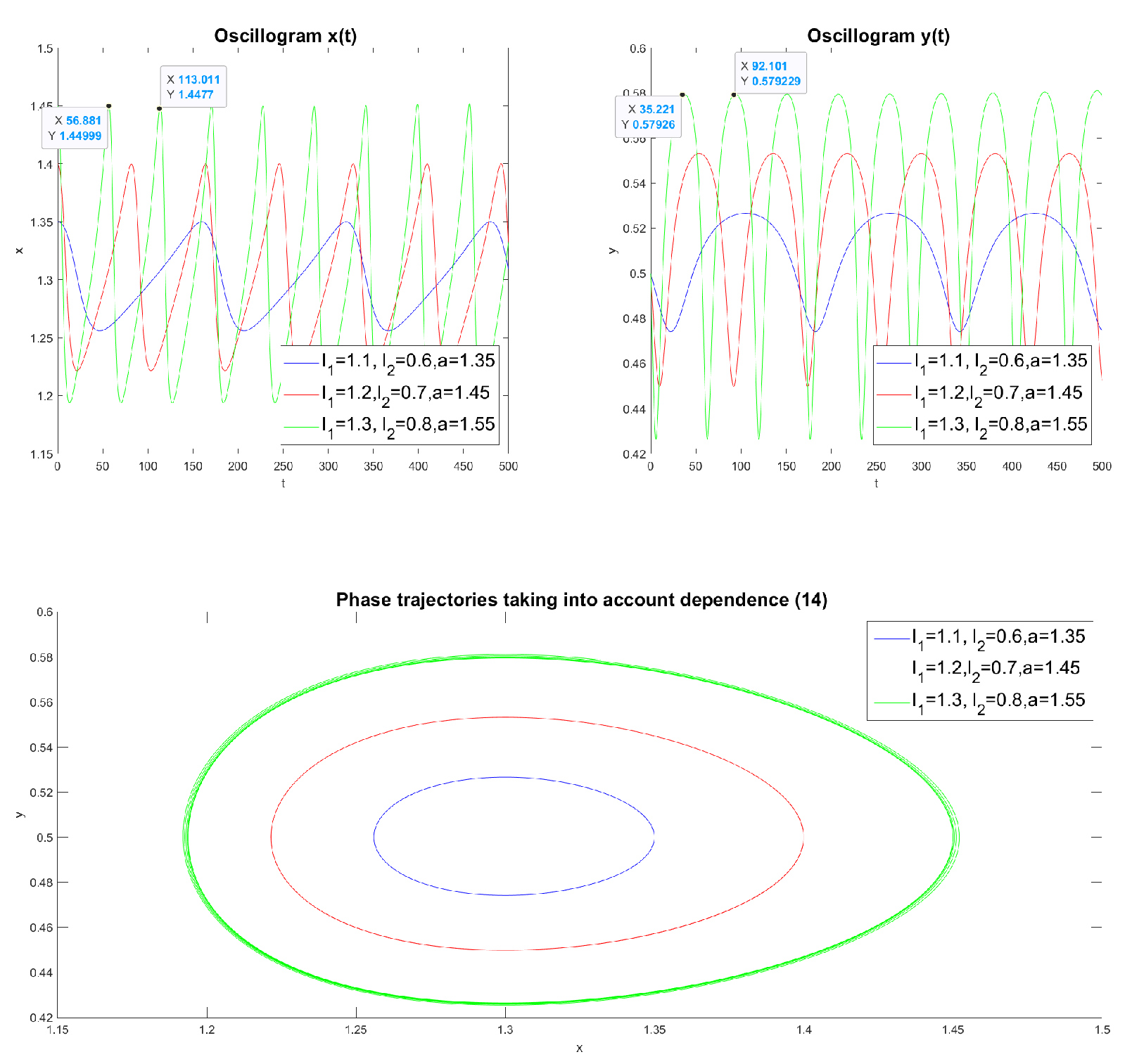
Figure 5 shows the calculation of oscillograms and phase trajectories for dependence (
14) for various values of
and
a.
We see that the phase trajectories are closed. The oscillograms in
Figure 5 differ from the oscillograms in
Figure 4 however, the phase trajectories have similar orbits. Here, too, an increase in the values of
and
a leads to greater cycle asymmetry, which is also reflected in the oscillation period. The oscillation period, for example, for a cycle with parameters
is ≈ 56 years. Such values of oscillation periods were obtained by S.V. Dubovsky in his work [
14], however, these values were somewhat overestimated compared to the real economic cycle. However, despite this, all of the above indicates that the period of a particular cycle can be estimated based on dependencies (
13) and (
14), i.e., with the correct choice of parameter values
and
. Let us remember that the values of these parameters are taken from statistics.
In the case when the selected parameter values give an incorrect value for the cycle period, it is necessary to refine the model. For example, take into account some properties of the system under consideration. As such, external influences on the system (
10) can be taken into account, which determines the influx of external investments and new technologies or management decisions.
2.4. Influx of external investments and new technologies
The influx of external investments and new technologies can be taken into account in the mathematical model (
15) by introducing the functions
and
into its right-hand sides
Remark 10. The mathematical model (16) describes forced nonlinear fluctuations in the efficiency of new technologies and capital productivity.
Remark 11. In our work we will consider the harmonic functions and in model (16), where and are amplitudes, and and are frequencies. The choice of such dependencies is due to the fact that the influx of external investments and new technologies is periodic. In addition, such dependences lead to the occurrence of resonance effects in the oscillatory system, which is of great practical importance. In this work we will demonstrate these properties using computer simulation.
Using the Adams-Bashforth-Moulton numerical algorithm of the second order of convergence for solving the Cauchy problem (
16), we can construct oscillograms and phase trajectories for various values of its parameters, taking into account dependence (
13).
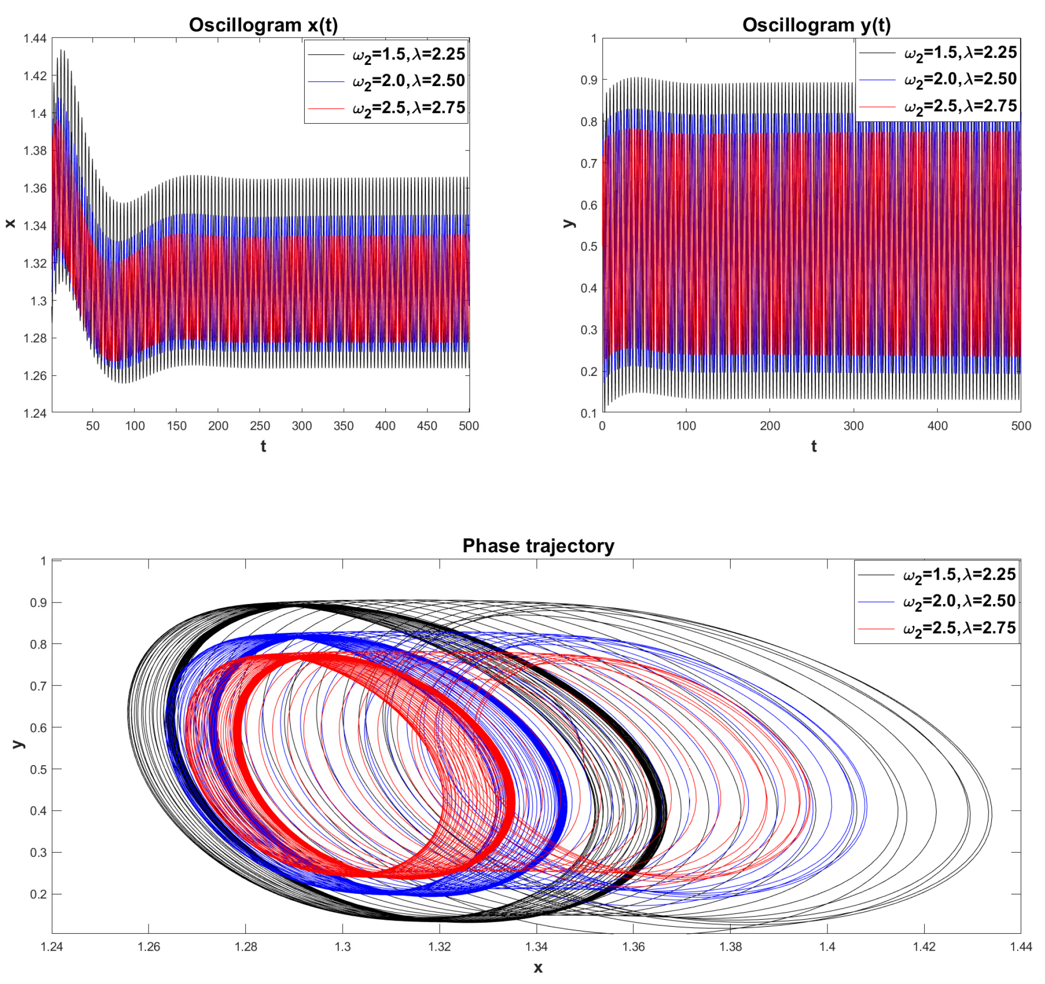
In
Figure 6 shows an example of constructing oscillograms and a phase trajectory obtained with the following parameter values:
,
,
,
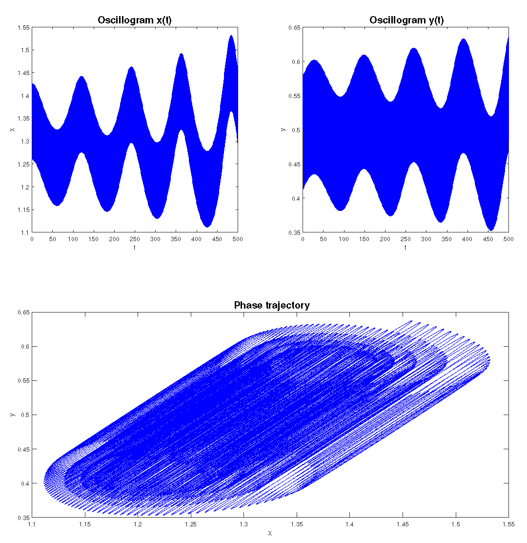
. Note that the phase trajectory is closed; in addition, it experiences oscillations due to external harmonic functions.
Figure 7 shows another example with amplitude values
, other parameters remained unchanged. Here we see on the oscillograms an increase in the amplitude of natural oscillations. The phase trajectory is not closed and has the appearance of an unwinding spiral. Just like in
Figure 7, the phase trajectory experiences oscillations due to external harmonic functions.
For dependence (
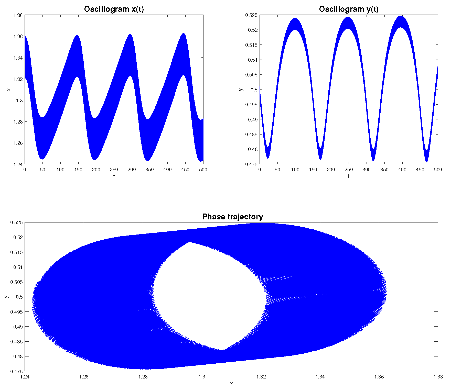
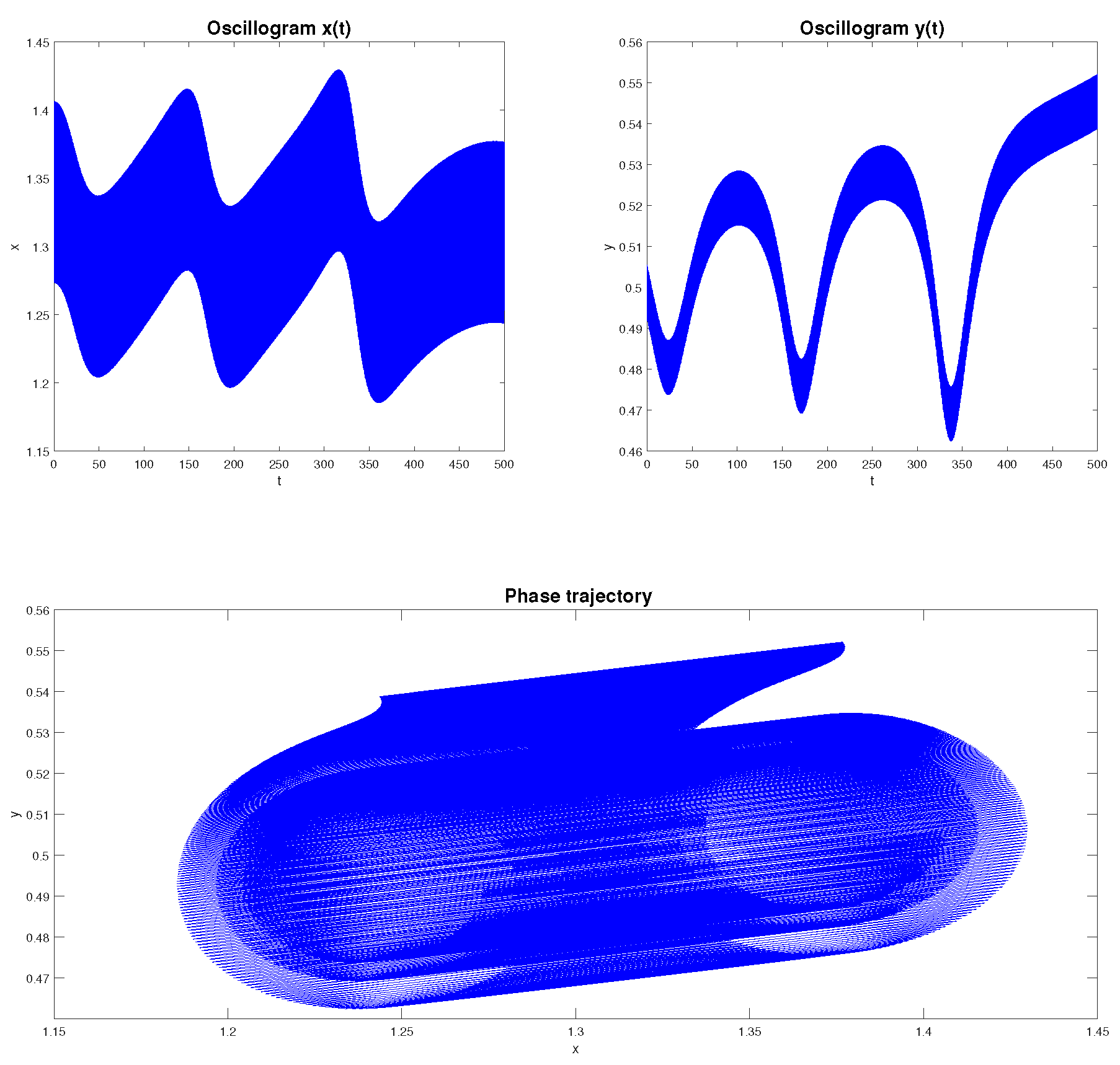
14), both cyclic oscillations (
Figure 8) and resonance effects (
Figure 9) can also occur.
In
Figure 9 we see that the phase trajectory is not closed, it unwinds due to the fact that the amplitude of oscillations increases under resonance conditions. In addition, the trajectory itself experiences vibrations due to external harmonic influence.
In
Figure 6,
Figure 7,
Figure 8 and
Figure 9 it seems that the phase trajectory is a three-dimensional figure. This is due to the fact that the boundary of the phase trajectory also experiences oscillations and time
t here becomes the third degree of freedom.
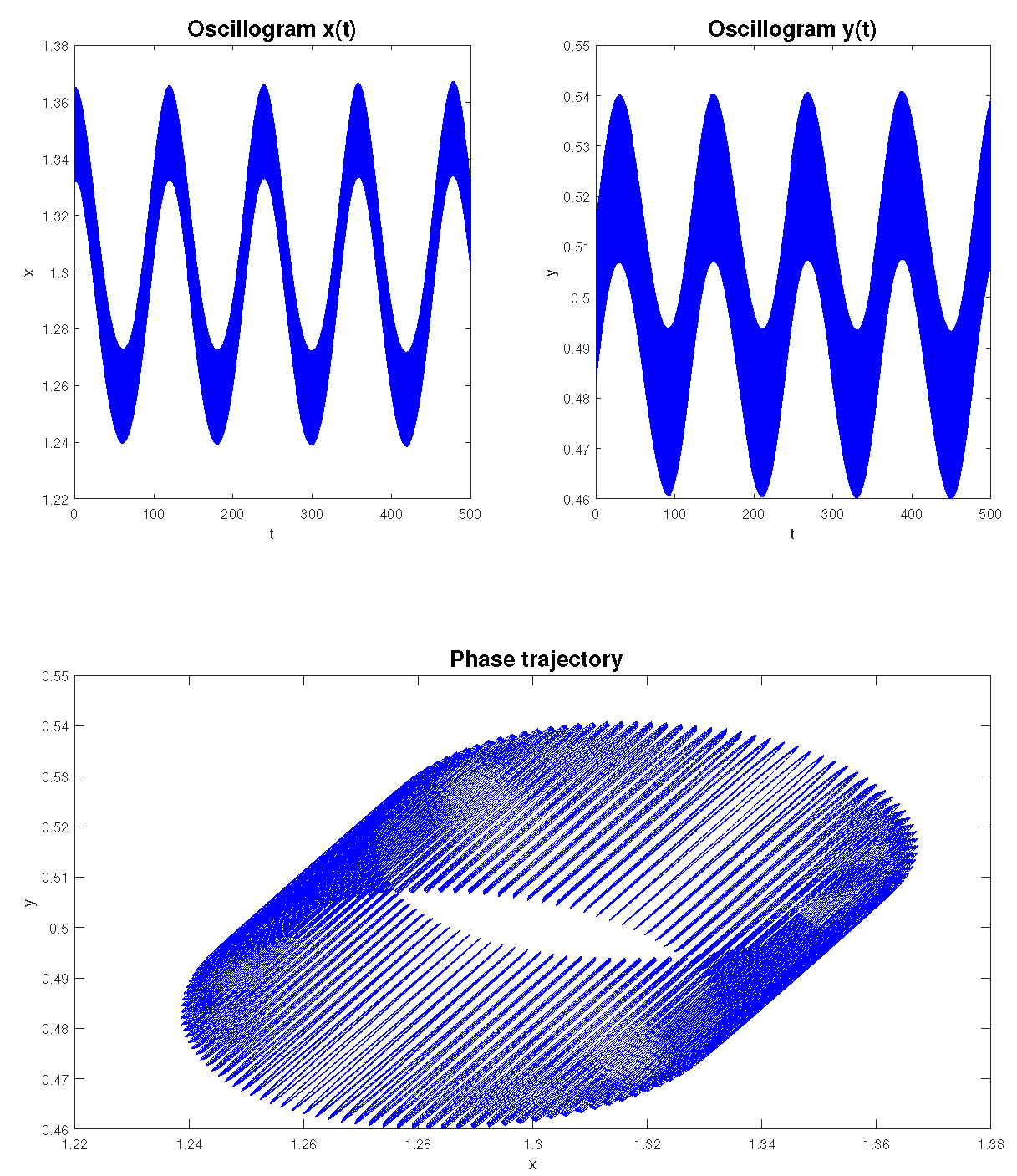
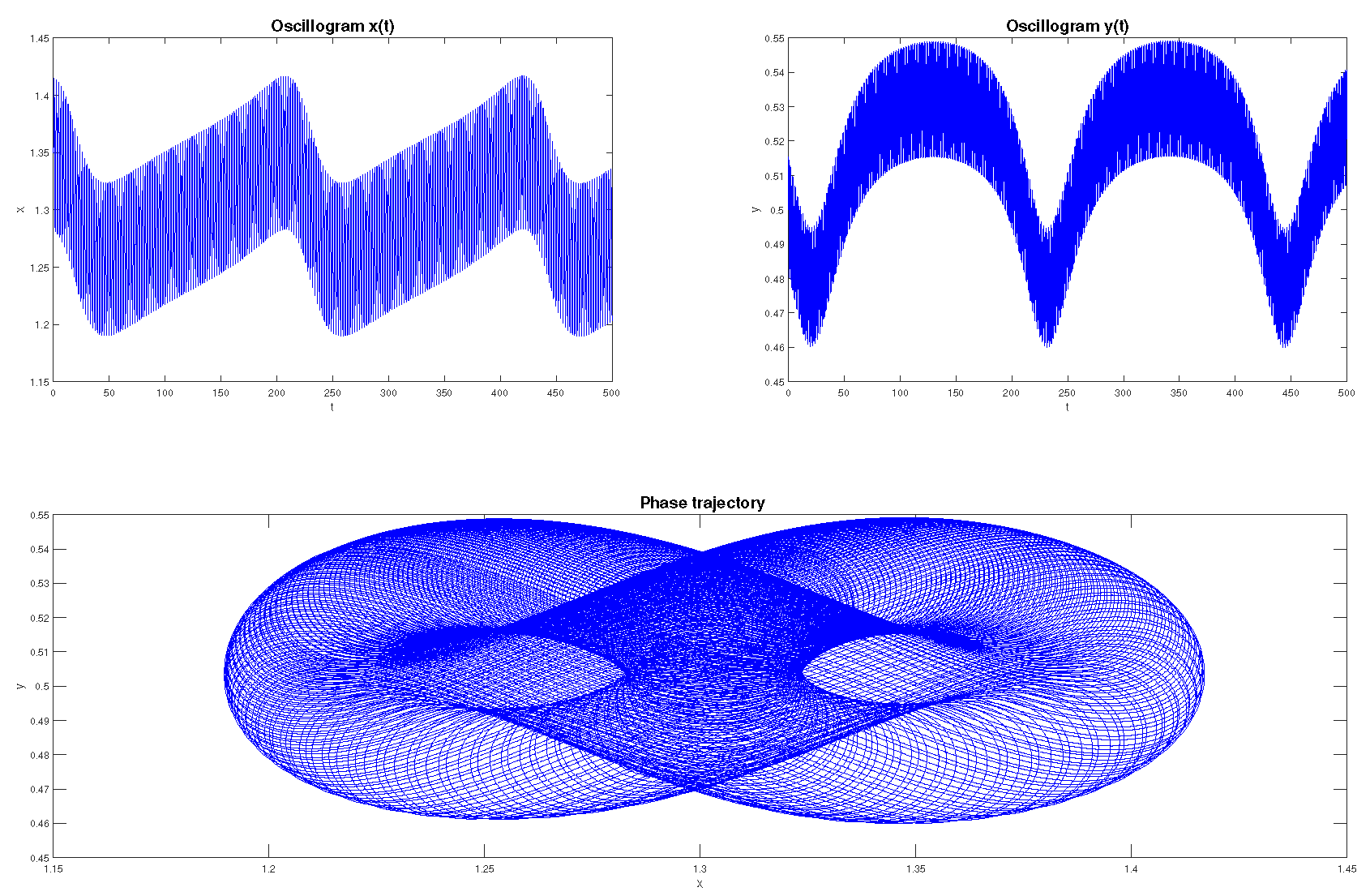
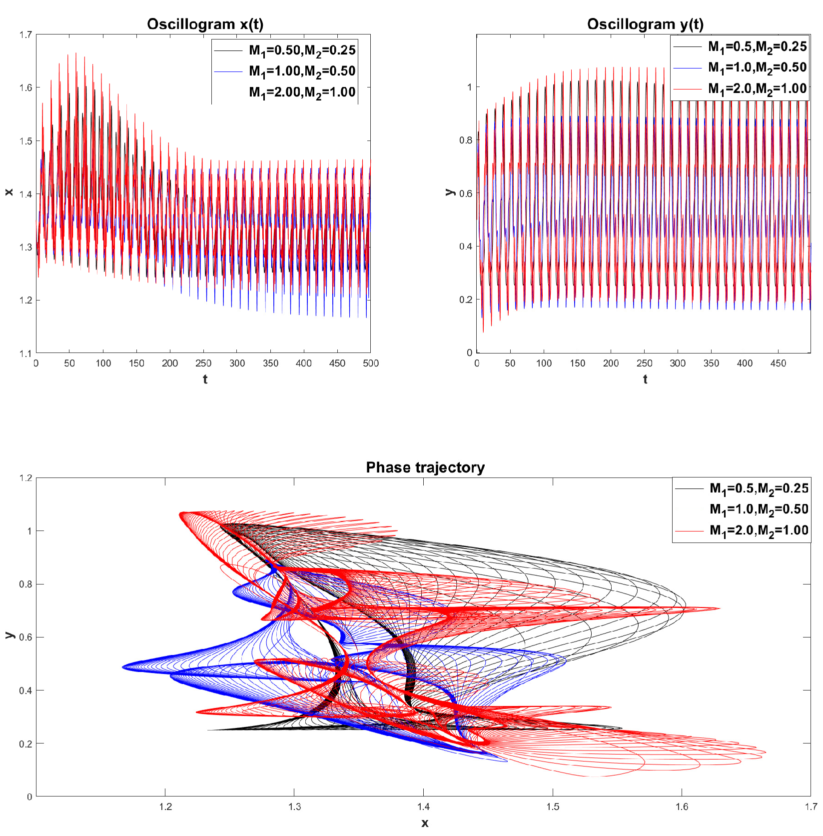
It should be noted that the functions
and
can produce more complex cycles (
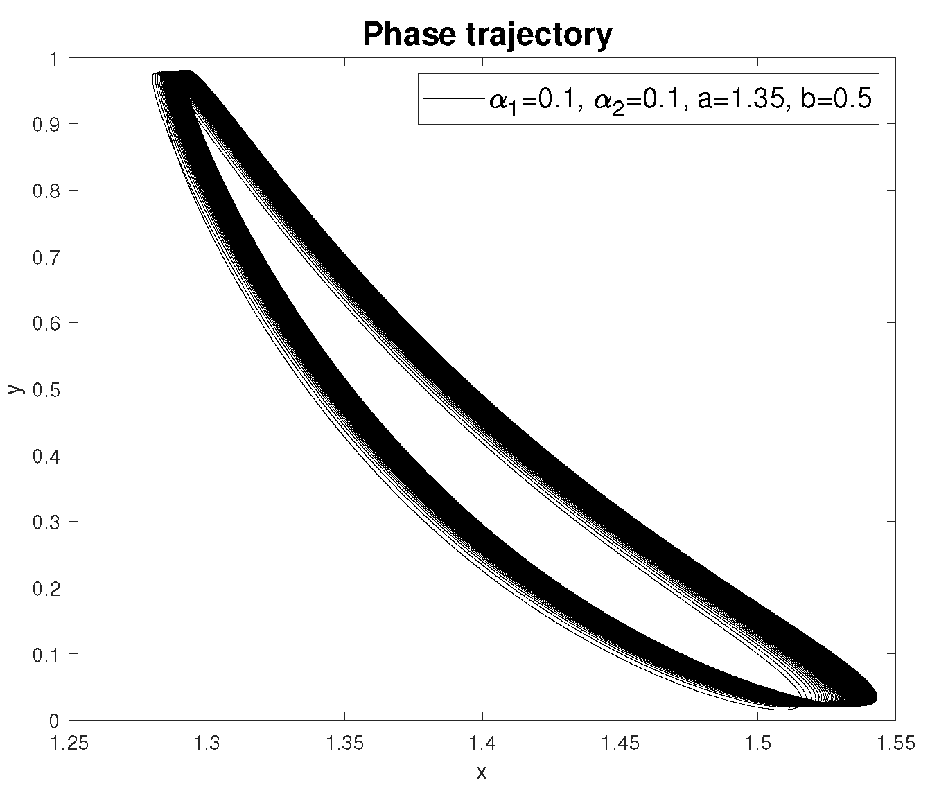
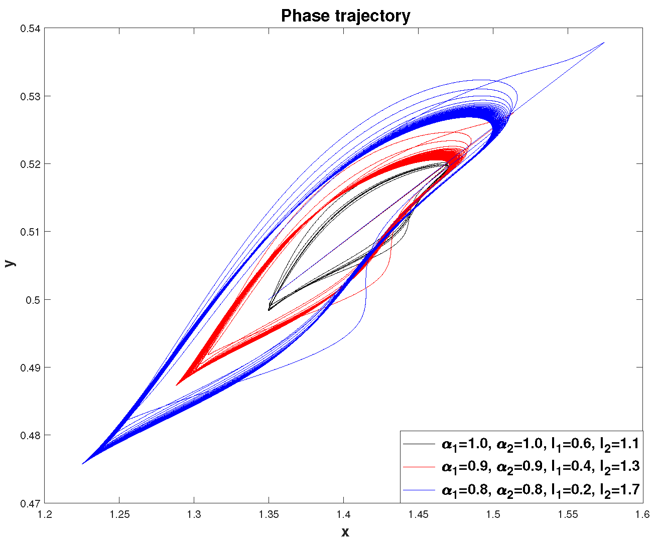
Figure 10).
These complex cycles are similar to Lissajous figures, the shape of which is determined by the ratio of the frequencies and . It is known that if the frequency ratio is a rational number, then the trajectory will be closed, and if it is irrational, then it will not be. In any case, the study of such figures deserves attention.
In the works of the authors [
30,
31,
32,
33,
34], a generalization of the CMMD was proposed taking into account the heredity effect [
54]. This property indicates that the system remembers the impact exerted on it and, from a mathematical point of view, it can be described using integro-differential equations or using a fractional derivative [
37,
38,
39,
40,
41].
It is shown in [
31] that the introduction of fractional derivatives into system (
10) leads to damped oscillations and therefore, in order for cyclic oscillations to exist, it is necessary to have an external source of harmonic form
and
. This makes it possible for the phase trajectory to reach a limit cycle after some time. Let’s consider these modifications of the CMMD (
16).
3. Fractional mathematical model S.V. Dubovsky with constant heredity
In this section we will consider a generalization of the CMMD (
16) in the case of constant heredity using the apparatus of fractional calculus. Let us consider the formulation of the problem in terms of Gerasimov-Caputo fractional derivatives. Next, a solution technique based on the numerical ABM algorithm will be given. The errors of the method are investigated, and an assessment of the computational accuracy using Runge’s rule is given. A visualization of the simulation results and their interpretation, as well as a software implementation of the numerical algorithm are presented.
3.1. Some definitions from the theory of fractional calculus
It should be noted that more detailed information about fractional calculus can be found in well-known monographs [
37,
38,
39,
40,
41].
Definition 3.
Euler’s gamma function is defined:
Definition 4.
Let . Integral
where , is the Euler gamma function (17), called the Riemann-Liouville fractional integral.
The fractional Riemann-Liouville integral (
18) has the following properties:
Definition 5.
The Gerasimov-Caputo fractional derivative of constant order of the function has the form:
where is the Euler gamma function (17).
The Riemann-Liouville fractional integral (
18) and the Gerasimov-Caputo fractional derivative (
20) have the semigroup property:
Remark 12.
It should be noted that operator (20) began to be called Caputo’s fractional derivative and denoted as , thanks to articles [55,56]. This mathematical construction was presented by the Italian mathematician M. Caputo in 1967 in work [57]. However, earlier the Soviet mechanic A.N. Gerasimov in 1948, in his work [58], devoted to plasticity problems within the framework of hereditary mechanics [59], introduced a partial fractional derivative of the order :
Therefore, we will call the fractional derivative operator (20) the Gerasimov-Caputo fractional derivative.
Remark 13. Note that the listed formulas (18) and (20) are valid for functions of many variables. In this case, we will work with partial derivatives of fractional order.
Remark 14. There are other definitions of fractional derivatives and integrals. Some are modifications of the Riemann-Liouville or Gerasimov-Caputo operators. Others are defined differently. The question of choosing one or another fractional operator to solve an applied problem is open. Fractional operators are usually chosen for simplicity in mathematical transformations and interpretation of simulation results. For example, for an equation with the Gerasimov-Caputo operator, traditional initial and boundary conditions are set, which is important for physical applications. The Riesz operator is convenient for the Fourier integral transform.
3.2. Problem statement and solution method
Let’s consider a generalization of the CMMD (
16), which according to (
20) can be represented as the following Cauchy problem:
Remark 15. Note that in the limiting case when we move from the Cauchy problem (22) to the classical Cauchy problem (16).
Remark 16. We will call the Cauchy problem (22) the fractional mathematical model of S.V. Dubovsky (FMMD).
We will not dwell here in detail on the derivation of the model equations in (
22). We will indicate only some approaches. The first approach is to use the semigroup property (
21) [
60]. For example, if the Cauchy problem is written in general form:
Then, act on the first equation (
23) on the left with the operator
, and for the second equation — on
, then we arrive at the problem Cauchy form (
22) with specific functions
and
.
The second approach is based on the formal replacement of integer derivatives from the right side of system (
16) with derivatives of fractional orders [
61]:
where
are parameters that have time dimensions; they are necessary to comply with the dimensions in the model equations. You can always introduce the characteristic time of the process, perform dimensionlessness and, in principle, arrive at system (
22).
There is an approach associated with hereditary (hereditary) equations, in the terminology of Vito Volterra [
54]. For example, we can write the original Cauchy problem in the integro-differential formulation:
where
and
are difference kernels or heredity functions. Further, according to Volterra’s hereditary principles, the memory functions in (
25) should decay as
. So based on this, we can select memory functions as follows:
Substituting relation (
26) into system (
25) taking into account (
20), we can obtain system (
22).
Remark 17. Note that in [62] it is noted that if the memory function is chosen in the form , where ω is a positive constant, is the Dirac function, then we get the absence of memory by analogy with the Markov process. The case when in a dynamic system the memory function has the form , where is the function Heaviside, leads to systems with complete memory availability. The power-law nature of memory functions in the form (26 leads to dynamic systems with “partial loss of memory”.
Due to the nonlinearity of the Cauchy problem (
22), to solve it it is necessary to use numerical methods. We will use the one-step Adams-Bashforth-Moulton method, adapted for solving fractional order differential equations. For the Cauchy problem (
22), a generalization of the numerical ABM method is proposed [
63,
64,
65]. To do this, we introduce a uniform finite-difference grid with a constant step
, as well as grid functions:
,
, ,
,
, for
. A modification of the ABM method takes the following form. For the predictor we get the calculation formulas:
Then, using the Adams-Moulton formula for the corrector, we get:
where the weighting coefficients in (
28) are determined by the formula:
Remark 18. Formulas (27) and (28) with values transform into formulas for the classical ABM method.
3.3. Error analysis of the Adams-Bashforth-Moulton method
This section presents lemmas and the error theorem for the modified ABM method (
27), (
28), more detailed proofs of which can be found in [
63].
Lemma 1.
If the function , then the following estimate holds [63]:
where ||∞|| — Chebyshev norm, .
Lemma 2.
If the function , then there is a constant that depends only from α such that [63]:
Based on Lemma 1 and Lemma 2, we formulate the following theorem.
Theorem 3.
If [64] and
where and are constants, then the Adams-Bashforth-Moulton numerical method converges with the order
Remark 19. Note that in the case when we have the second order of convergence according to estimate (33), which corresponds to the order of convergence of the classical ABM method.
Next, using test examples, we will evaluate the computational accuracy of the ABM method (
27), (
28) using Runge’s rule (double recalculation method) [
66]. For these purposes, we introduce the following calculation formulas:
where
is the theoretical order of accuracy of the ABM method according to estimate (
32),
,
— error of the ABM method,
— numerical solution at step
,
— numerical solution at step
. The computational accuracy
p will then be determined by the formulas:
where
computational grid steps,
,
— solution errors at step
.
Example 1. (Case of CMMD).
Let’s consider a test example in the case . We choose the parameter values for the Cauchy problem (22) as follows: , . The results of the numerical analysis are shown in Table 1.
From
Table 1 it is clear that with an increase in the calculated grid nodes, the computational accuracies
tend to
— the order of accuracy of the classical ABM method.
Example 2. (Case of FMMD).
Let’s consider the case , take the remaining parameters from the previous example. The simulation results are shown in Table 2.
From
Table 2 it is clear that with an increase in the calculated grid nodes, the computational accuracies
tend to
— the order of accuracy of the ABM method (
27), (
28).
3.4. Simulation results
Let’s look at some examples of simulation results within the FMMD model and their visualization. The construction of oscillograms and phase trajectories was carried out using the HFMD 1.0 computer program written in Phyton [
33].
Example 3. (Case of CMMD).
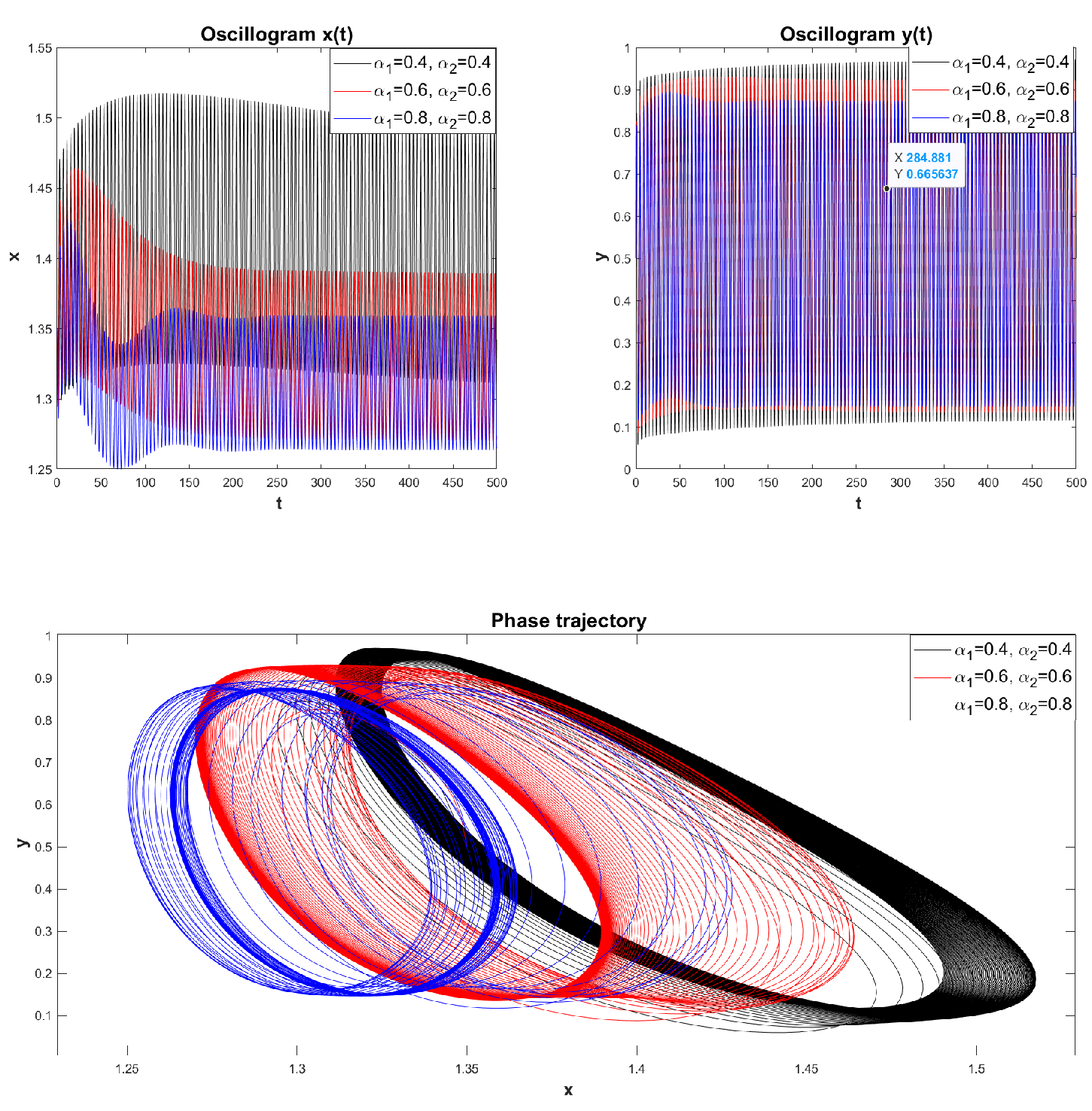
Let’s consider the case when in the numerical ABM algorithm (27), (28) the parameter values are: , and n is a constant. This leads us to model (10), which was considered by S.V. Dubovsky in his work [14]. Let’s choose the values of the remaining parameters: , . Next, using the numerical ABM algorithm (27), (28), we construct oscillograms and phase trajectories for various values of and .
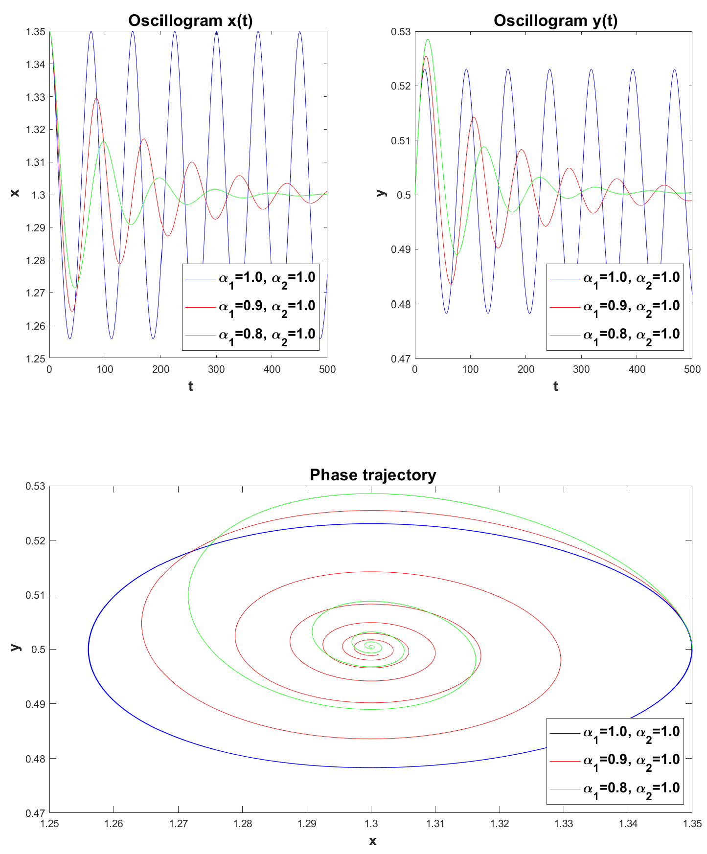
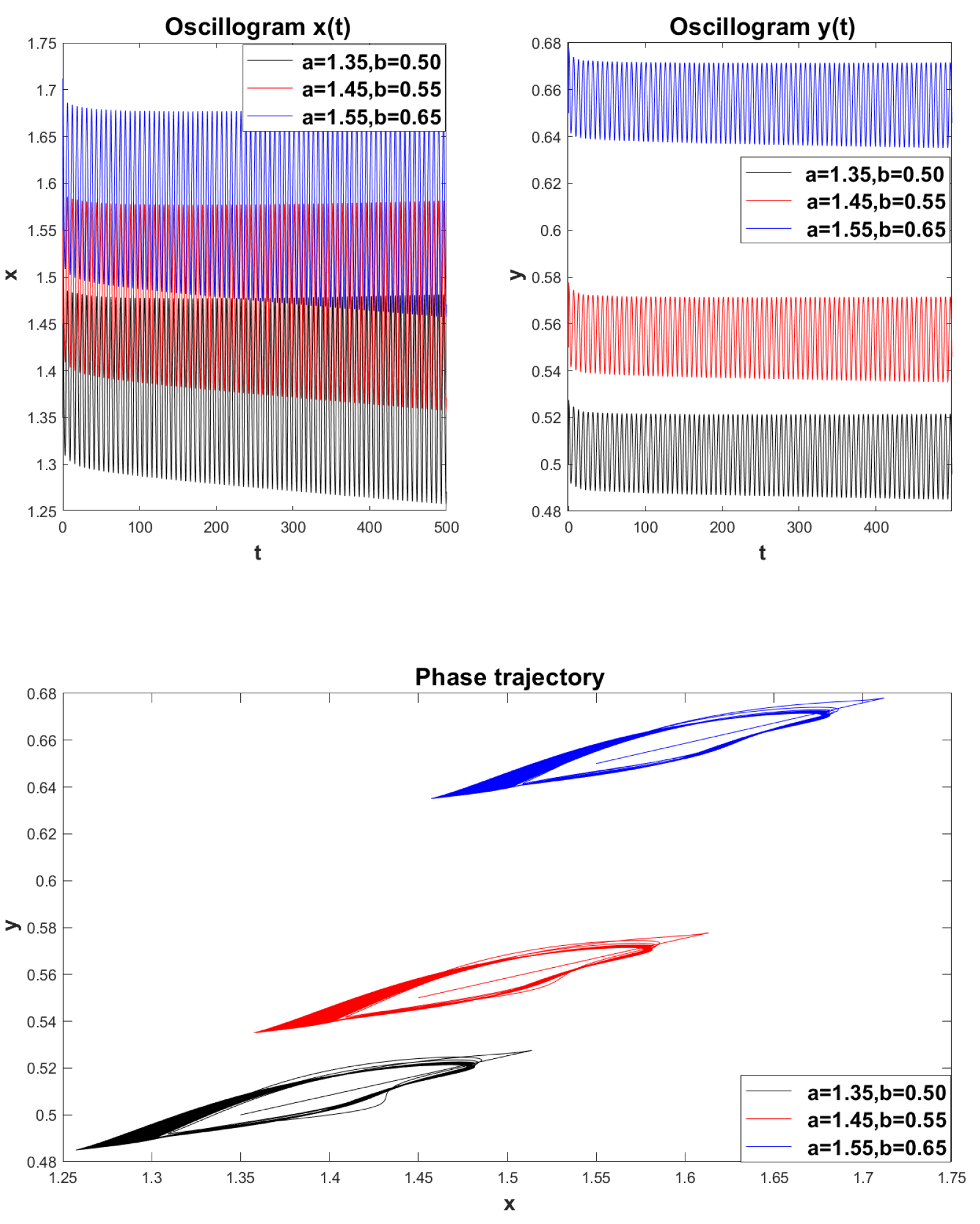
We see that in
Figure 11. the results coincided with the previously obtained results in
Figure 2. This once again confirms that the fractional mathematical model of S.V. Dubovsky is a generalization of the classical mathematical model [
14].
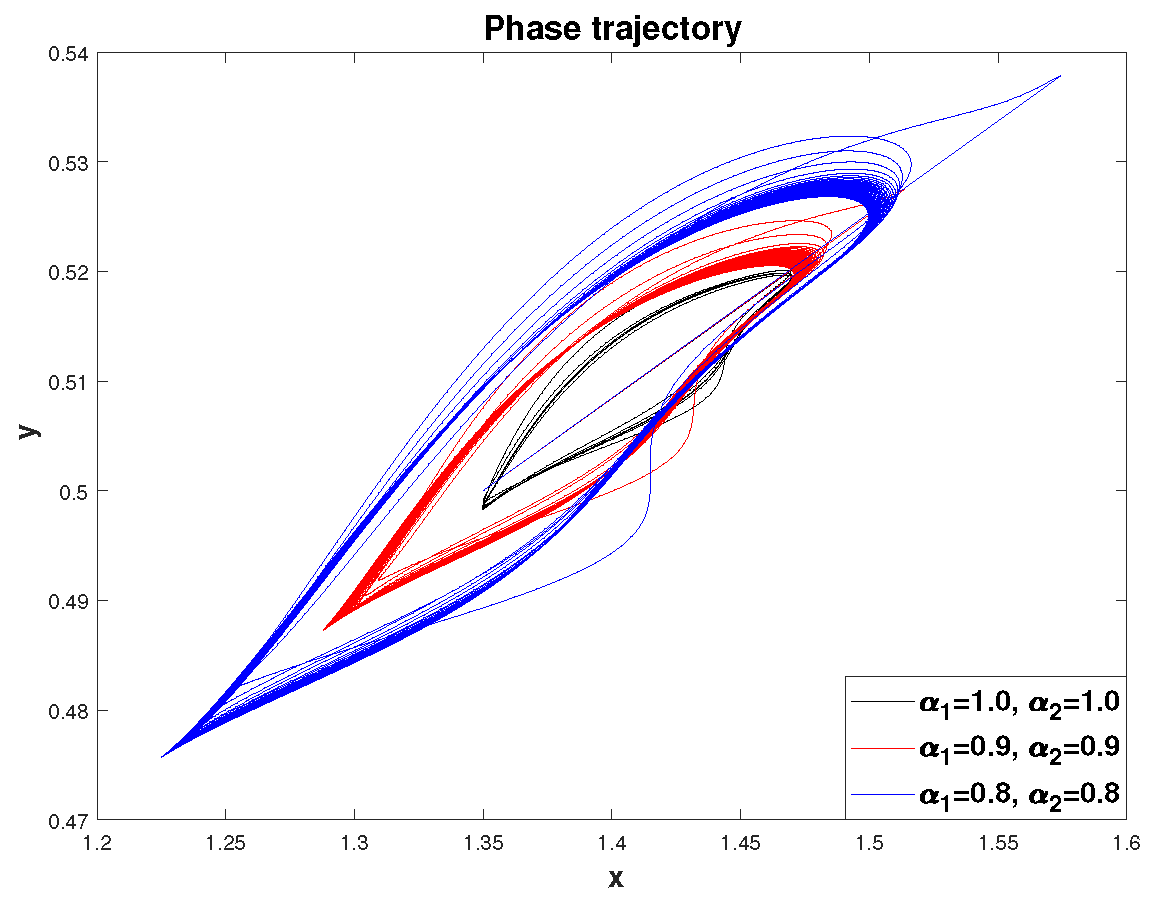
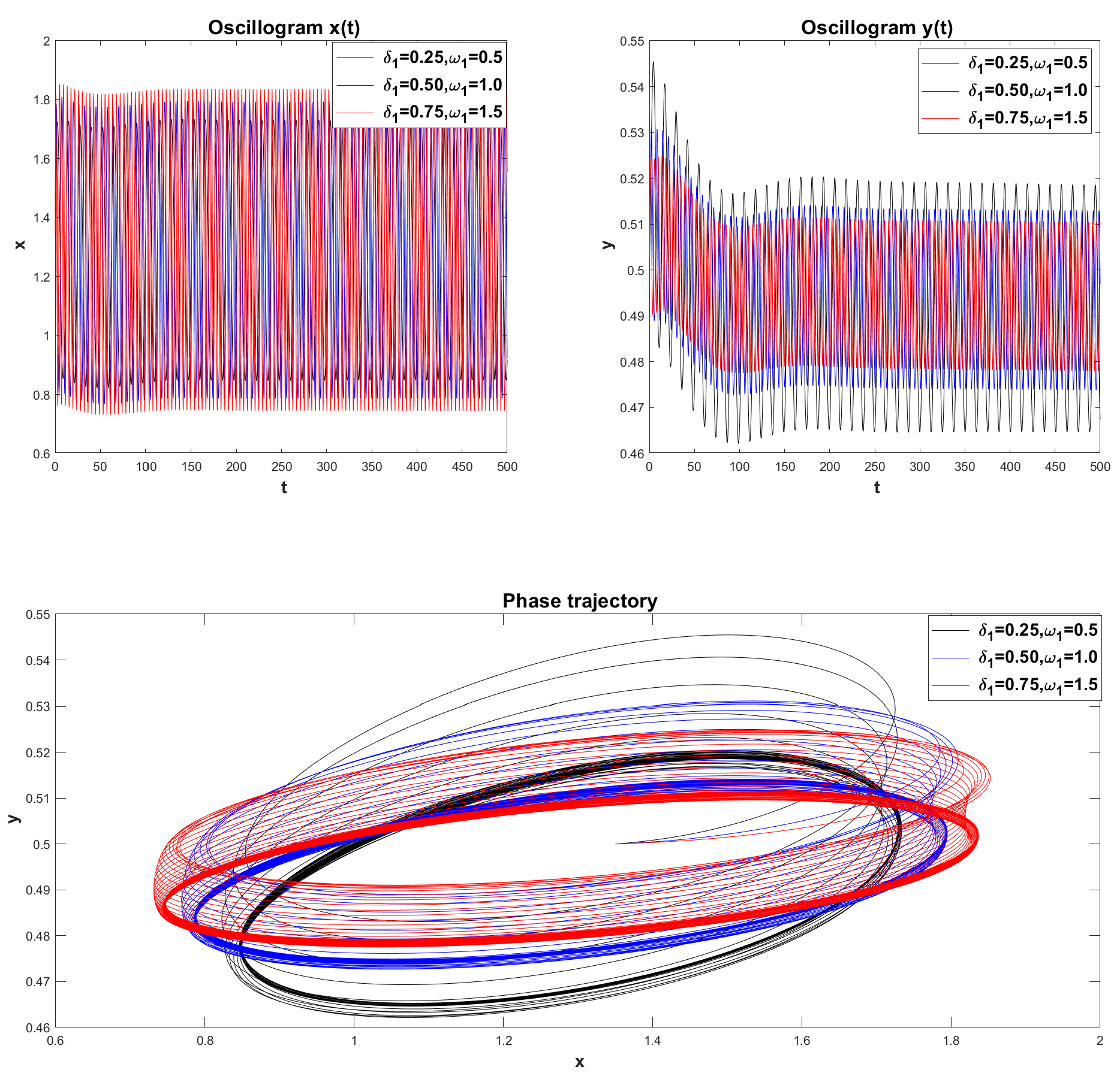
Example 4. (Case of FMMD). Let and , , . In this case, the oscillatory system experiences its own vibrations. Let us construct oscillograms and phase trajectories for various values of with a fixed value of .
In
Figure 12 we see that as the values of the parameter
decrease, the oscillations damp (dissipation) and on the phase plane the rest point
is a stable focus. Let’s give another example. Let’s fix the value
and change the values
.
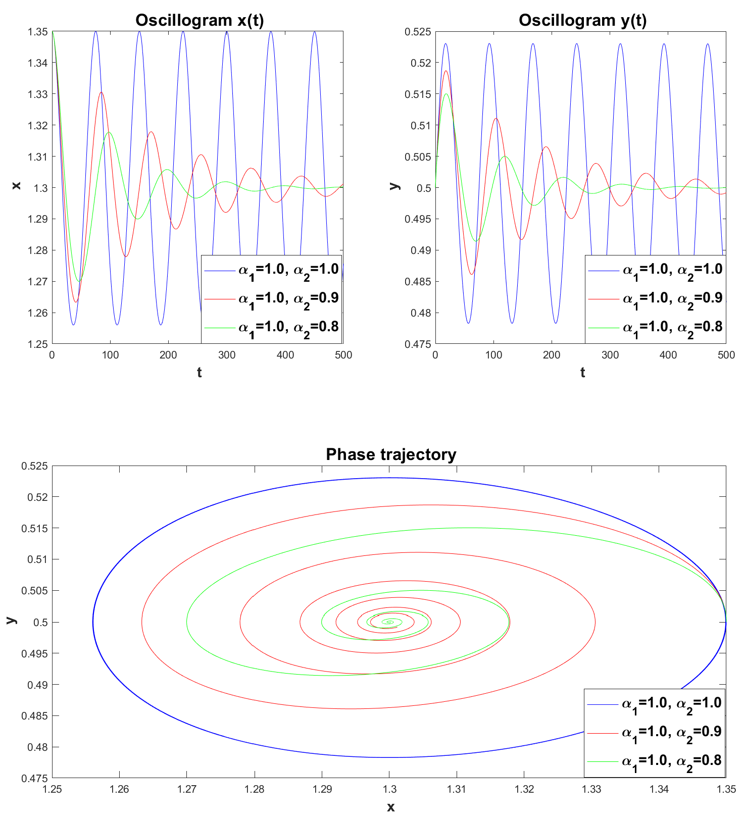
Here is the same as in
Figure 12, in
Figure 13. we see damped oscillations when changing the values of the parameter
, rest point
is also a stable focus (phase trajectories — twisting spirals).
Based on the damped oscillatory mode, we can conclude that the presence of memory in system (
22), provided there is no external influence, does not lead to a closed phase trajectory, i.e., There is no self-oscillating mode in the system. Therefore, the existence of a closed trajectory is possible only under external influence. Let us now consider an example taken from [
32].
Example 5. Fractional mathematical model S.V. Dubovsky with parameter values [29]: , , , , .
It can be noted that the phase trajectory in
Figure 14 here goes to the limit cycle. Let us construct phase trajectories depending on different values of the initial conditions.
Figure 15 shows a family of phase trajectories obtained for different initial values of
. These phase trajectories show that the limit cycle presented in
Figure 14 is not stable.
Definition 6. A limit cycle is called stable if all phase trajectories starting in the ε-neighborhood asymptotically approach the limit cycle as . Limit cycles in which close phase trajectories approach them indefinitely are called attractors. Limit cycles in which close phase trajectories repel from them are called repellers.
Indeed, if we take the initial values inside this limit cycle, for example, the value
, then the phase trajectory goes to another limit cycle with a larger orbit – the red phase trajectory in
Figure 15. Next, we can see that with a further increase in the initial value along the x-axis and a decrease in the initial value along the ordinate axis, we get another limit cycle again with a larger orbit — the blue phase trajectory in
Figure 15.
Example 6. Fractional mathematical model S.V. Dubovsky with comparable parameter values: . We will select the values of the remaining parameters from Example 5.
Figure 16 shows a visualization of the simulation results for various parameter values:
. We see that all phase trajectories reach limit cycles. As the values of the parameters
and
decrease, the limit cycles have an increasingly larger orbit. In addition, we see that as the values of the parameters
and
decrease, the time to reach the limit cycle also increases. This indicates that a memory effect occurs in system (
22), i.e., It takes time to stabilize the oscillatory modes.
Let’s consider the following more general case (
Figure 17). Let’s choose the parameter values:
, and leave the remaining parameters unchanged.
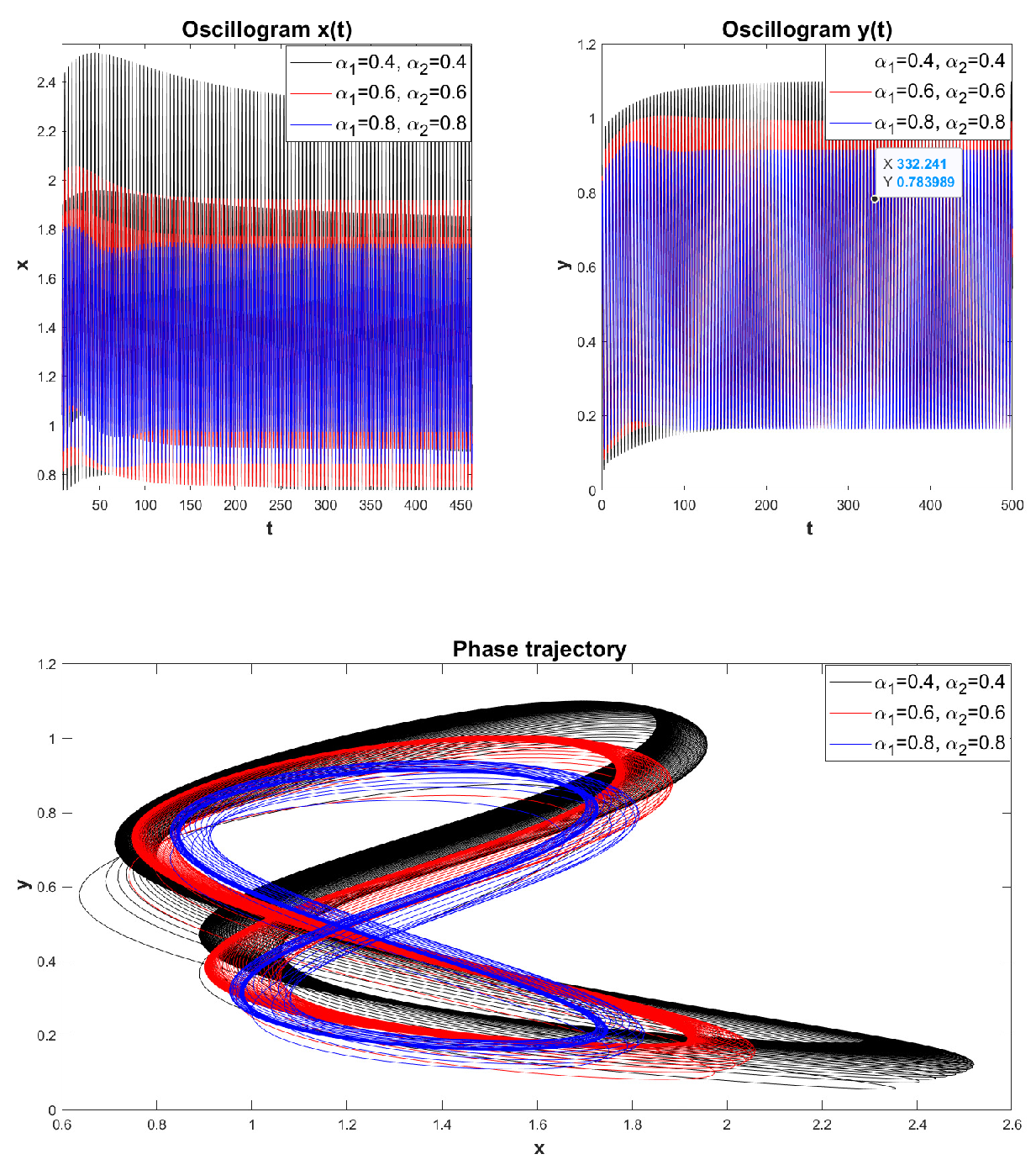
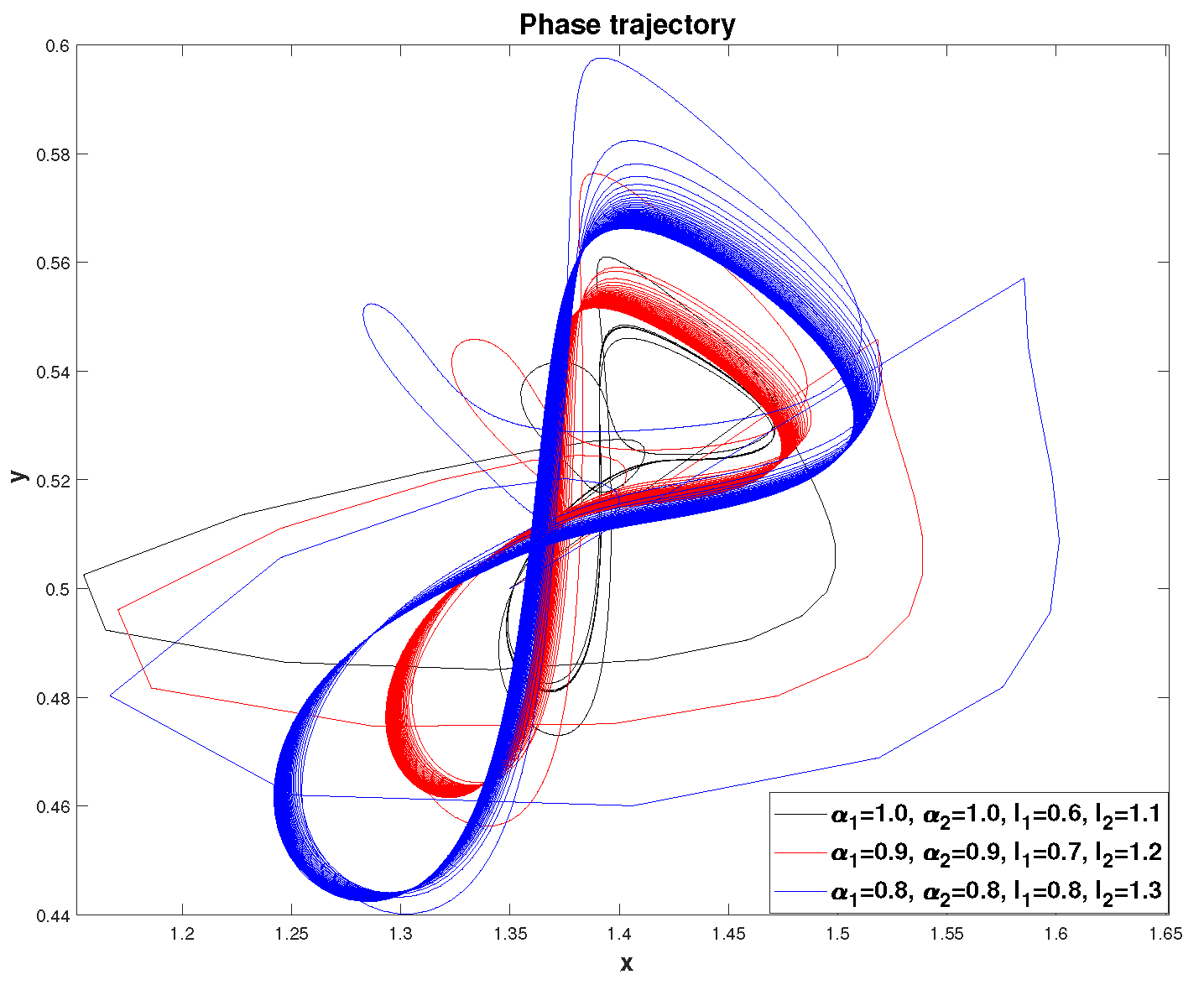
The presence of external influence in the form of harmonic functions, taking into account heredity, significantly complicates the nature of oscillations and the shape of phase trajectories (
Figure 17). The shape of the phase trajectories is more similar to Lissajous figures, which are found in technology and depends on the frequency ratio
. However, due to the memory effect, these figures are quite strongly deformed, for example (see
Figure 10). We also see that the trend from previous examples remains the same: as the values of
and
decrease, the time to reach the limit cycle increases, as well as its orbit .
Let us now consider the fractional mathematical model of S.V. Dubovsky, when the accumulation rate
n is a function of capital productivity
and changes according to law (
13), where
and
. Let us construct phase trajectories for various values of
and
. The values of the remaining parameters will be left unchanged.
We see that when external influence is turned on with parameter values
,
the phase trajectories reach the limit cycle. Note that the shape of limit cycles differs from those previously obtained; this is due to the influence of the accumulation rate as a function of capital productivity. Moreover, this inversely proportional relationship (
13), the greater the capital productivity, the lower the accumulation rate. Here you can also notice that the efficiency of new technologies
and the efficiency of fixed assets
behave the same way: they either increase together or decrease together.
Figure 19 shows the phase trajectories for various values of the parameters
, as well as
and
. We will take the remaining parameter values from the previous example. It can be seen that in this case the general trend continues, as in the previous case. However, we see that the phase trajectories are different here: they are more deformed and the orbits are more enlarged. In
Figure 18 and
Figure 19, from an economic point of view, you can notice the following: first, the system needs to reach the limit cycle for some time; at the limit cycle there is a simultaneous increase in the efficiency of new technologies and the efficiency of fixed assets; after some time, there is a simultaneous decline in these indicators, which intensifies as a result of an increase in the accumulation rate; the latter means that the growth of capital productivity is slowed down and its decline is accelerating.
In
Figure 20 shows another example of constructing a phase trajectory for the values of the parameters
with fixed values of
and
for dependence (
14). Here we see that the phase trajectories reach a limit cycle similar to
Figure 17. Such limit cycles deserve special attention and economic interpretation.
4. Fractional mathematical model S.V. Dubovsky with variable heredity
This section proposes the next stage of modernization of FMMD — taking into account variable heredity. This means that the economic system in question has memory effects that change over time. From a mathematical point of view, the change in memory over time can be described using derivatives of fractional order variables.
4.1. Definition of fractional derivative of variable order
Fractional derivatives of variable orders are studied within the framework of the theory of fractional calculus. There is a well-known review article [
67], in which the authors covered in more detail various definitions of the derivative of a fractional variable order and its applications. As one of the applications, we can cite the article [
68], where a description of the financial system was given using a derivative of a fractional variable order.
Definition 7.
Fractional derivative of variable order of Gerasimov-Caputo type for , :
where is a known function from the class .
Remark 20. In the case when in definition (36) the function is a constant, then we come to the definition of the Gerasimov-Caputo fractional derivative (20).
Remark 21. Similarly, one can introduce the definition of a fractional integral of variable order of the Riemann-Liouville type, as for constant order (18). However, it should be noted here that the semigroup property between the variable-order fractional derivative operators and the variable-order fractional integral is violated [69,70].
4.2. Problem statement and solution method
Based on Remark 21 and taking into account Definition 7, we can write the following Cauchy problem:
Remark 22. Note that in the case when the functions and are constants, then the Cauchy problem (37) becomes the Cauchy problem (22).
Remark 23. We will call the Cauchy problem (37) the fractional mathematical model of S.V. Dubov variable order (FMMD VO).
Methods for numerical analysis of equations with derivatives of fractional order variables are quite well developed, some of them can be studied in articles [
71,
72,
73,
74].
For the Cauchy problem (
37), a generalization of the numerical ABM method (
27), (
28) is proposed [
70]. To do this, we introduce a uniform finite-difference grid with a constant step
, as well as grid functions:
,
,
,
,
for
. A modification of the ABM method takes the following form:
Then, using the Adams-Moulton formula for the corrector, we get:
where the weighting coefficients in (
39) are determined by the formula:
4.3. Error analysis of the modified Adams-Bashforth-Moulton method
In this section we present lemmas and a theorem, which are a generalization of the results from
Section 3.3 Proofs of lemmas and theorems are carried out similarly to the method proposed in
Section 3.3 [
68].
Lemma 3.
If the function , then the following estimate holds:
where ||∞|| — Chebyshev norm, .
Lemma 4.
If the function , then there is a constant , which depends only on such that:
Theorem 4.
If and
then the ABM method (38) and (39) converges with the order
Let us evaluate the computational accuracy of the ABM method (
38), (
39) using Runge’s rule (
34) and (
35, which is compared with the theoretical one. Good agreement between them was obtained. In the test examples, we used linearly monotonically decreasing functions
and
of the form:
where
are given constants whose values satisfy the inequalities
.
From the
Table 3 we see that the computational accuracy approaches the theoretical
q in three iterations according to the ABM method (
38), (
39).
Example 7. . The theoretical order of convergence of the ABM method: .
Example 8. , , . The theoretical order of convergence of the ABM method: .
From the
Table 4 we see that the computational accuracy approaches the theoretical
q in five iterations according to the ABM method.
According to Examples 7 and 8, we can conclude that the estimate of the computational accuracy tends to the theoretical one within a finite number of iterations of the ABM method. The latter indicates the adequacy of estimate (
44).
4.4. Simulation results
Let’s visualize the simulation results for different parameter values. To do this, we will use procedures written in MATLAB, which are included in the FDDSVO computer program (
Appendix A).
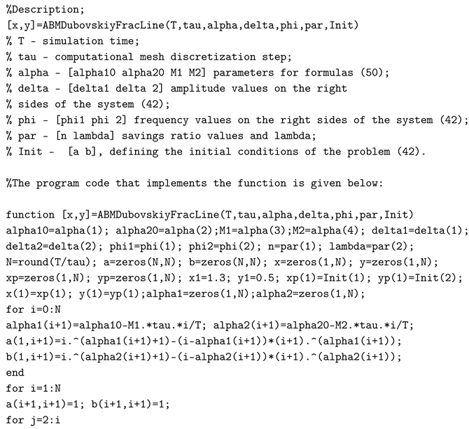
Example 9. Let us consider the case when the orders and of fractional derivatives linearly decrease on according to formula (45) [33]. Parameter values: , , , , , , . For mathematical modeling we choose: .
To find a numerical solution to system (
37), a function was written in MATLAB (
Appendix A.1) [
33] which outputs oscillograms and phase trajectories based on the numerical solution of system (
37) using the ABM method (
38), (
39). Application of function for different values of parameters
and
, which are included in formulas (
45).
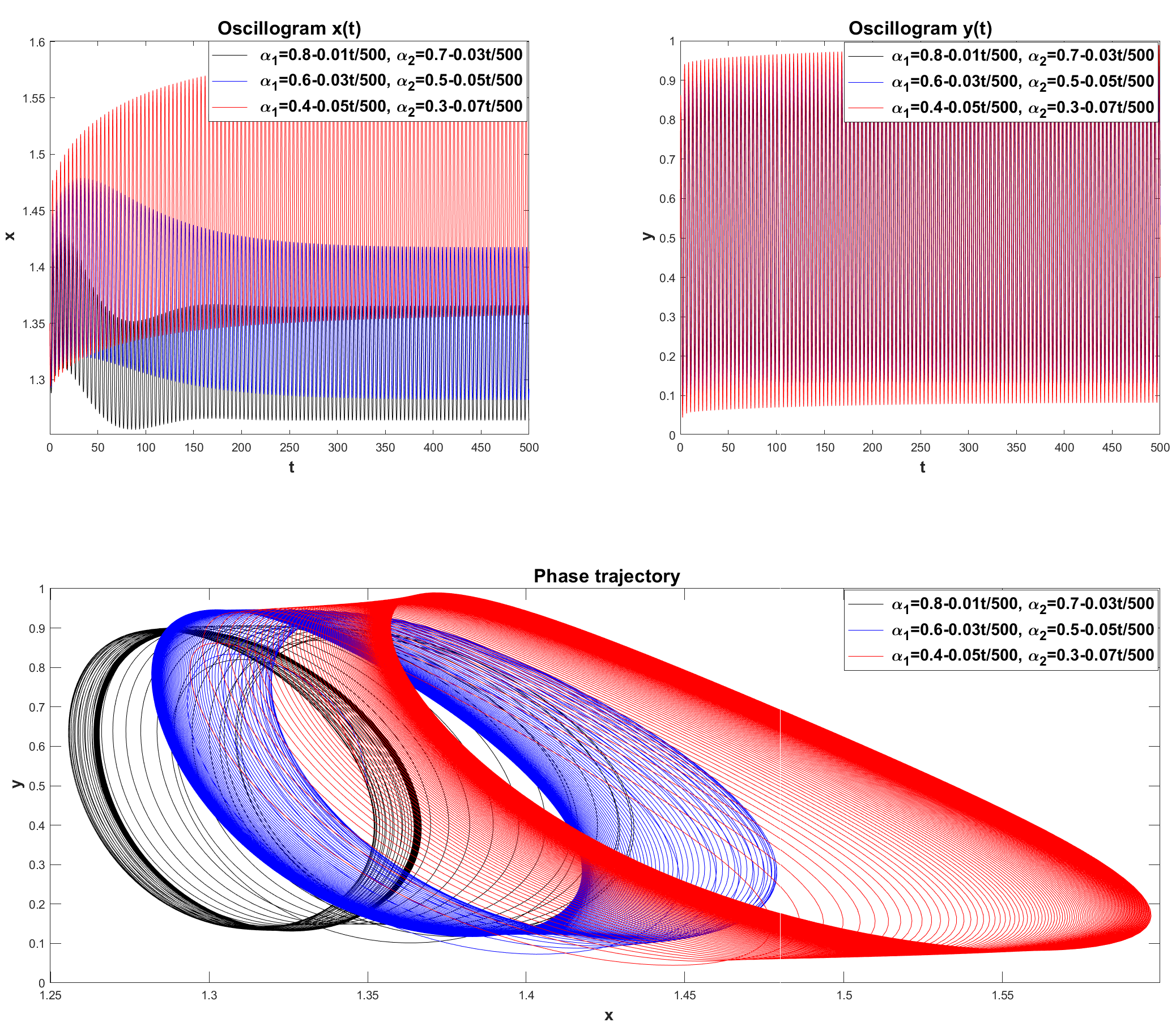
In
Figure 21 show oscillograms for Example 9. Here we can observe that over time the oscillations reach a constant level, and the rest point
for the corresponding closed phase trajectory is called limit cycle. It can be noted that as the values of
and
decrease, the exit time increases to the limit cycle, and the orbit of the limit cycle itself becomes larger.
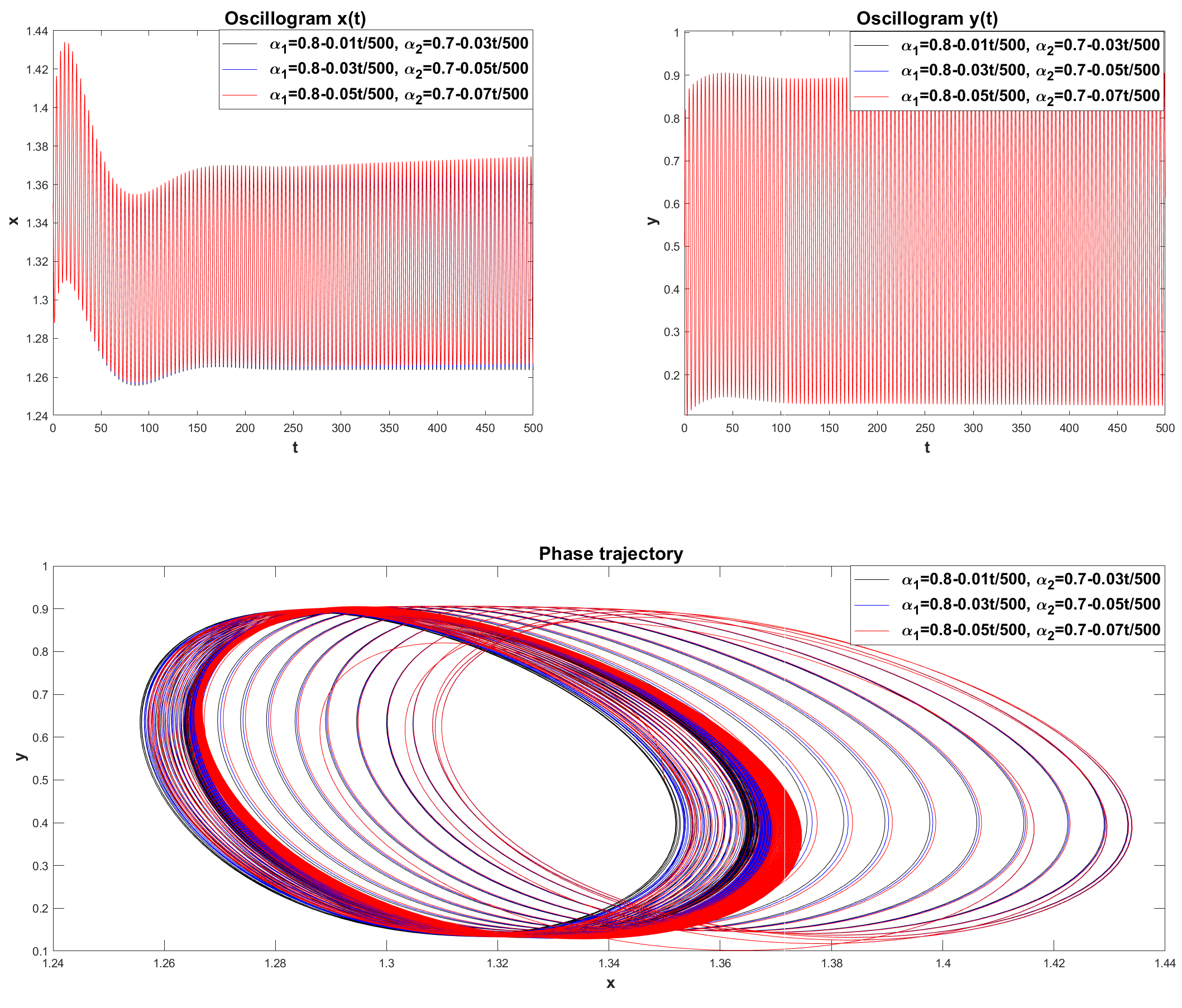
In
Figure 22 we see that the phase trajectories reach limit cycles, which are located quite close to each other. Let’s consider the case when the parameter values are:
,
,
,
are fixed in formula (
45), and the values of the parameters
and
vary.
In
Figure 23 we see that increasing the values of the parameter
and the frequency of external influence
leads to a decrease in the orbits of limit cycles. Let’s consider the case when the parameters
and
change (
Figure 24).
Here we also see that the phase trajectories become closed over time. Let’s consider the case for Example 9, when the initial conditions of system (
37) change.
In
Figure 25 we see that the phase trajectories reach a stable limit cycle.
In Example 9 the accumulation rate coefficient
n was constant. Let’s consider an example when the accumulation rate is a function of capital productivity
according to relation (
14).
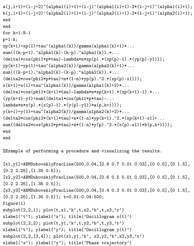
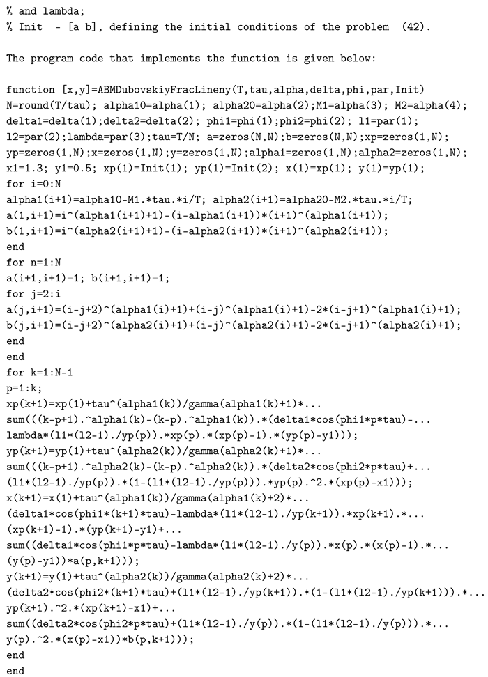
Example 10. Let us consider the case when relations (14) and (45) are satisfied. We will take the parameters for modeling from the previous Example 9. The function that implements the numerical algorithm for solving the fractional system (37) taking into account (14) and (45) can be represented in MATLAB as the function ABMDubovskiyFracLineny.m (see Appendix A.2) . Let’s consider the case when in relation (14) the values , , and the remaining parameters are taken from the previous Example 9. The values of the parameters and in formulas (45) change.
We see in
Figure 26 that the limit cycles have a complex shape and are strongly deformed as the values of
and
increase. An interesting case is when the values of the parameters
and
change. The type of functions is presented below.
In
Figure 27 shows oscillograms and phase trajectories for Example 10 with parameter values
and
. Here we also see the exit of the phase trajectory to the limit cycle.
To conclude this example, we present the case when the initial conditions
a and
b change (
Figure 28).
5. Conclusions
In conclusion, the following conclusions can be drawn from the research results. Mathematical models have been developed taking into account constant and variable heredity, which generalize the previously known classical model of S.V. Dubovsky to describe long waves N.D. Kondratiev within the framework of the interaction between the effectiveness of new technologies and the efficiency of capital productivity. These models are based on a system of nonlinear ordinary differential equations with derivatives of fractional constant and variable orders, which are understood in the Gerasimov-Caputo sense with corresponding local initial conditions. In addition, the models took into account the rate of accumulation as a function of capital productivity and external inflow of investment and new technologies. Using the Bendixson criterion, it is shown that the classical model of S.V. Dubovsky can have closed trajectories.
Numerical algorithms have been developed to search for solutions to the proposed mathematical models based on the Adams-Bashforth-Moulton method from the family of predictor-correctors. For such methods, an error analysis was carried out, the results were formulated in the form of lemmas and theorems. Next, using test examples and Runge’s rule, estimates of the accuracy of calculations were obtained, which gave good agreement with the theoretical results.
Computer experiments were carried out using the proposed numerical algorithms. Oscillograms and phase trajectories were constructed for various values of the model parameters. It is shown that in the absence of external influence, the fractional mathematical model of S.V. Dubovsky oscillations are only damped, i.e., there are no self-oscillations. The presence of external influence makes possible the existence of a limit cycle, which may not always be stable. The limit cycle can be greatly deformed if the orders of fractional derivatives are functions of time, and the shape of the limit cycle can also be influenced by the function of the rate of accumulation from capital productivity. Complex oscillatory regimes deserve separate study and, accordingly, economic interpretation.
It should be noted that further development of the mathematical models proposed in this article may consist in taking into account the dependence of the orders of fractional derivatives not only on time, but also on the solution function by analogy with the article [
75]. Another direction of research is related to the qualitative analysis of dynamic regimes and the construction of their maps by analogy with the article [
76].
Author Contributions
Conceptualization, R.P. and D.M.; methodology, R.P.; software, D.M.; validation, R.P. and D.M.; formal analysis, R.P.; investigation, D.M.; resources, D.M.; writing—original draft preparation, D.M. and R.P.; writing—review and editing, D.M. and R.P.; visualization, D.M.; supervision, R.P. All authors have read and agreed to the published version of the manuscript.
Funding
The work was carried out within the framework of a framework agreement on cooperation for 2022-2027 between the Institute of Cinematography, Far Eastern Branch of the Russian Academy of Sciences and the National University of Uzbekistan named after Mirzo Ulugbek No. 1118 dated 04/28/2022.
Data Availability Statement
The original contributions presented in the study are included in the article, further inquiries can be directed to the corresponding author.
Conflicts of Interest
The authors declare no conflicts of interest.
Abbreviations
The following abbreviations are used in this manuscript:
| CMMD |
Classical Mathematical Model of S.V. Dubovsky |
| ABM |
Adams-Bashforth-Moulton Method |
| FMMD |
Fractional Mathematical Model of S.V. Dubovsky |
| FMMDVO |
Fractional Mathematical Model of S.V. Dubov Variable Order |
6. Listing of FDDSVO program procedures
6.1. ABMDubovskiyFracLine.m
6.2. ABMDubovskiyFracLineny.m
References
- Clarke, H. Physical Economy. A Preliminary Inquiry into the Physical Laws Governing the Periods of Famines and Panics. Railway Register 1847, 5, 155–169. [Google Scholar]
- Juglar, C. Des crises commercials et de leur retour periodique en France, en Angleterre et aux EU; Guillaumin: Paris, France, 1862; p. 258 p. [Google Scholar]
- Jevons, W. S. The solar-commercial cycle. Nature 1882, 26, 226–228. [Google Scholar] [CrossRef]
- Tugan-Baranovskiy, M. Industrial crises. Essay on the social history of England; O. N. Popova: S.-Pb., Russia, 1900; p. 354 p. [Google Scholar]
- Kitchin, J. Cycles and Trends in Economic Factors. Review of Economics and Statistics 1923, 5, 10–16. [Google Scholar] [CrossRef]
- Kondratyev, N. D.; Oparin, D. N. Large cycles of market conditions; Institute of Economics: Moscow, Russia, 1928; p. 287 p. [Google Scholar]
- Solow, R.M. Technical Change and the Aggregate Production Function. The Review of Economics and Statistics 1957, 39, 312–320. [Google Scholar] [CrossRef]
- Rostow, W. W. Technical The Stages of Economic Growth. The Economic History Review, New Series 1959, 12, 1–16. [Google Scholar] [CrossRef]
- Mensch, G. Stalemate in Technology. Innovations Overcome the Depression; Ballinger Pub Co.: Cambrg., UK, 1979; p. 241 p. [Google Scholar]
- Gattei, G. Every 25 years? Strike waves and long economic cycles. In Proceedings of the colloquium "The Long Waves in the Economic Conjuncture—The Present State of the International Debates", Brussels, Belgium, 12-14 Junuary 1989; pp. 12–14.
- Menshikov, S. M.; Klimenko, L. A. Long waves in economics; International relations: Moscow, Russia, 1989; pp. 145–149. [Google Scholar]
- Amos, Jr O. M. Growth pole cycles: A synthesis of growth pole and long wave theories. Review of Regional Studies 1990, 20, 37–48. [Google Scholar]
- Tylecotte, A. Long Wave in the World Economy: The Present Crisis in Historical Perspective; Psychology Press: London, New York, 1993; p. 338 p. [Google Scholar]
- Dubovsky, S. V. Modeling object Kondratiev cycle. Mathematical modeling 1995, 7, 65–74. [Google Scholar]
- Alexander, M. A. The Kondratiev cycle: A generational interpretation; IUniverse: Bloomington, USA, 2002; p. 314 p. [Google Scholar]
- Kondratiev, N. D.; Yakovets, Yu. V.; Abalkin L., I. Large cycles of conjuncture and the theory of foresight: Selected works; Economics: Moscow, Russia, 2002; p. 766 p. [Google Scholar]
- Hirooka, M. Innovation Dynamism and Economic Growth. A Nonlinear Perspective; Edward Elgar: Cheltenham, Northampton, UK, 2006. [Google Scholar]
- Akaev, A. A. Derivation of the general macroeconomic dynamics equation describing the joint interaction of long-term growth and business cycles. Doklady Mathematics 2007, 76, 879–881. [Google Scholar] [CrossRef]
- Akaev, A. A. Influence of business cycles on long-term economic growth. Doklady Mathematics 2008, 78, 621–625. [Google Scholar] [CrossRef]
- Muller, K. H. Farewell to Long Waves: Substituting Cyclical Approaches in Innovation and Technology Research with a RISC-Framework; University of Ljubljana: Ljubljana, Slovenia, 2008; p. 54 p. [Google Scholar]
- Korotaev, A. V.; Tsirel, S. V. Kondratieff waves in global economic dynamics. System monitoring. Global and regional development; Librocom: Moscow, Russia, 2009; p. 229 p. [Google Scholar]
- Dementyev, V. E. Long waves of economic development and financial bubbles; CEMI RAS: Moscow, Russia, 2009. [Google Scholar]
- Akaev, A. A. Qualitative analysis of business cycles’ influence on economic growth. Economics and mathematical methods 2009, 45, 78–137. [Google Scholar]
- Gladkikh, I. P. Long waves in the post-industrial economy: Theoretical foundations and features; Lambert Academic, Saarbrücken, Germany, 2012.
- Dubovsky, S. V. Modeling Kondratiev cycles and forecasting crises. In Kondratiev waves. Aspects and prospects; Akaev, A. A., Ed.; Uchitel’: Volgograd, Russia, 2012; pp. 179–188. [Google Scholar]
- Akaev, A. A. Mathematical foundations of the Schumpeter-Kondratiev innovation-cyclical theory of economic development. In Kondratiev waves. Aspects and prospects; Akaev, A. A., Ed.; Uchitel’: Volgograd, Russia, 2012; pp. 314–341. [Google Scholar]
- Makarov, D. V.; Parovik, R. I. Modeling of the economic cycles using the theory of fractional calculus. Journal of Internet Banking and Commerce 2016, 21, S21. [Google Scholar]
- Kleinknecht, A. Innovation patterns in crisis and prosperity: Schumpeter’s long cycle reconsidered; Springer: Germany, 2016; p. 235 p. [Google Scholar]
- Kondratyev, N. D. Large cycles of market conditions. Selected works; Yurayt Publishing House: Moscow, Russia, 2021; p. 290 p. [Google Scholar]
- Makarov, D.; Parovik, R. Numerical modeling of Kondratyev’s long waves taking into account heredity. AIP Conference Proceedings 2021, 2365, 020007. [Google Scholar]
- Makarov, D. V.; Parovik, R. I. A computer program for the numerical analysis of economic cycles within the framework of the Dubovsky generalized model. AIP Conference Proceedings 2022, 2467, 060015. [Google Scholar]
- Makarov, D. V.; Parovik R., I. Fractional mathematical model S.V. Dubovsky and economic cycles. Problems of Computational and Applied Mathematics 2023, 52, 8–25. [Google Scholar]
- Makarov, D. V.; Parovik R., I. Fractional mathematical model S.V. Dubovsky with the effect of variable heredity. Problems of Computational and Applied Mathematics 2023, 53, 5–22. [Google Scholar]
- Makarov, D. V. The classical mathematical model of S.V. Dubovsky and some of its modifications for describing K-waves. Vestnik KRAUNC. Fiz.-mat. nauki 2024, 46, 52–69. [Google Scholar]
- Landa, P. S. Regular and chaotic oscillations; Springer: Berlin, Germany, 2012; p. 397 p. [Google Scholar]
- Lichtenberg, A. J.; Lieberman, M. A. Regular and chaotic dynamics; Springer: Berlin, Germany, 2013; p. 692 p. [Google Scholar]
- Oldham, K. B.; Spanier, J. The fractional calculus. Theory and applications of differentiation and integration to arbitrary order; Academic Press: London, UK, 1974; p. 240 p. [Google Scholar]
- Miller, K. S.; Ross, B. An introduction to the fractional calculus and fractional differential equations; A Wiley-Interscience publication: New York, USA, 1993; p. 384 p. [Google Scholar]
- Nakhushev, A. M. Fractional calculus and its application; Fizmatlit: Moscow, Russia, 2003; p. 272 p. [Google Scholar]
- Pskhu, A. V. Fractional partial differential equations; Nauka: Moscow, Russia, 2005; 199 p. [Google Scholar]
- Kilbas, A. A.; Srivastava, H. M.; Trujillo, J.J. Theory and Applications of Fractional Differential Equations; Elsevier: Amsterdam, Golland, 2006; 523 p. [Google Scholar]
- Tarasov, V. E. On history of mathematical economics: Application of fractional calculus. Mathematics 2019, 7, 509. [Google Scholar] [CrossRef]
- Granger, C.W.J. The typical spectral shape of an economic variable. Econometrica 1966, 34, 150–161. [Google Scholar] [CrossRef]
- Granger, C.W.J.; Joyeux, R. An introduction to long memory time series models and fractional differencing. J. Time Ser. Anal. 1980, 1, 15–39. [Google Scholar] [CrossRef]
- Rogers, L.C.G. Arbitrage with fractional Brownian motion. Math. Financ. 1997, 7, 95–105. [Google Scholar] [CrossRef]
- Scalas, E.; Gorenflo, R.; Mainardi, F. Fractional calculus and continuous-time finance. Phys. A Stat. Mech. Its Appl. 2000, 284, 376–384. [Google Scholar] [CrossRef]
- Mainardi, F.; Raberto, M.; Gorenflo, R.; Scalas, E. Fractional calculus and continuous-time finance II: The waiting-time distribution. Phys. A Stat. Mech. Appl. 2000, 287, 468–481. [Google Scholar] [CrossRef]
- Chen, W. C. Nonlinear dynamics and chaos in a fractional-order financial system. Chaos Solitons Fract. 2008, 36, 1305–1314. [Google Scholar] [CrossRef]
- Tarasov, V. E.; Tarasova, V. V. Criterion of existence of power-law memory for economic processes. Entropy 2018, 20, 414. [Google Scholar] [CrossRef]
- Pakhira, R.; Ghosh, U.; Sarkar, S. Study of memory effect in an inventory model with quadratic type demand rate and salvage value. Appl. Math. Sci. 2019, 13, 209–223. [Google Scholar] [CrossRef]
- Bendixson, I. Sur les courbes définies par des équations différentielles. Acta Math. 1901, 24, 1–88. [Google Scholar] [CrossRef]
- Iserles, A. A first course in the numerical analysis of differential equations; Cambridge university press: Cambridge, UK, 2009; 459 p. [Google Scholar]
- Stoleru, L. Economic equilibrium and growth; North-Holland Publishing Company: Amsterdam, Holland, 1975; 300 p. [Google Scholar]
- Volterra, V. Functional theory, integral and integro-differential equations; Dover Publications: New York, USA, 2005; 288 p. [Google Scholar]
- Podlubny, I. Fractional differential equations: An introduction to fractional derivatives, fractional differential equations, to methods of their solution and some of their applications; Elsevier: Amsterdam, Hollan, 1998; 340 p. [Google Scholar]
- Mainardi, F. Fractional calculus and waves in linear viscoelasticity: An introduction to mathematical models; World Scientific: Singapore, 2010; 368 p. [Google Scholar]
- Gerasimov, A. N. Generalization of the laws of linear deformation and their application to problems of internal friction. Academy of Sciences of the SSR. Applied mathematics and mechanics 1948, 44, 62–78. [Google Scholar]
- Caputo, M. Linear models of dissipation whose Q is almost frequency independent – II. Geophysical Journal International 1967, 13, 529–539. [Google Scholar] [CrossRef]
- Rabotnov, Yu. N. Elements of hereditary mechanics of solids; MIR Publishers: Moscow, Russia, 1980; 287 p. [Google Scholar]
- Pskhu, A. V. , Rekhviashvili S.Sh. Analysis of Forced Oscillations of a Fractional Oscillator. Technical Physics Letters 2018, 44, 1218–1221. [Google Scholar] [CrossRef]
- Aguilar, J. F. G.; Hernández M., M. Space-time fractional diffusion-advection equation with Caputo derivative. Abstract and Applied Analysis 2014, 2014, 283019. [Google Scholar] [CrossRef]
- Butenkov, S. A. Mathematical models of processes on fractal structures with given properties based on granulation methods. News of the Southern Federal University. Technical science 2011, 121, 199–209. [Google Scholar]
- Diethelm, K.; Ford, N. J. , Freed A. D. A predictor-corrector approach for the numerical solution of fractional differential equations. Nonlinear Dynamics 2002, 29, 3–22. [Google Scholar] [CrossRef]
- Yang, C.; Liu, F. A computationally effective predictor-corrector method for simulating fractional order dynamical control system. ANZIAM Journal 2005, 47, 168–184. [Google Scholar] [CrossRef]
- Garrappa, R. Numerical solution of fractional differential equations: A survey and a software tutorial, Mathematics 2018, 6, 016. 6.
- Gavrilyuk, I. Exact and truncated difference schemes for boundary value ODEs; Springer Science & Business Media: Basel, 2011; 247 p. [Google Scholar]
- Patnaik, S.; Hollkamp, J. P.; Semperlotti, F. Applications of variable-order fractional operators: A review. Proceedings of the Royal Society A 2020, 476, 20190498. [Google Scholar] [CrossRef]
- Ma, S.; Xu, Y.; Yue, W. Numerical Solutions of a Variable-Order Fractional Financial System. Journal of Applied Mathematics 2012, 2012, 417942. [Google Scholar] [CrossRef]
- Samko, S. G.; Ross, B. Integration and differentiation of a variable fractional order. Integral Transforms Spec. Funct. 1993, 1, 277–300. [Google Scholar] [CrossRef]
- Samko, S. G. Fractional integration and differentiation of variable order. Anal. Math. 1995, 21, 213–236. [Google Scholar] [CrossRef]
- Sun,H. ; Chang, A.; Zhang, Y.; Chen, W. A review on variable-order fractional differential equations: Mathematical foundations, physical models, numerical methods and applications. Fract. Calc. Appl. Anal. 2019, 22, 27–59. [Google Scholar] [CrossRef]
- Zhou, Y.; Suzuki, J.L.; Zhang, C.; Zayernouri, M. Implicit-explicit time integration of nonlinear fractional differential equations. Appl. Numer. Math. 2020, 156, 555–583. [Google Scholar] [CrossRef]
- Parovik, R. I. On a Finite-Difference Scheme for an Hereditary Oscillatory Equation. Journal of Mathematical Sciences 2021, 253, 547–557. [Google Scholar] [CrossRef]
- Yousuf, M.; Sarwar, S. Highly Efficient Numerical Algorithm for Nonlinear Space Variable-Order Fractional Reaction–Diffusion Models. Fractal Fract. 2023, 7, 688. [Google Scholar] [CrossRef]
- Kanwal, A.; Boulaaras, S.; Shafqat, R.; et al. Explicit scheme for solving variable-order time-fractional initial boundary value problems. Sci Rep 2024, 14, 5396. [Google Scholar] [CrossRef] [PubMed]
- Parovik, R. I.; Yakovleva T., P. Construction of maps for dynamic modes and bifurcation diagrams in nonlinear dynamics using the Maple computer mathematics software package. Journal of Physics: Conference Series 2022, 2373, 52022. [Google Scholar] [CrossRef]
Figure 1.
Example of a simply connected region for
Figure 1.
Example of a simply connected region for
Figure 2.
Oscillograms and phase trajectories, constructed for various values of and a.
Figure 2.
Oscillograms and phase trajectories, constructed for various values of and a.
Figure 3.
Examples of a simply connected region: a) for dependence (
13); b) for dependence (
14)
Figure 3.
Examples of a simply connected region: a) for dependence (
13); b) for dependence (
14)
Figure 4.
Examples of oscillograms and phase trajectories for dependence (
13). The points on the oscillogram are the coordinates between the two maximum peaks.
Figure 4.
Examples of oscillograms and phase trajectories for dependence (
13). The points on the oscillogram are the coordinates between the two maximum peaks.
Figure 5.
Examples of oscillograms and phase trajectories for dependence (
14). The points on the oscillogram are the coordinates between the two maximum peaks.
Figure 5.
Examples of oscillograms and phase trajectories for dependence (
14). The points on the oscillogram are the coordinates between the two maximum peaks.
Figure 6.
Oscillograms and phase trajectory of system (
16) for dependence (
13) taking into account the parameter values:
.
Figure 6.
Oscillograms and phase trajectory of system (
16) for dependence (
13) taking into account the parameter values:
.
Figure 7.
Oscillograms and phase trajectory of system (
16) for dependence (
13) taking into account the parameter values:
.
Figure 7.
Oscillograms and phase trajectory of system (
16) for dependence (
13) taking into account the parameter values:
.
Figure 8.
Oscillograms and phase trajectory of system (
16) for dependence (
14) taking into account the values of the parameters:
.
Figure 8.
Oscillograms and phase trajectory of system (
16) for dependence (
14) taking into account the values of the parameters:
.
Figure 9.
Oscillograms and phase trajectory of system (
16) for dependence (
14) taking into account the values of the parameters:
.
Figure 9.
Oscillograms and phase trajectory of system (
16) for dependence (
14) taking into account the values of the parameters:
.
Figure 10.
Oscillograms and phase trajectory of system (
16) for dependence (
14) taking into account the values of the parameters:
.
Figure 10.
Oscillograms and phase trajectory of system (
16) for dependence (
14) taking into account the values of the parameters:
.
Figure 11.
Oscillograms and phase trajectories, constructed for various values of and a.
Figure 11.
Oscillograms and phase trajectories, constructed for various values of and a.
Figure 12.
Oscillograms and phase trajectories, constructed for various values .
Figure 12.
Oscillograms and phase trajectories, constructed for various values .
Figure 13.
Oscillograms and phase trajectories, constructed for various values .
Figure 13.
Oscillograms and phase trajectories, constructed for various values .
Figure 14.
Oscillogram for .
Figure 14.
Oscillogram for .
Figure 15.
Oscillograms and phase trajectories constructed for different values of the initial conditions .
Figure 15.
Oscillograms and phase trajectories constructed for different values of the initial conditions .
Figure 16.
Oscillograms and phase trajectories plotted for different values of .
Figure 16.
Oscillograms and phase trajectories plotted for different values of .
Figure 17.
Oscillograms and phase trajectories plotted for different values of .
Figure 17.
Oscillograms and phase trajectories plotted for different values of .
Figure 18.
Phase trajectories obtained for different values of the parameters with fixed values and .
Figure 18.
Phase trajectories obtained for different values of the parameters with fixed values and .
Figure 19.
Phase trajectories obtained for different values of the parameters with fixed values of and .
Figure 19.
Phase trajectories obtained for different values of the parameters with fixed values of and .
Figure 20.
Phase trajectories obtained for different values of the parameters
with fixed values of
and
for dependency (
14).
Figure 20.
Phase trajectories obtained for different values of the parameters
with fixed values of
and
for dependency (
14).
Figure 21.
Simulation results in Example 9 for different values of and .
Figure 21.
Simulation results in Example 9 for different values of and .
Figure 22.
Simulation results in Example 9 for different values of and .
Figure 22.
Simulation results in Example 9 for different values of and .
Figure 23.
Simulation results in Example 9 for various values of and .
Figure 23.
Simulation results in Example 9 for various values of and .
Figure 24.
Simulation results in Example 9 for various values of and .
Figure 24.
Simulation results in Example 9 for various values of and .
Figure 25.
Simulation results in Example 9 for various values of a and b.
Figure 25.
Simulation results in Example 9 for various values of a and b.
Figure 26.
Simulation results in Example 10 for various values of and .
Figure 26.
Simulation results in Example 10 for various values of and .
Figure 27.
Simulation results in Example 10 for various values of and .
Figure 27.
Simulation results in Example 10 for various values of and .
Figure 28.
Simulation results in Example 10 for various values of a and b.
Figure 28.
Simulation results in Example 10 for various values of a and b.
Table 1.
Case of CMMD
| N |
|
|
|
|
|
| 10 |
1/10 |
0.0397415350 |
0.0799740787 |
– |
– |
| 20 |
1/20 |
0.0060318953 |
0.0187709253 |
2.72 |
2.09 |
| 40 |
1/40 |
0.0010575820 |
0.0045870660 |
2.51 |
2.03 |
| 80 |
1/80 |
0.0002336673 |
0.0011345727 |
2.18 |
2.02 |
| 160 |
1/160 |
0.0000552493 |
0.0002821520 |
2.08 |
2.01 |
| 320 |
1/320 |
0.000013453 |
0.0000703530 |
2.04 |
2.00 |
Table 2.
Case of FMMD
| N |
|
|
|
|
|
| 10 |
1/10 |
0.1171054420 |
0.2158809510 |
– |
– |
| 20 |
1/20 |
0.0235086005 |
0.0586392164 |
2.31 |
1.88 |
| 40 |
1/40 |
0.0041498810 |
0.0173332737 |
2.50 |
1.75 |
| 80 |
1/80 |
0.0009959756 |
0.0051032771 |
2.05 |
1.76 |
| 160 |
1/160 |
0.0002742665 |
0.0014889669 |
1.86 |
1.77 |
| 320 |
1/320 |
0.0000779949 |
0.0004308895 |
1.81 |
1.79 |
Table 3.
Case of VO FMMD
| N |
|
|
|
|
|
| 10 |
1/10 |
0.4740440E-3 |
0.1036998E-2 |
– |
– |
| 20 |
1/20 |
0.9818199E-4 |
0.4061758E-3 |
1.57 |
1.41 |
| 40 |
1/40 |
0.3289388E-4 |
0.1522497E-3 |
1.54 |
1.45 |
Table 4.
Case of VO FMMD
| N |
|
|
|
|
|
| 10 |
1/10 |
0.5457955E-3 |
0.4676925E-3 |
– |
– |
| 20 |
1/20 |
0.2583299E-3 |
0.2446991E-3 |
1.18 |
1.11 |
| 40 |
1/40 |
0.1137234E-3 |
0.1127146E-3 |
1.26 |
1.19 |
| 80 |
1/80 |
0.4747948E-4 |
0.4909588E-4 |
1.29 |
1.22 |
| 160 |
1/160 |
0.1937985E-4 |
0.2094110E-4 |
1.30 |
1.29 |
|
Disclaimer/Publisher’s Note: The statements, opinions and data contained in all publications are solely those of the individual author(s) and contributor(s) and not of MDPI and/or the editor(s). MDPI and/or the editor(s) disclaim responsibility for any injury to people or property resulting from any ideas, methods, instructions or products referred to in the content. |
© 2024 by the authors. Licensee MDPI, Basel, Switzerland. This article is an open access article distributed under the terms and conditions of the Creative Commons Attribution (CC BY) license (http://creativecommons.org/licenses/by/4.0/).
