1. Introduction
Overland flooding simulation is critical to society for hazard mitigation because, among natural hazards, flooding is a leading cause of casualties and property damage. Examples include the 1959 Malpasset flood, caused by the Malpasset dam failure, which killed at least 423 people, injured 83 and caused nearly 425 million euros in damages [
6]; the 1993 Mississippi River floods resulting from extreme weather and hydrologic conditions killed at least 47 people and caused nearly 20 billion dollars in damages [
7]; the 2013 Colorado floods triggered by heavy rains resulting from a slow cold front colliding with warm humid monsoonal air killed at least 9 people and cost an estimated 4 billion dollars in damages [
8]. The potential for future devastating floods caused by the failure of still-operational dams remains. For instance, a failure of the Mosul dam in Iraq, considered the most dangerous dam in the world, could cause a catastrophic flood affecting millions of people and costing billions of dollars in damages [
9]. Simulating the inundation extent and timing of these potential events aids the engineering of mitigation strategies in emergency planning and infrastructure design.
Numerical simulation of advancing water over topography is a powerful tool for understanding and predicting the behavior of overland flooding in complex environments. However, floods occur on large spatial domains over many hours and must be represented with suitable yet tractable mathematical models. Historically, researchers have utilized one-dimensional (1D) channel-flow models and, more recently, the two-dimensional (2D) shallow water equations (SWE)—a system of hyperbolic partial differential equations (PDEs) for depth-averaged conservation of mass and momentum. While solving a full three dimensional model of overland flooding might capture more flow detail, models based on the shallow water wave equations lead to robust solvers capable of handling overland flows in complex terrain in a computationally efficient manner. Nevertheless, solving the SWE remains a challenging problem. In the last few decades, researchers have developed a variety of numerical schemes solved on a variety of mesh structures; for example, [
10] designed a classical Godunov scheme to solve the SWE on a static fitted mesh, [
11] presented an open-source Saint-Venant model (a 2D finite volume solver) for solving SWE on adaptively refined meshes, [
3] developed well-balanced Riemann solvers for solving SWE using block-structured Adaptive Mesh Refinement (AMR) algorithms with interpolation strategies tailored to model free-surface flows over irregular topography (Sub
Section 2.1.1). In addition, [
12] created a 2D shallow water equation model using finite volume techniques to model overland flows in rural and urban areas. More recently, [
13,
14,
15] have also adopted shallow water equations for modeling overland flow.
In this paper, we present GeoFlood, a new computational model that employs the wave propagation algorithms (WPA) utilized in Clawpack [
4], the augmented Riemann solvers available in the software GeoClaw [
16], and the parallel, adaptive library ForestClaw [
1], to solve the shallow water equations on mapped, logically Cartesian adaptive meshes (
Section 2).
GeoFlood demonstrates the ability and benefits of simulating overland flows using a parallel tree-based AMR structure, verified through comparisons with GeoClaw and HEC-RAS (Hydraulic Engineering Center - River Analysis System) results for some standard benchmark problems [
2]. The model is also validated against [
3] GeoClaw results for the Malpasset dam break problem, which provides an ideal test case for the model because it involves nearly instantaneous dam-break initial conditions (the dam collapsed suddenly and catastrophically) followed by downstream flow through complex irregular terrain (
Section 6). This instantaneous, catastrophic event is a well-known benchmark problem in the field of overland flooding due in part to the existence of extensive downstream field data, including timing information.
2. Software for Modeling Overland Flooding
2.1. GeoFlood’s Fundamental Building Libraries
2.1.1. Clawpack and GeoClaw
The GeoClaw software is a submodule of Clawpack [
4], an open-source software package for solving general hyperbolic systems of PDEs using finite-volume methods on logically Cartesian grids. GeoClaw was initially developed by [
17] as an extension to Clawpack for tsunami modeling, but has since been extended to overland flooding problems [
3] and hurricane-generated storm surges [
18,
19]. GeoClaw combines the finite-volume wave-propagation algorithms in Clawpack [
20], Riemann solvers for shallow water wave equations [
16], patch-based AMR schemes [
21,
22] tailored for free-surface flows over topography, and methods for ingesting and interpolating general sets of topography or bathymetry that may be overlapping or nested [
17,
23]. Clawpack and GeoClaw have undergone extensive development over the past several decades [
24] and are actively maintained by the Clawpack development team.
2.1.2. p4est
The p4est code is a robust parallel library for adaptive hierarchical tree mesh parallel computation that provides efficient parallel algorithms for creating, refining, and distributing tree-based meshes. The p4est mesh management library distributes a quadtree or octree mesh across multiple processors using a Message-Passing Interface (MPI), providing a scalable and fault-tolerant framework for large-scale simulations. It is designed to be compatible with various parallel computing architectures and can scale to millions of processor cores [
25].
2.1.3. ForestClaw
The ForestClaw library is built as a PDE layer on top of the p4est library for parallel tree mesh management. While it can be used with any Cartesian-based patch solver, ForestClaw makes extensive use of the wave propagation algorithms in ClawPack for solving a variety of hyperbolic problems. The resulting ForestClaw library is an adaptive, parallel, multi-block structured finite volume code that parallelizes the solution of hyperbolic PDEs on mapped, logically Cartesian meshes [
1]. The GeoClaw extension of ForestClaw incorporates the robust SWE solvers in GeoClaw and so can solve many of the problems in GeoClaw on tree-based meshes. This GeoClaw extension serves as the basis for the new standalone code called GeoFlood, the software package that is the focus of this paper.
2.2. GeoFlood
GeoFlood is a standalone package that uses the ForestClaw library and the Riemann solvers in GeoClaw to specifically model problems in overland flooding. GeoFlood offers several advantages over GeoClaw and introduces enhancements to ForestClaw targeted toward improved overland flood modeling. Like GeoClaw, GeoFlood can restrict and optimize grid refinement to user-specified spatial and temporal regions of interest. A key advantage of GeoFlood over GeoClaw, however, is that it can be run efficiently on large distributed parallel platforms. The tree-based communication patterns inherited from ForestClaw and p4est allows for simplified load balancing and a decentralized, distributed regridding algorithm. The multi-resolution grid hierarchy in a typical GeoFlood mesh is composed of composite structures of non-overlapping fixed-sized grids, each stored as a leaf in a quadtree multi-block forest. This allows for easy data storage on each processor and for fast neighbor searches. The Cartesian grid layout of each patch in a quadrant simplifies communication between patches.
GeoFlood is written in C, C++ and Fortran and makes use of Python scripts available in Clawpack and GoeClaw for providing input parameters. The build system is managed using CMake, which facilitates the set-up of general overland flooding problems. This design provides the flexibility to incorporate a choice of Riemann solvers or other numerical methods into GeoFlood. For problems requiring additional modeling approaches not described here, the user can integrate their own numerical scripts, such as solvers, refinement flags, initial or boundary conditions, etc., targeted for their specific flooding problem. Depending on the nature of the available data and the suitability of model parameters, the model configuration is flexible and can vary. Python scripts are provided that can download and handle topography files, specific problem parameters, retrieve initial conditions, and generate a GeoFlood configuration file from user-defined settings and inputs. The configuration file is then read by GeoFlood via the command line while running in serial or parallel mode. Documentation on the installation and operation of GeoFlood is provided on the GeoFlood Wiki [
26].
The GeoFlood model can generate a series of frames of the simulation domain in latitude and longitude coordinates. A Python script reads the output frames and generates a Keyhole Markup Language (KML) files that can be read in the Google Earth browser. In cases where the computational domain coordinates are not latitude and longitude, an automated Python routine has been designed to read user-specified ground control points within the domain and georeference them to a latitude and longitude coordinate system, even when the coordinate projection is unknown (
Section 6). This allows the GeoFlood simulation frames to be visualized on Google Earth.
2.3. Comparison of Simulation Results with GeoFlood: GeoClaw and HEC-RAS
Both GeoClaw (described above) and the software HEC-RAS will be used to validate GeoFlood on benchmark problems. Both GeoClaw and HEC-RAS have been used for modeling several different overland flooding scenarios.
Although most commonly used for tsunami simulations, GeoClaw has been extended to dam break flooding simulations. For example, [
3] modified and tested extensions of GeoClaw’s AMR and tsunami inundation algorithms for overland flow in steep terrain by simulating the 1959 Malpasset dam failure. The results for high-water marks and flood arrival times at nine-gauge locations were validated against field data and experimental results from a scaled laboratory model [
27,
28]. [
29] further tested GeoClaw’s overland flooding capabilities by extending it to the simulation of the 1976 Teton dam rupture. The results were in agreement with historical observations as well as HEC-RAS simulations of the same event.
HEC-RAS is a one-dimensional (1D) and two-dimensional (2D) hydraulic modeling software developed by the U.S. Army Corps of Engineers [
30]. It uses an implicit finite volume method to solve the shallow water wave equations on uniformly structured grids and is capable of modeling steady or unsteady flows, and sediment transport in complex terrain. HEC-RAS is widely used in government and industry for levee breach analysis and floodplain modeling and is considered the industry standard for floodplain modeling [
5]. It has been used extensively to model dam break simulations, including the 1976 Teton dam break simulation [
29], the 2006 Ukai dam flood simulation [
31], and the Temenggor dam break analysis simulation [
32], etc. In this paper, we compare GeoFlood and GeoClaw results with those computed using the Eulerian-Lagrangian SWE solver (SWE-ELM) available in HEC-RAS 6.3.1.
3. Numerical Methods for Overland Flooding
3.1. Governing Equations
Flood dynamics in rugged terrain varies in three dimensions (3D), however, the depth-averaged 2D SWE are widely considered (e.g., [
3,
33,
34,
35]) to be a suitable and tractable approximation for determining flood extent and timing for hazard assessment. These equations are derived by integrating the 3D depth-averaged Navier-Stokes equations over the vertical
z-direction from the solid bed to the free surface of the flow and applying boundary conditions at these surfaces; see [
36] for more details about the derivation. The SWE are a system of hyperbolic PDEs given by
where
is the water depth,
and
are the horizontal velocities in the
x and
y directions respectively,
g is the gravitational acceleration,
and
are the friction slopes in the
x and
y directions, respectively, and
is the bed elevation. The friction slopes are commonly obtained from the empirical resistance relationships in the Manning equations [
37] which are given by
where
n is Manning’s roughness coefficient depicting the roughness of the bed surface.
3.2. Finite Volume Discretization
Finite volume discretizations are widely used in overland flooding modeling since they provide a framework that is robust in the presence of drying regions, can capture discontinuities such as hydraulic bores or non-smooth topography, well-balanced with respect to nearly steady flows, and can resolve the inundating shoreline and run-up features; see for instance [
3,
38,
39,
40,
41], and [
42].
In one space dimension, we can write the shallow water wave equations as a one-dimensional hyperbolic system given in conservative form as
where the vector
q represents conserved quantities
,
represents the flux function
and
includes bathymetry terms. Assuming smooth solutions, we can write this in quasi-linear form as
where
is the Jacobian
of the flux function and is given by
Consider
to be the
grid cell, the average value over the
cell at time
is given by Equation (
7).
where
is the cell size. The vector
q represents the true cell solution at time
.
The wave propagation algorithm [
20,
43] updates the numerical solution from
to
by solving Riemann problems at the boundaries of cell
and directly re-averaging the resulting waves onto adjacent grid cells. This approach is suitable for handling problems with discontinuous solutions like shock waves, which usually arise in solutions of non-linear hyperbolic equations (e.g. bores and zones in the case of overland flows).
The solution update can be accomplished using the first-order method of the form
where fluctuations:
and
represent the net effect of all left- and right-going waves propagating into the cell
from its right and left boundaries respectively. Additional correction terms can be added to the wave propagation method (
8) to achieve second-order accuracy and maintain steep gradients.
The second-order correction terms
can also be determined by the waves in the Riemann problems at cell
interfaces. See [
16] for more details.
3.3. Augmented Riemann Solver
Modeling flooding extent in highly variable and irregular topography is challenging due to the balance of large flux gradients and source terms resulting from variable topography. The problem is further complicated by the presence of a varying solution domain from moving wet-dry boundaries. The GeoFlood code employs an approximate Riemann solver developed by George [
16], George [
17] that solves an augmented SWE system that includes the momentum flux and topographic bed (
b) in order to determine waves in the Riemann solver. It is related to the f-wave formulation of the wave propagation algorithm [
44] because the topography source terms (the right side of the shallow-water equations () and ()) and flux gradients directly determine the Riemann solution. The augmented solver also utilizes wave-speed estimates from the Roe solver [
45] in order to provide exact solutions to single shock Riemann problems, and the HLLE-type (Harten, Lax, and van Leer) Riemann solvers [
46,
47] to provide natural entropy fixes and depth semi-definite positivity in drying regions. The solver accurately captures wet-dry fronts in steep topography and flows against structures by solving ghost Riemann problems. Finally, the augmented solver is well-balanced—it preserves a larger class of steady states compared to the standard f-wave approach, including those for non-stationary steady states with non-zero velocities, a feature prevalent in riverine and overland flow but largely absent in tsunami problems for which well-balanced schemes are designed primarily for the sea-at-rest steady state (such schemes satisfy the so-called
-property, [
48]). See [
16,
17] for more details.
Coupling these capabilities with block-structured adaptive mesh refinement capabilities provided by the ForestClaw library gives GeoFlood the ability to robustly handle situations with complex topography and abruptly moving wet-dry fronts in simulating overland flows.
4. Adaptive Mesh Refinement Using Quadtree Meshing
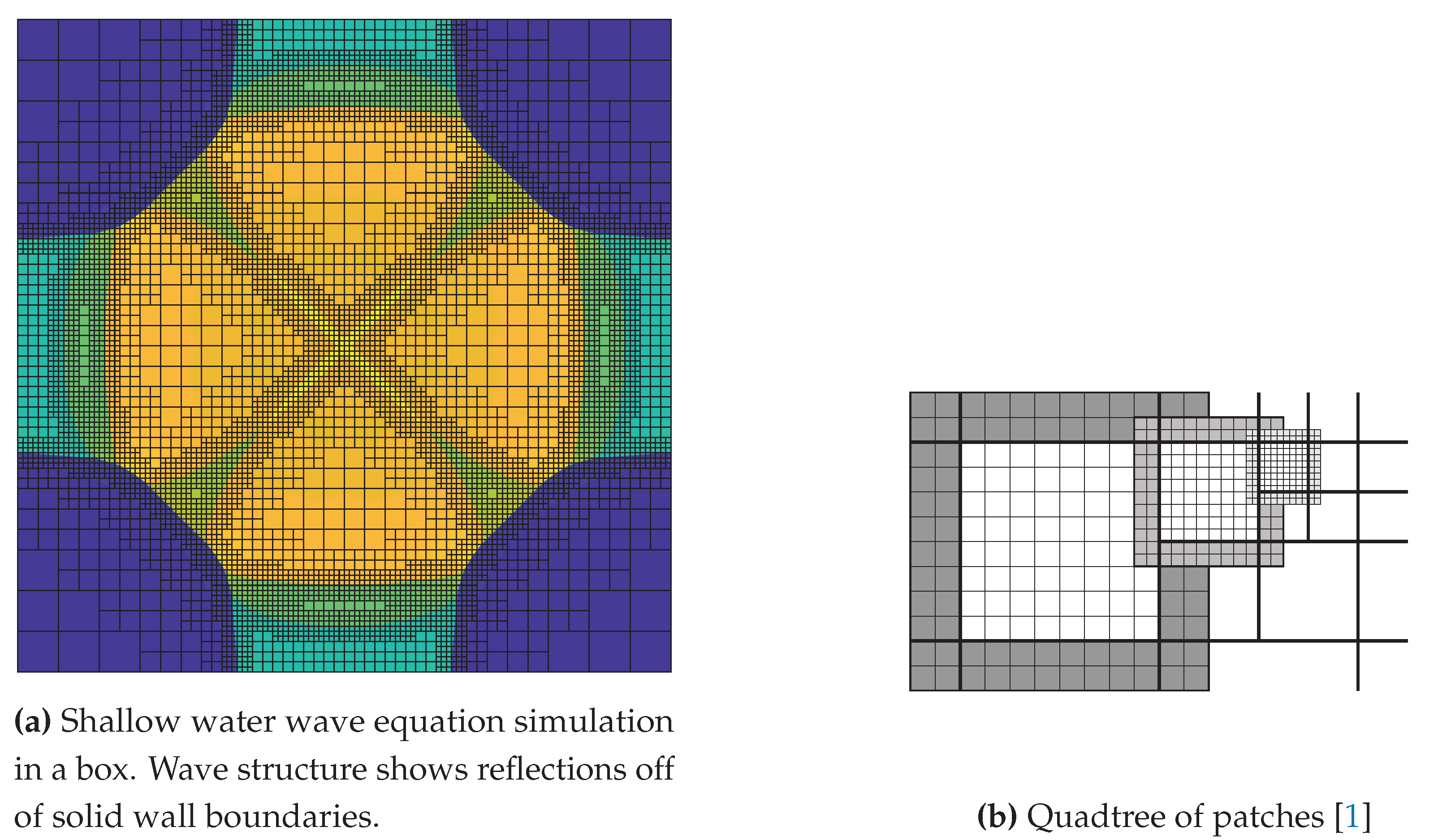
The multi-resolution grid hierarchy in ForestClaw is a composite structure of non-overlapping fixed-sized grids (e.g. ), each stored as a leaf in a quad or octree forest. This makes it easy to apply Cartesian mesh methods to problems with complex geometries like a cubed sphere and other non-regular regions.
Figure 1.
The left figure depicts an adaptively refined ForestClaw-simulated SWE solution on a Cartesian grid in the quadtree layout on a single block. The right figure depicts three adjacent adaptive levels, each with an simulation grid (with thick borders) and a layer of ghost cells. Quadrant boundaries are indicated by thick lines.
4.1. GeoFlood Refinement Criteria
A new AMR strategy based on flags imposed by different refinement criteria has been developed in the GeoFlood code. These include: 1). Water depth criteria, where refinement is permitted only in wet cell regions by imposing a flag on cells with water depths greater than a certain threshold value and the refinement level is determined by the water depth. 2). Bathymetry flag, used to force refinement in shallow regions where the flow changes rapidly such as near river banks or shorelines. 3). Velocity criteria, which assume that the magnitude of the water velocity in both and directions is greater than a certain threshold value. 4). Flood source flags, used to force refinement in regions containing the flood source, i.e., the dam in the case of a dam break. This allows the code to refine the flood source at high resolution to capture the flood details along the floodplain and allows the specification of regions to be refined to a given desired resolution by user-specified coordinates and minimum and maximum refinement levels. This criteria can also specify regions of less interest where refinement should be avoided 5). Flow-grades flag, where refinement is enforced to given levels for depths or velocities greater than user-defined thresholds. This enables the code to refine regions containing lakes, seas, or rivers in the floodplain at varying intermediate levels compared to the flowing material.
5. Benchmark Test Cases
We selected a series of benchmark scenarios, designed by the United Kingdom Environment Agency [
2], to evaluate the capabilities of GeoFlood within the context of flood risk management. This evaluation focused on the model’s precision in replicating flood progression and the extent of inundation across diverse physical landscapes and configurations. The performance of GeoFlood in these benchmark tests was evaluated by comparing results with those obtained from both HEC-RAS and GeoClaw under identical test conditions. These test cases have also been previously employed in the benchmarking of various other models, including HEC-RAS. For a more comprehensive overview of these benchmarking studies, see, for example, [
2,
5,
49].
5.1. Test Case 1: Filling of Floodplain Depressions
5.1.1. Problem Setup
We first examine GeoFlood results for a benchmark that entails the filling of floodplain depressions. This test is designed to evaluate GeoFlood’s predictive accuracy in determining the inundation extent and final depth of flooding over a long period of time under conditions of low-momentum flow across intricate topographical landscapes. The primary focus of this assessment is on the final distribution of the floodwaters, rather than their peak levels.
The computational domain of this test is a square with a side length of 2000 m.
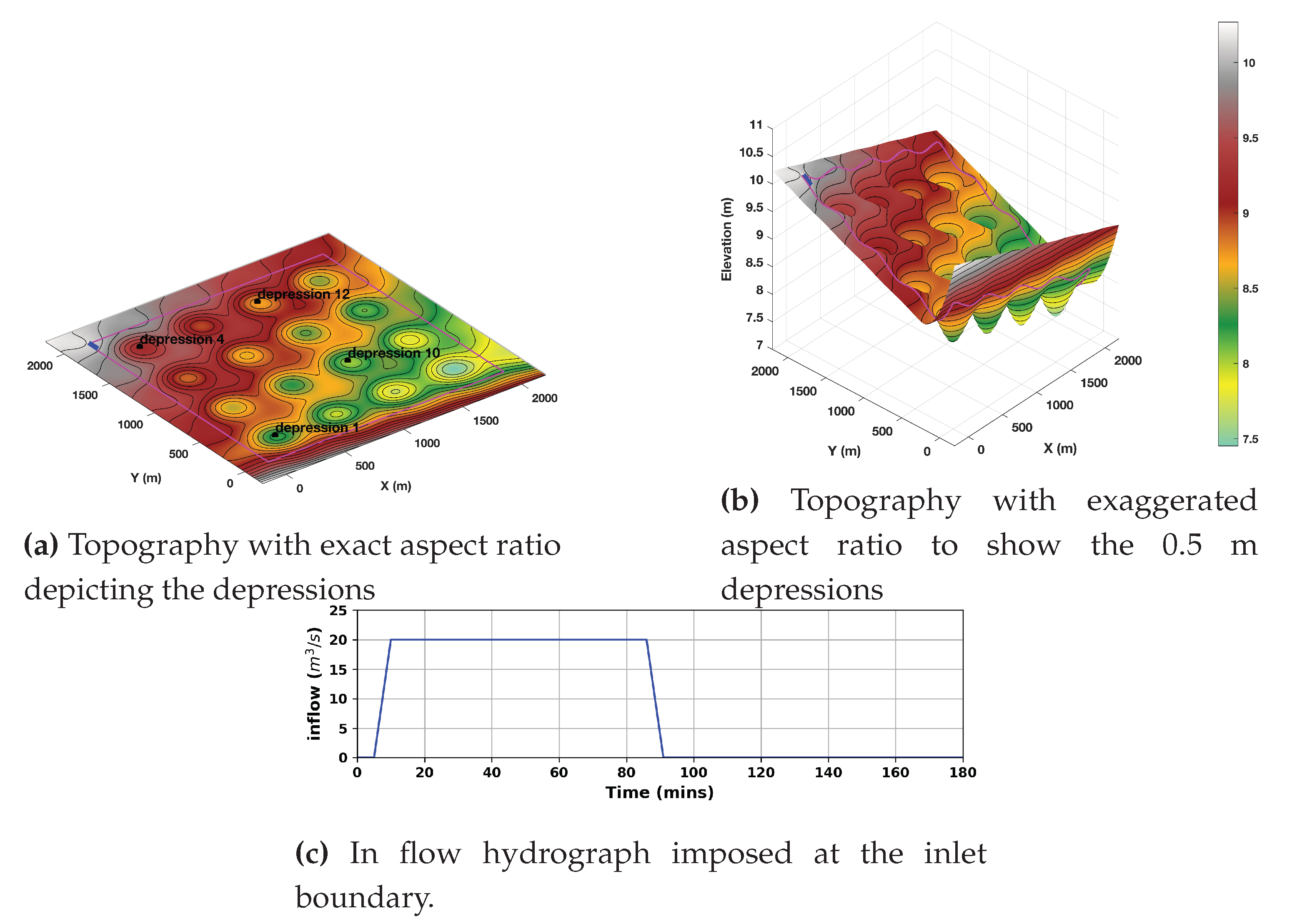
Figure 2 depicts a
matrix of
m deep depressions with smooth topographic transitions obtained by multiplying sinusoids in the north-to-south and west-to-east directions. The underlying average slope is
in the north-south direction and
in the west-east direction, with an elevation drop of about 2 m along the northwest-to-south diagonal. At the upstream boundary (northwest of the domain), an inlet hydrograph with a peak flow of 20m
3/s and a time base of approximately 85 minutes is imposed along a 100 m long line (blue thick line) that runs north to south, as shown in
Figure 2. We linearly interpolated this inlet hydrograph, divided by the channel width, at the simulation time steps to obtain the inflow momentum
. This value was used to set the momentum in ghost cell values at the channel along the left side of the computational grid.
To get the depth
in the ghost cells, we solve
where
,
and
were taken from the first interior grid cell. To avoid numerical difficulties, if
was non-zero, but less than the dry tolerance
, we set
before solving for
.
If , we filled ghost cells values at the channel edge by applying a wall boundary condition using interior values and .
If, after solving for
in (
10),
, the entropy satisfying Riemann solution was determined from a 2-shock wave rather than Riemann invariants. In those cases, we recomputed
by solving
Equations (
10) and (
12) were solved using the Newton Raphson method to determine the depth
in ghost cells. The Newton solver was initialized using an initial estimate
, where the constant
F is the Froude number, which we set to 0.5 for the Riemann invariant problem and to 1 for the two shock problem. All other boundaries were treated as solid wall boundaries, and the initial condition assumes a dry bed.
The problem is simulated for two days (48 hours) to achieve a final hydrostatic steady state. The following numerical configurations were used: a wet-dry threshold of 0.0001m, an adaptive time step with a CFL (Courant-Friedrichs-Lewy) ranging from to , and a Manning coefficient of .
5.1.2. Test Case 1: Simulation Results
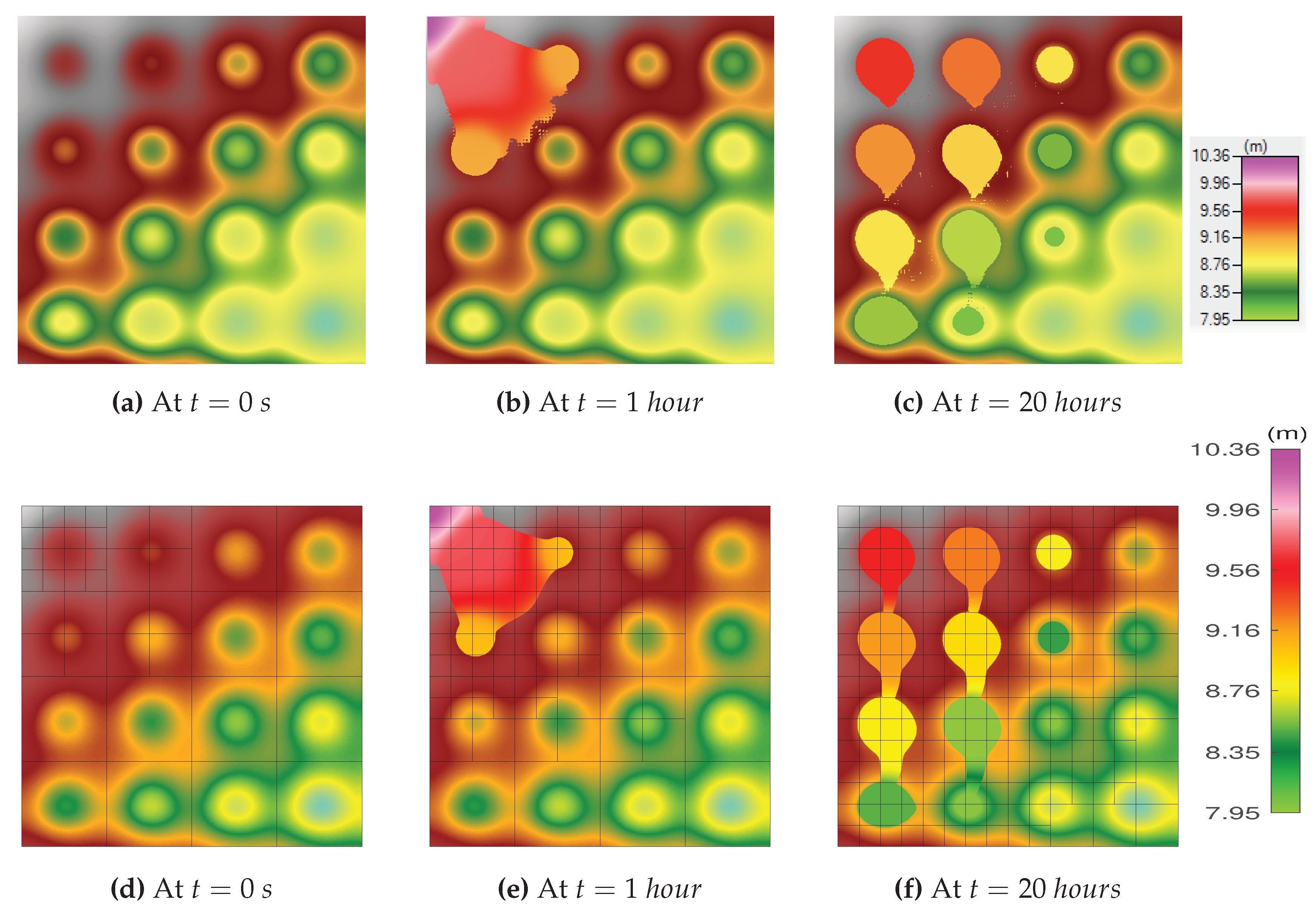
Figure 3,
Figure 3, and
Figure 3 show the adaptively refined solution simulated by GeoFlood at times
,
hours, and
hours, respectively, at mesh refinement levels: 0, 1, and 2, on a
grid of 4 level 0 blocks in each of the x- and y-directions, yielding a 10m grid resolution at level 0 and 2.5m at level 2. We compare the results with those from HEC-RAS on a uniform
grid of 10m resolution.
Figure 3 shows that during the influx, a transient water level peak was observed close to the inflow. Following the cessation of the inflow, each depression’s water level steadily dropped until it eventually reached the level of the lowest "sill" separating it from adjacent depressions, as shown in
Figure 3 after 20 hours.
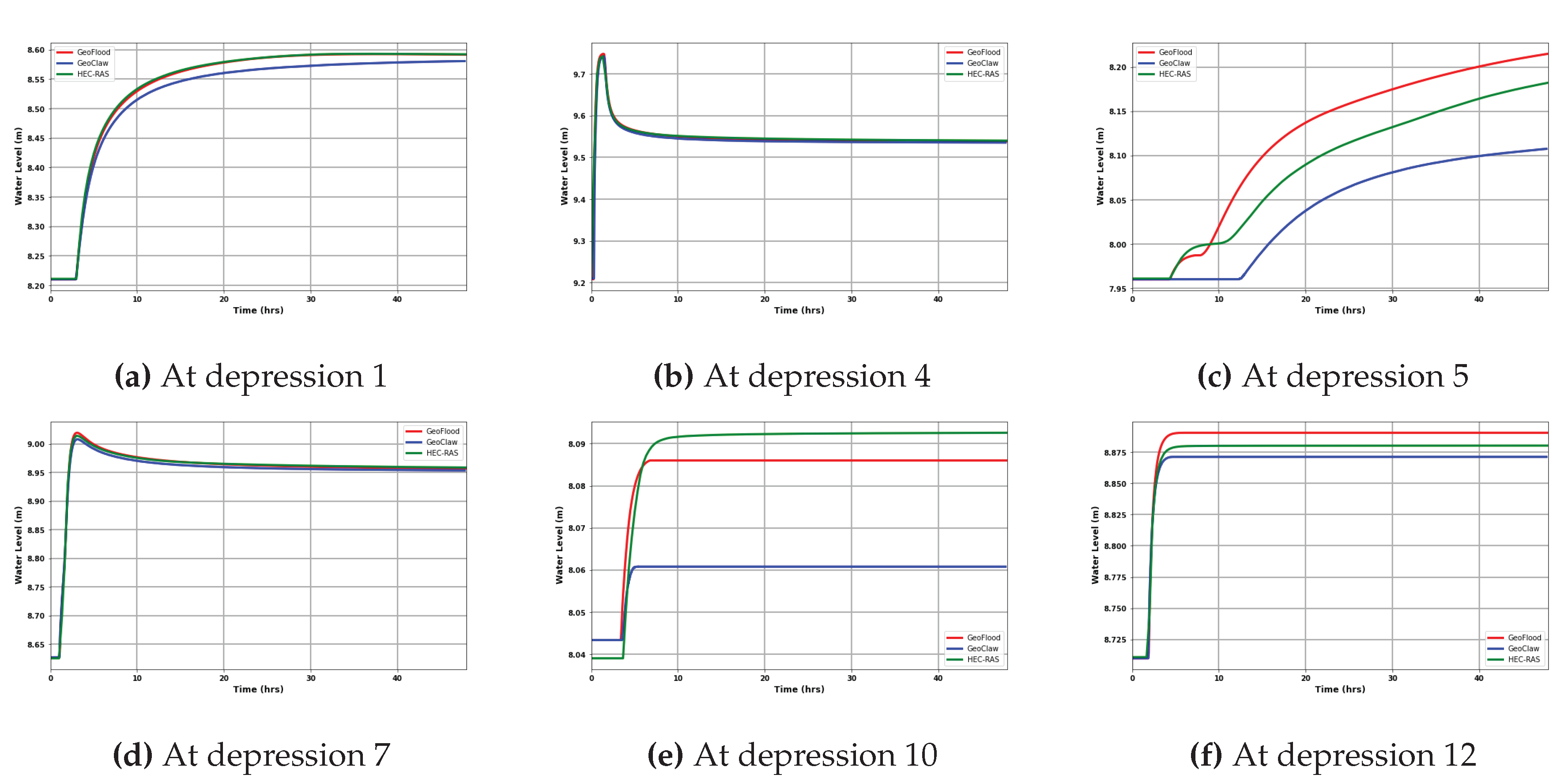
Figure 4 depicts the water surface elevation time series at six depressions: 1, 4, 5, 7, 10, and 12. Overall, GeoFlood generated results that were comparable to those of HEC-RAS and GeoClaw and predicted the flood extent at all depressions. On the other hand, different flood arrival times and initial flood amplitudes were observed at depressions 5 and 10 for all the models, indicating a sensitivity that we attribute to the extremely shallow flow between the depressions over the thresholds and relatively slight differences in wave dynamics. We attribute the slight difference between the water elevations observed in the depressions 10 and 12 to the shallower depths reached and the bowl-shaped topography at these depressions.
5.2. Test Case 2: Speed of Flood Propagation Over an Extended Floodplain
5.2.1. Problem Setup
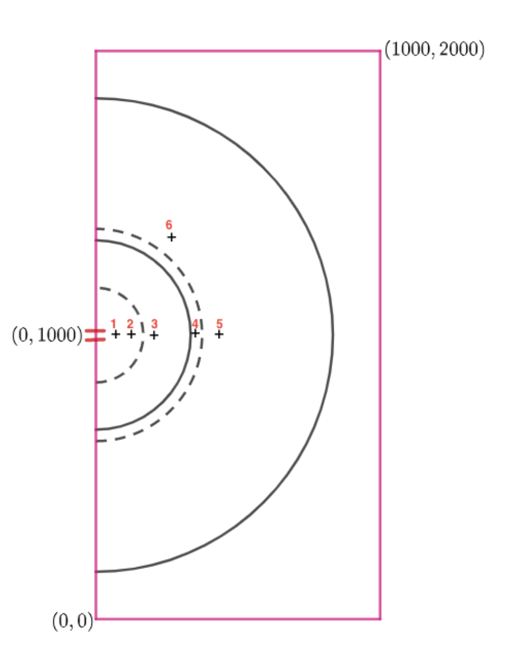
In this second test, our goal is to see how well GeoFlood can simulate flood wave propagation speed and predict changing velocities and depth at the leading edge of an advancing flood. This applies to both river and coastal flooding caused by deteriorated embankments. The computational domain of this test is a rectangular domain with side lengths of 1000 m and widths of 2000 m. The elevation of the bed shown in
Figure 5 is a uniform 0 elevation. As shown in
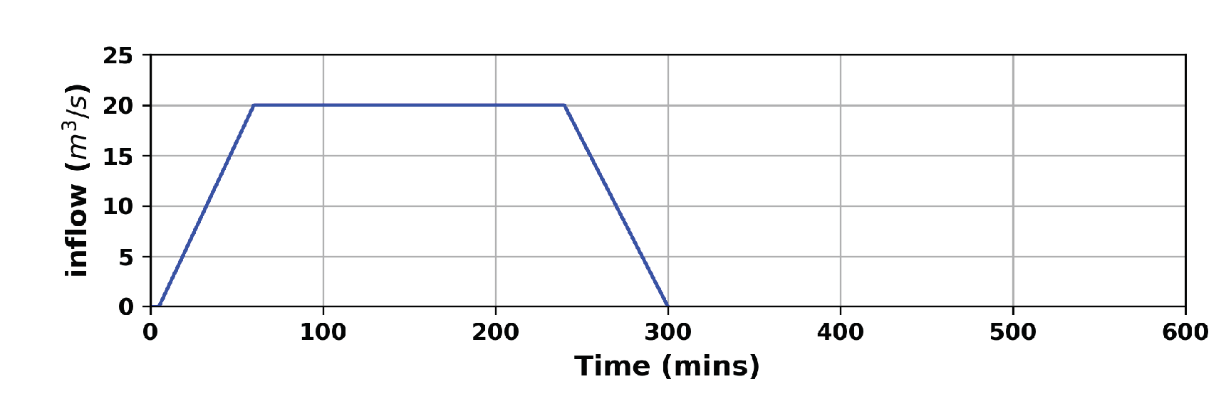
Figure 5, the inflow hydrograph is imposed in the middle of the left boundary, along a line of 20 m long that runs from north to south. This inflow hydrograph starts at zero and rises linearly to a peak value of 20 m
3/s during the first 60 minutes of the experiment. It remains constant for the next 180 minutes before dropping linearly to zero for the final 60 minutes. All other boundaries are closed, and the initial condition considered is a dry bed.
The spatial domain was discretized into
cells with a uniform grid spacing of 5 m in both the
and
directions. The following numerical configurations were used: a wet dry threshold of
m, an adaptive time step with a CFL ranging from
to
, a final time of 6 hours, and a Manning coefficient of
. The inflow hydrograph boundary condition was implemented as described in
Section 5.1.1.
5.2.2. Test Case 2: Simulation Results
In
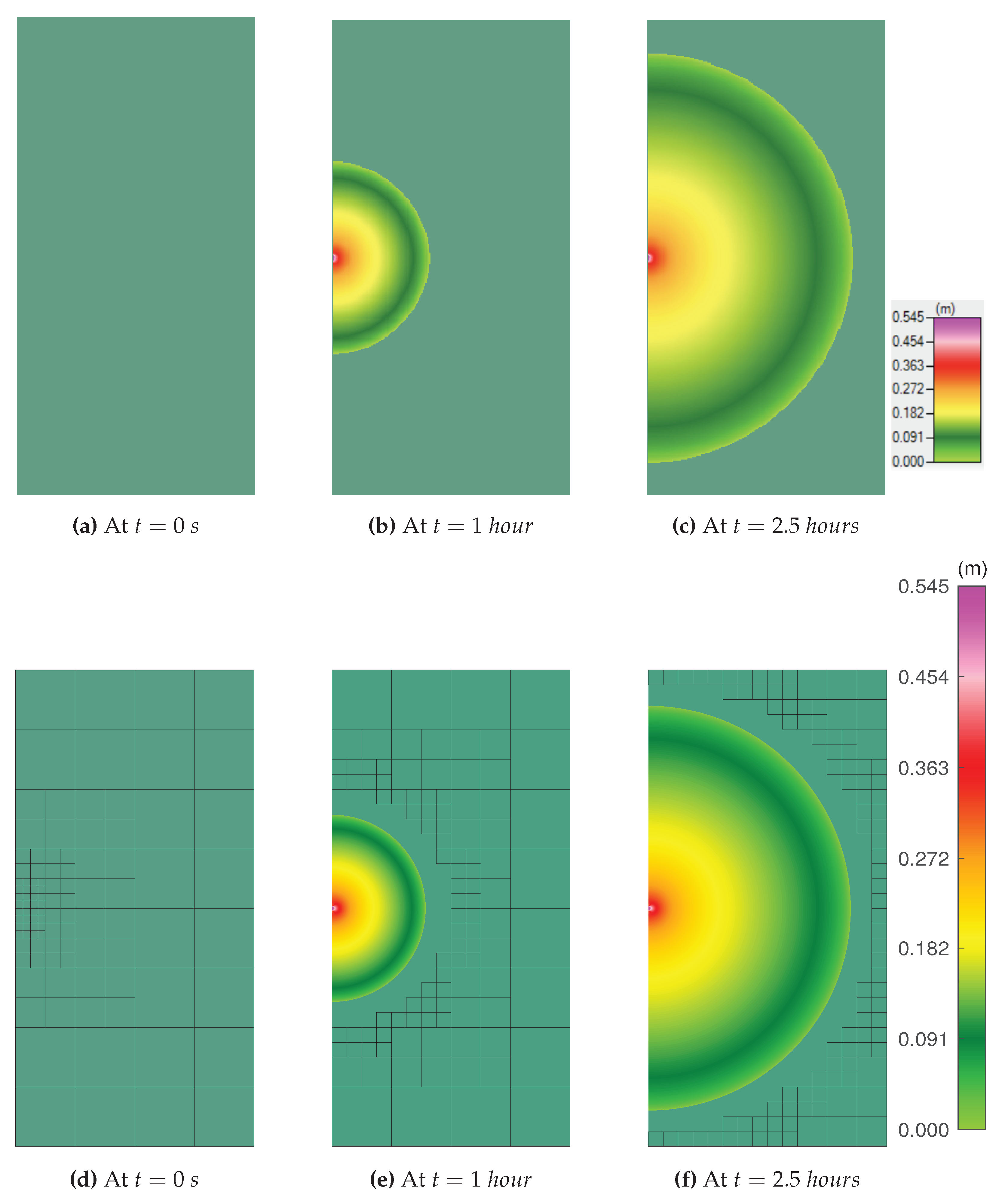
Figure 7, the embankment was refined to the highest level available to accurately capture the extent of the flood along the flood plain. The model comparison shows that GeoFlood simulated the celerity of the propagation of the flood wave along the dry floodplain similarly to HEC-RAS. We attribute the difference in the speed of the flood front to differences in the implementation of boundary conditions and HEC-RAS’s treatment of the source term, which differs significantly from that of GeoFlood and GeoClaw.
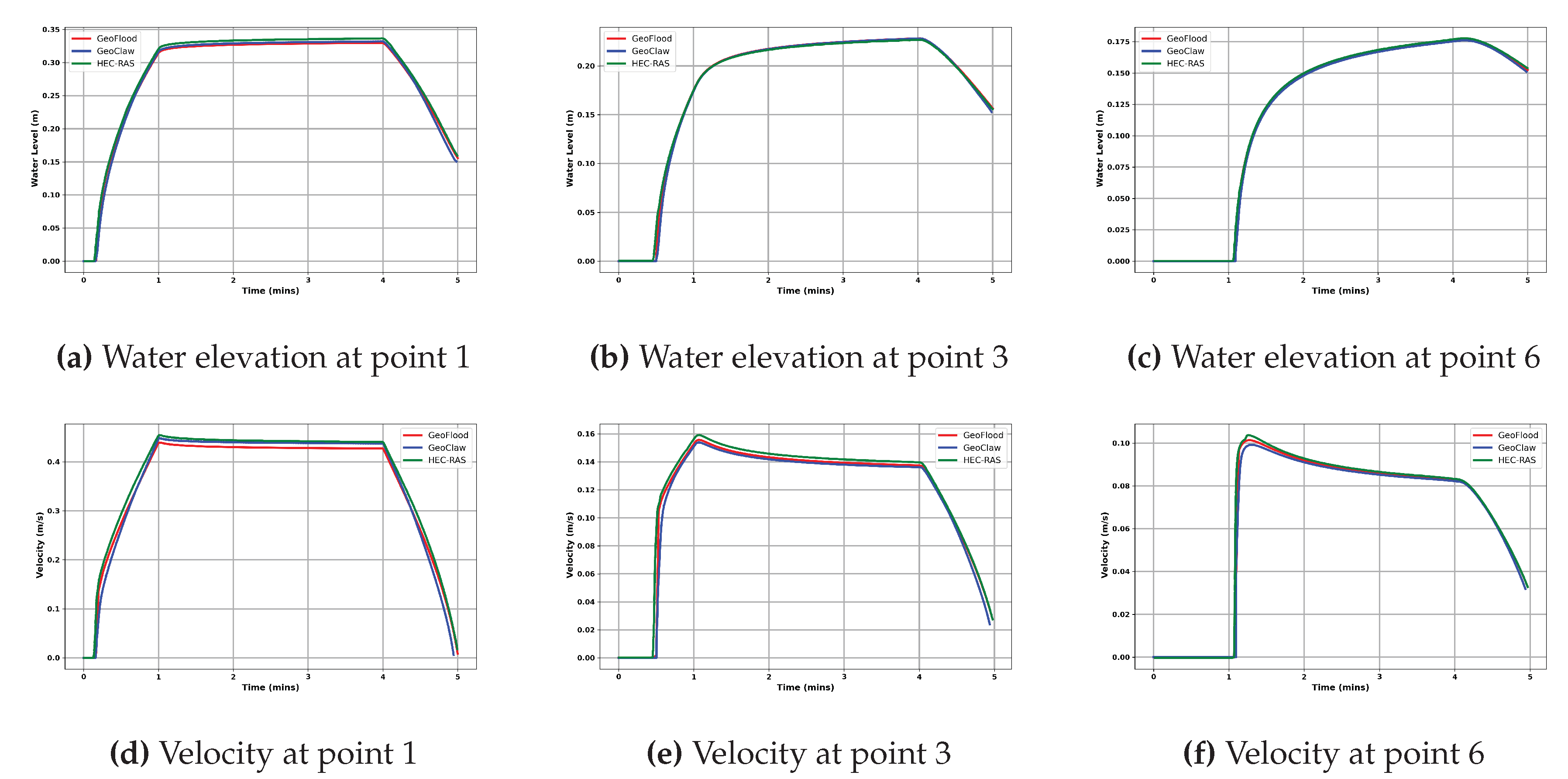
Figure 8 compares GeoFlood simulations with GeoClaw and HEC-RAS temporal evolution of elevation and velocity of the water surface at several control points in the flood plain. These simulations represent GeoFlood’s capabilities to predict the depths and transient velocities at the leading edge of the flood front. Overall, GeoFlood results are in agreement with GeoClaw and HEC-RAS results.
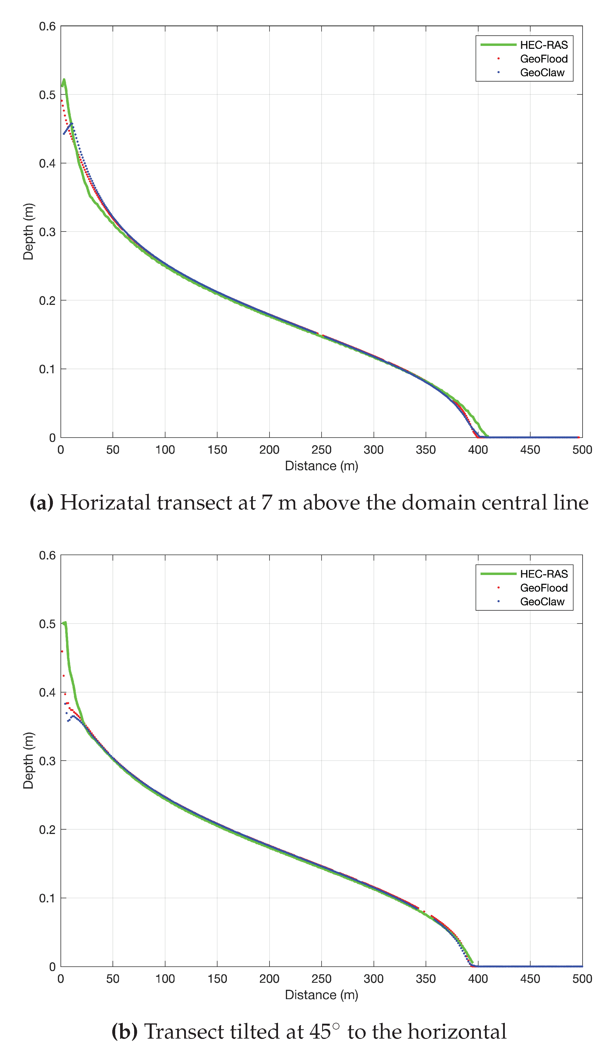
Figure 9 represents the cross-section of depths at 7 m above the horizontal central line through the domain at time
hour for HEC-RAS, GeoFlood, and GeoClaw models. The results show that these three models have consistent results along that line. We choose a horizontal line 7 m above the central horizontal line within the domain due to the unique characteristics of the block-structured adaptive mesh refinement employed in the GeoFlood model, which prevents us from obtaining data at the interfaces of adjacent grid cells. The observed disparities in the initiation points of the depth profiles for each model are likely due to the differing methodologies employed in mesh management and the adaptive time-stepping algorithms, which are particularly sensitive to the initial dry state conditions. Except for the onset phase, GeoFlood and GeoClaw present identical results along the transect, corroborating the expectation due to the application of identical Riemann solvers in both models.
In
Figure 9, a cross-section of depths is displayed, tilted at
to horizontal starting from the point
at a height of 7 meters above the horizontal centerline and extending to the upper-left corner point
. The results from this transect also exhibit nearly identical outcomes as the other three models, demonstrating that all the models predict the same surface flow.
5.3. Test Case 3: Dam Break
5.3.1. Problem Setup
For the third benchmark test, our objective was to verify GeoFlood’s ability to accurately simulate transcritical flows, hydraulic jumps, and wakes behind obstacles. This test case involves the rupture of a dam in a laboratory scale model and is presented in [
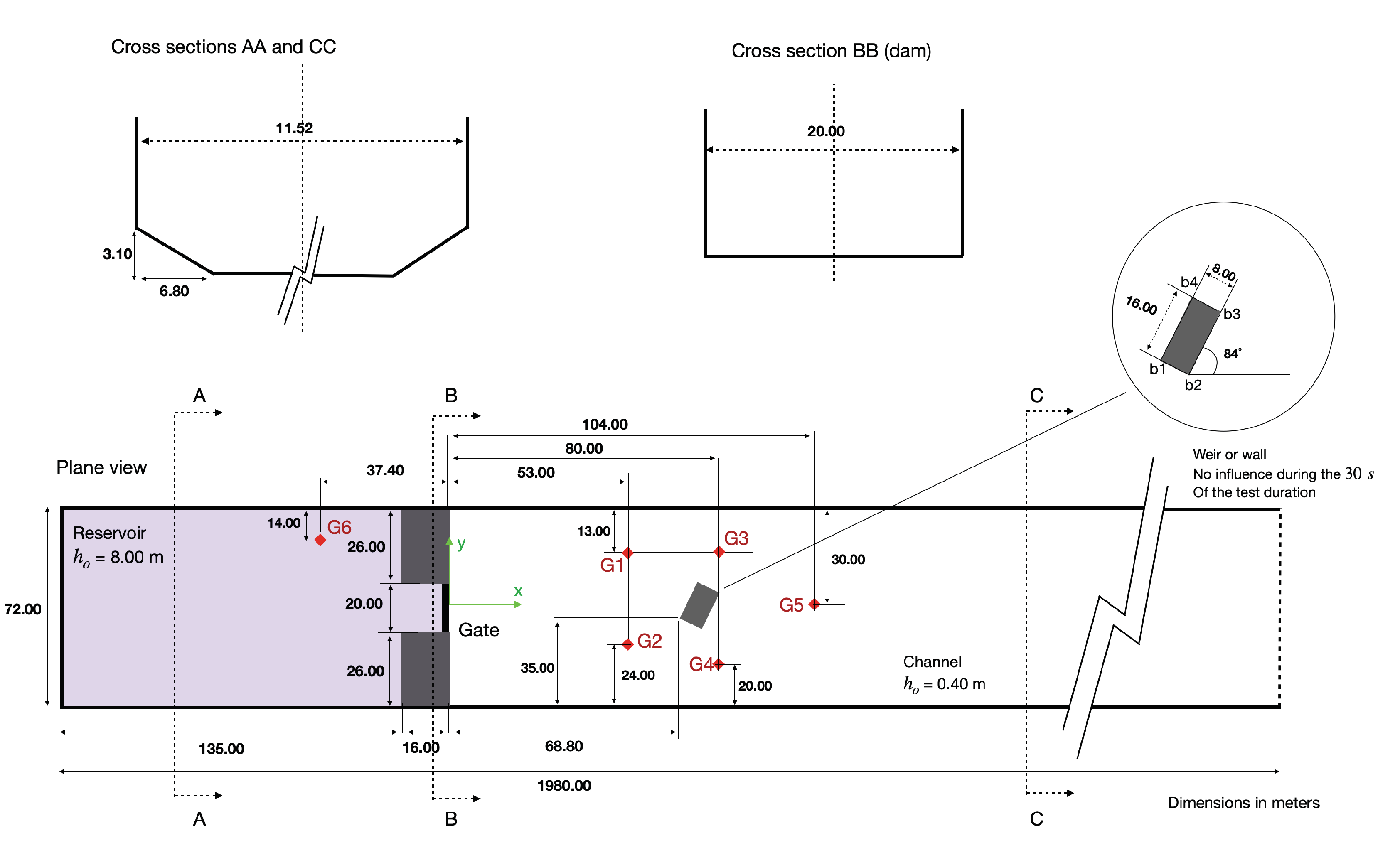
50]. Physical parameters have been scaled by 20 times relative to the experimental set-up in order to replicate the scale of a real-world dam break scenario. In the experiment, a dam-break wave was generated by the nearly instantaneous opening of the gate at the end of the reservoir. The wave then collided with an oblique rectangular obstacle positioned downstream of the dam, producing a hydraulic jump just upstream of the obstacle and a wake zone downstream as shown in
Figure 10 and
Figure 11.
Our computational domain was 1980 m long and 72 m wide. The simulation was run for 30 minutes. The following numerical configurations were used: a wet-dry threshold of
, an adaptive time step with a CFL ranging from
to
, and a Manning coefficient of
. The geometry and dimensions for the dam break test are shown in
Figure 10.
5.3.2. Test Case 3: Simulation Results
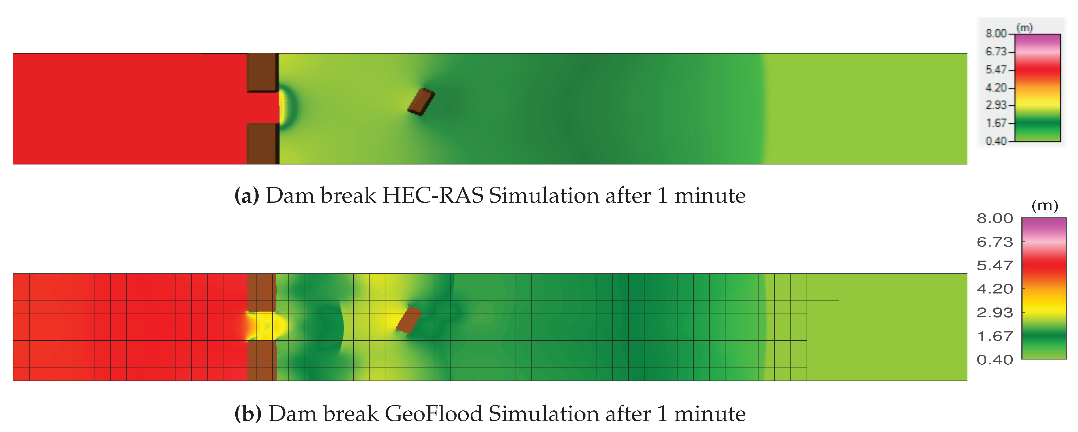
The spatial evolution of the flow downstream after 1 minute is depicted in
Figure 11 and
Figure 11 for HEC-RAS and GeoFlood respectively. As seen in the figures, both models produce a downstream water level that remains at
m. The HEC-RAS solution was computed on a uniform
grid, while the GeoFlood solution utilized an adaptive
grid with max level = 3, min level = 1, and
block arrangement in the x and y directions, respectively.
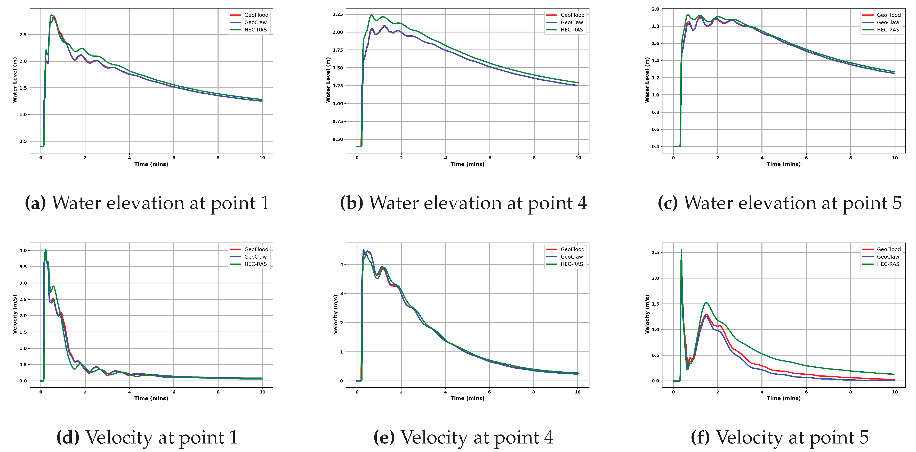
Figure 12 shows the temporal variation of the surface water elevation and velocity at various control points of GeoFlood compared against the GeoClaw and the HEC-RAS models. Results demonstrate generally consistent predictions between the three models, even though some degree of oscillatory behavior is observed in the high momentum regions downstream of the gate.
6. Malpasset Dam Break Simulations
For our final test case, we assess GeoFlood’s ability to replicate a historical dam break and overland flood event. The availability of field data and numerical results provide a means for verification and validation of GeoFlood for real-world problems [e.g., [
3,
51].
6.1. Historical Background
The Malpasset Dam is situated approximately 12 km upstream from the town of Frejus, France. This thin-arch dam was constructed in a narrow gorge above the Reyran River valley in order to impound a reservoir with a storage capacity of
. Upon reaching reservoir capacity, the dam failed suddenly and catastrophically on December 2
nd, 1959 at
hours (generating an acoustic shock wave observed in Frejus, suggesting a nearly instantaneous failure). The dam had a maximum height of
m and a crest span of 223 m. Only remnants of the dam’s arch remained after the failure, with significant erosion of the adjacent rock bank. Subsequent investigations suggest that the arch dislodged from its base leading to a rapid sequential collapse [
10].
The catastrophic breach led to a rapid flood wave that descended through the channelized ravine, eventually inundating the wide floodplain adjacent to the Mediterranean and surrounding Frejus. The event resulted in 433 fatalities and significant infrastructure damages, including the obliteration of a
km section of freeway and an adjoining bridge, and extensive flooding of Frejus. The downstream displacement of massive blocks indicated the power of the flood. The flood waves rose to
m above the original riverbed. A complete description of this event can be found in [
52].
6.2. Topography
Due to the dramatic changes in the topography after the accident, historical maps (carte IGN map of Saint-Tropez , dated 1931) were used to digitize the valley bottom elevation in order to assess topographic changes. The streambed thalweg downstream of the dam traverses a pronounced depression followed by two steep and narrow bends. The drainage channel then widens beyond the confluence of multiple tributaries with the Reyran River. It becomes narrower again further downstream and has several more large bends before eventually reaching the low-lying broad alluvial fan in the Reyran River valley surrounding Frejus.
Our study’s overall dimensions are 17500 m
m. The valley floor elevation ranges from
m below sea level (the sea is included in the calculation) to
m above sea level, the latter being the reservoir’s estimated initial free surface elevation. This initial free surface has a
cm of uncertainty, which is negligible given the total volume of water released. The topography for the GeoFlood simulations originated from a benchmarking exercise in 1999, sponsored by CADAM (Concerted Action on Dam-break Modelling) project, a European research group [
27] which included a set of 13541 irregularly spaced points of known coordinates used in the numerical domain description.
6.3. Initial and Boundary Conditions
The sea level and the initial reservoir level are assumed to be constant and are set at 0 and 100 m above sea level, respectively. Although the outlet gate near the bottom of the dam was open during the event, we neglected pre-event streamflow in the channel—the bottom was considered dry. The actual pre-event streamflow discharge is unknown, but we assumed that it was relatively negligible. Since the value of the inlet discharge upstream of the reservoir is unknown, an imposed discharge constant of zero was used. The sea level remained constant and equal to zero. We assume an instantaneous dam failure.
6.4. Simulation Results
In our simulations, we used a Manning coefficient of , as recommended by the CADAM for their modeling exercise. The GeoFlood simulation runs were done on a GHz Quad-Core Intel Core processor with 16 GB of RAM required approximately 30 minutes of wall clock time to complete the entire scenario, a total simulated time of 4000 seconds. Our simulation utilized a computational grid measuring 32 m m, with the levels of grid refinement ranging from 1 to 4. The model operated with an initial time step of 1 second, adhering to a CFL number set at .
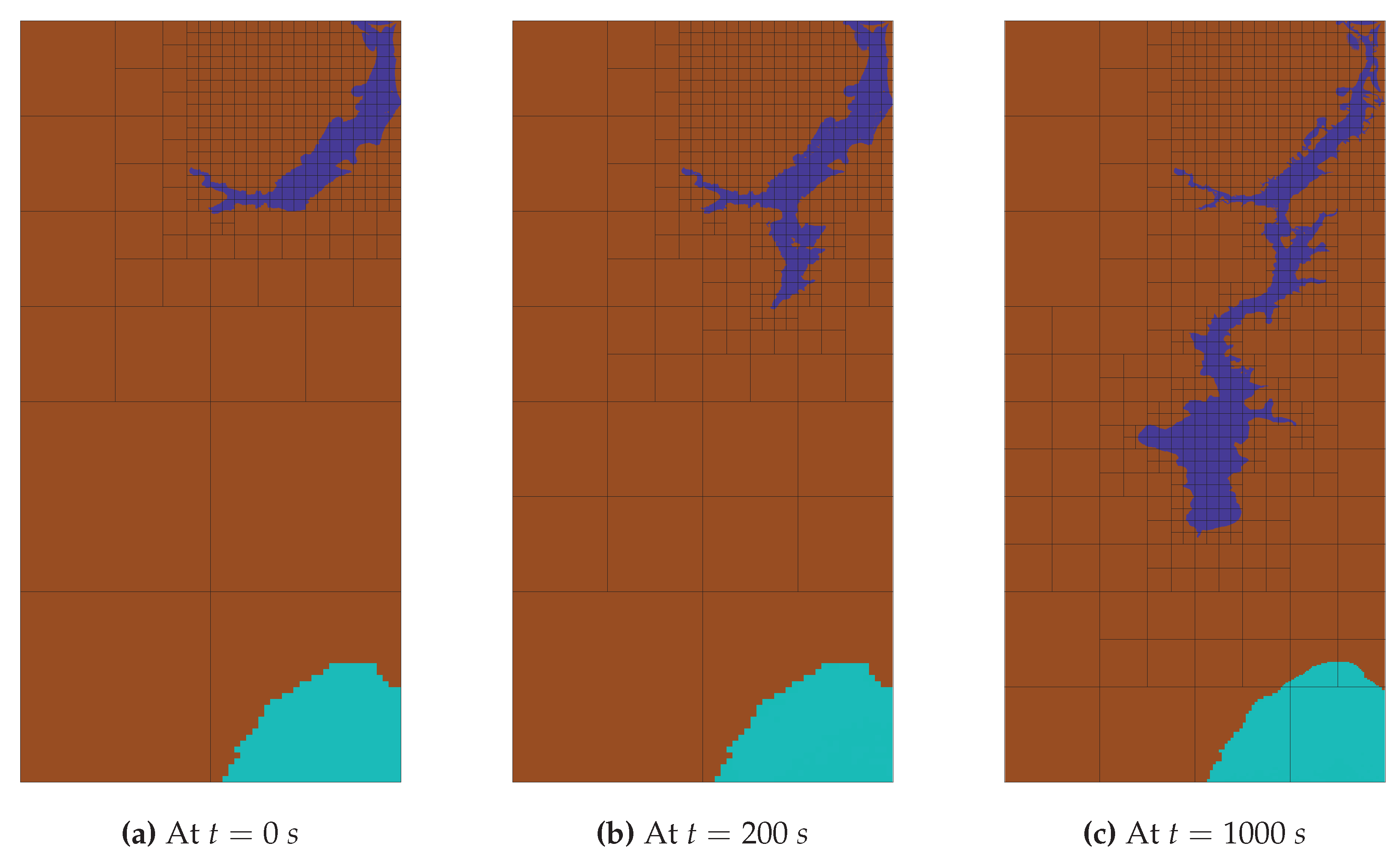
The novel adaptive mesh refinement flags, designed considering multiple criteria such as water depth, bathymetry, velocity, topographical features, and the origin of the flood, facilitated precise refinement in particular areas of the simulation domain. This approach accurately represented the flood’s scope and intricate details in the areas surrounding the floodplain during the dam break, as demonstrated in
Figure 14 and
Figure 15. Consequently, this led to the generation of simulations with high-resolution mesh adaptations in the vicinity of the dam and floodplain, as depicted in
Figure 14. Furthermore, this approach yielded strong correlations between the simulation outcomes, field observations, and numerical results from various models, as evidenced in
Figure 13 and
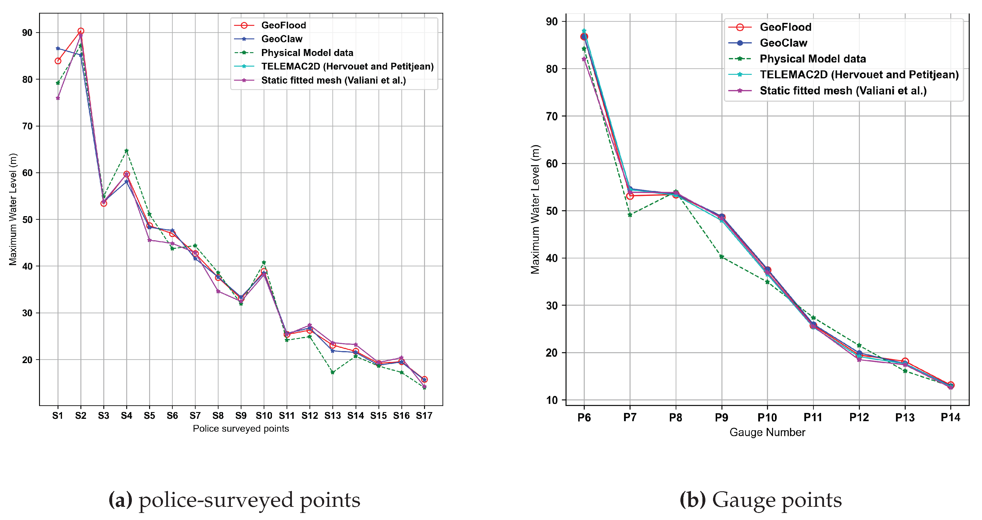
Figure 13. In these figures, the comparison is drawn between the GeoFlood simulated results at the 17 field-surveyed and 9 gauge locations against the field and experimental data, with the numerical results from GeoClaw from George [
3], and other flood modeling approaches.
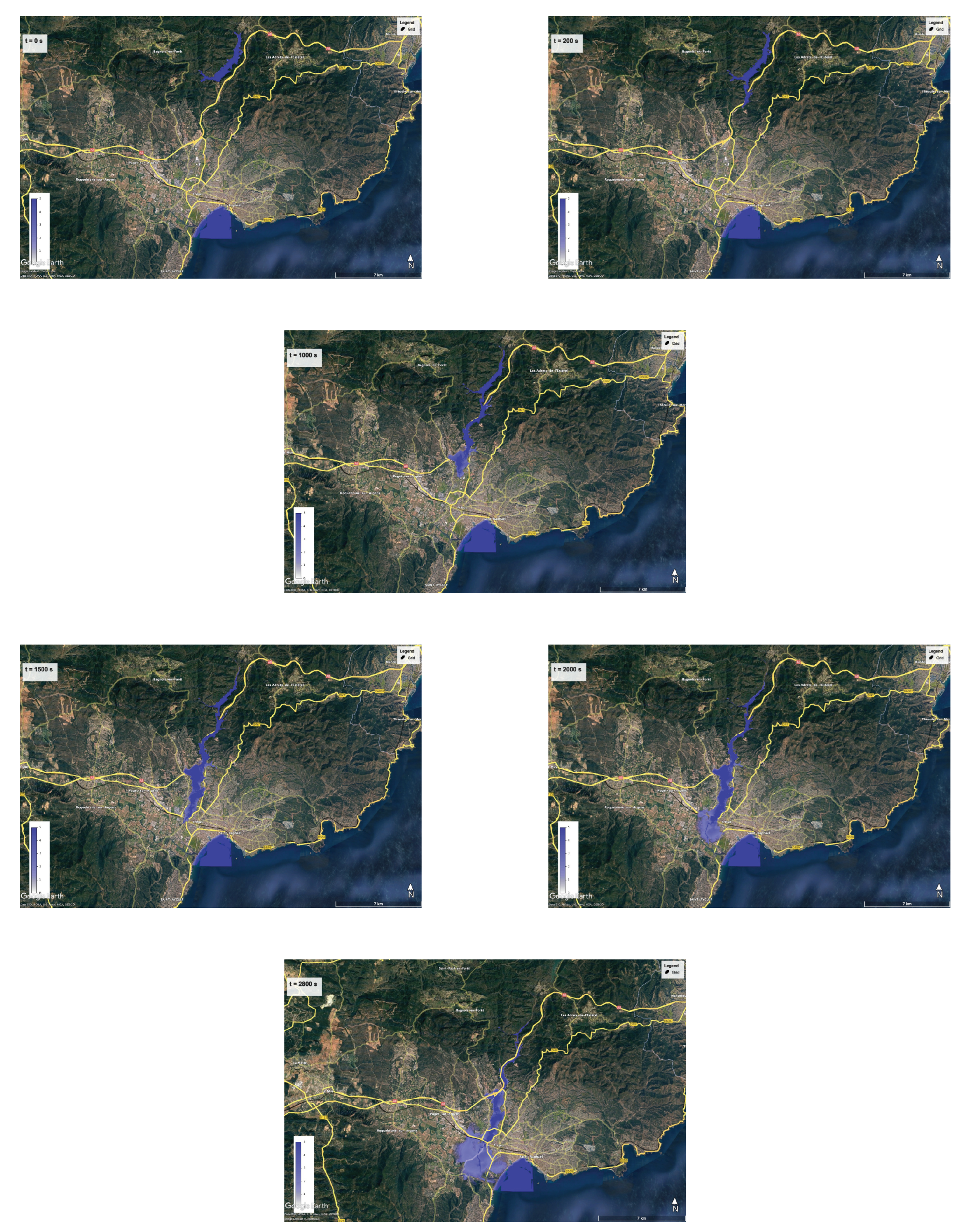
Innovative procedures incorporated into GeoFlood for projecting simulation frames within a non-latitude-longitude coordinate framework onto Google Earth are depicted in
Figure 15. These outcomes validate the model’s proficiency in replicating the flood scenario across intricate topography, effectively capturing both the temporal progression and spatial expansion of the flood’s extent.
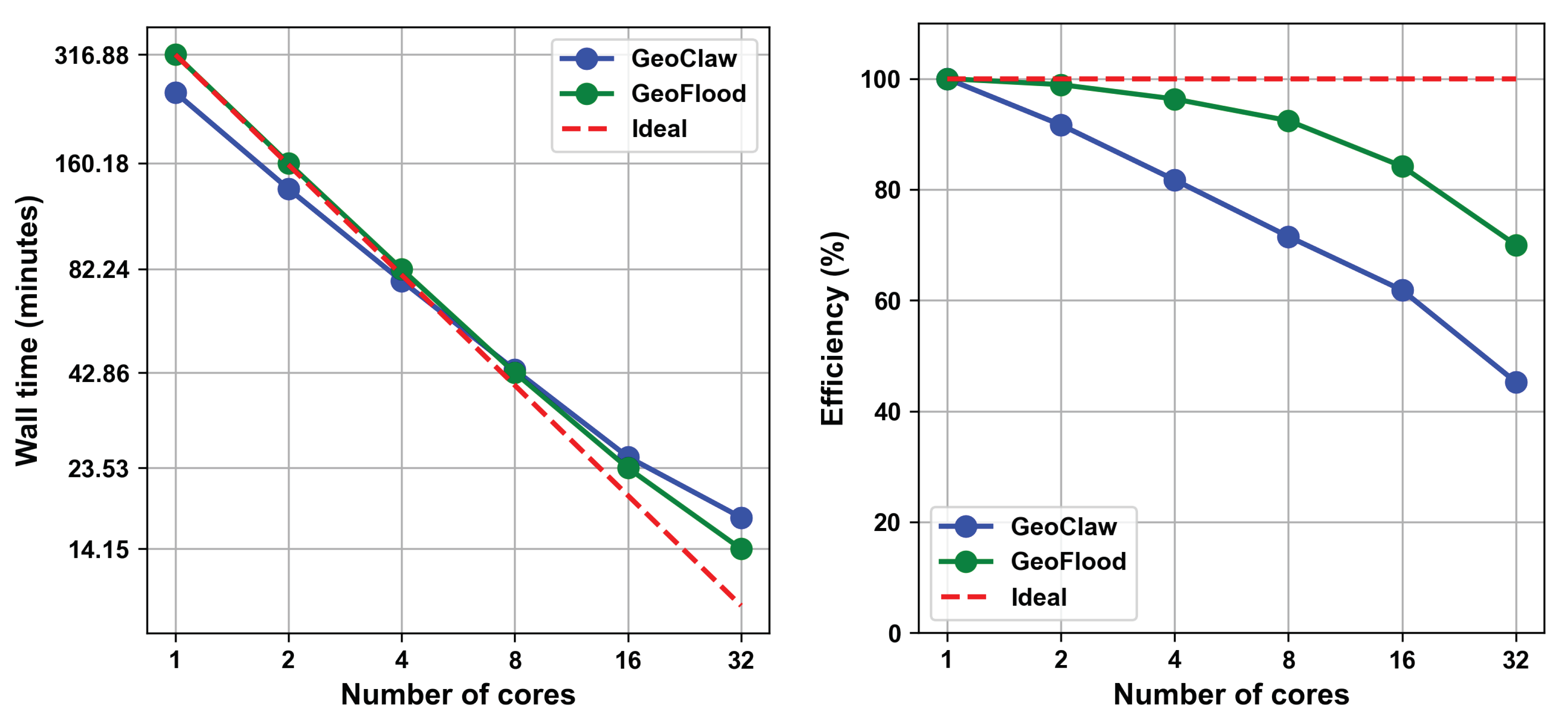
The incorporation of multi-block-based adaptive mesh refinement, as facilitated by ForestClaw, alongside refinement flags, the creation of novel routines for topographical data and input handling, as well as the strategic integration of function linkage between code libraries, collectively contributed to GeoFlood’s efficient performance. Particularly evident is the parallel efficiency and computational time at higher processor counts 8, 16, and 32 as depicted in
Figure 16. The use of ForestClaw also resulted in improved load distribution across nodes and a reduction in idle time per node.
These findings, presented in
Figure 16, were derived from tests conducted on a Linux-based supercomputer (Borah) equipped with 181 CPU nodes, each with 48 cores and 192 GB of memory. Experiments involving various numbers of nodes and cores per node were conducted to assess the scalability and efficiency of each code. The results, as shown in
Figure 16, reveal that GeoFlood outperforms GeoClaw in efficiency across all tested runs. This is likely due to the fact that the dynamic regridding process in GeoFlood is fully parallelized through the mesh management libraries ForestClaw and p4est. This is in contrast to GeoClaw, which can only carry out the dynamic regridding in serial.
The comparative analysis presented in
Figure 16 reveals that in the initial phase involving up to three processors (specifically,
, and 4), GeoClaw demonstrates a reduced wall time compared to GeoFlood. However, beyond this point, GeoFlood surpasses GeoClaw in performance.
7. Conclusions
The development of the GeoFlood model has been accomplished with a focus on accurately simulating flooding in intricate landscapes. Its performance was rigorously tested and confirmed through three distinct benchmark challenges. Benchmark simulation results were compared with those from the HEC-RAS and GeoClaw models. GeoFlood results on the Malpasset dam break incident were corroborated using field data, laboratory scale-model data, and numerical results from prior studies. These evaluations revealed GeoFlood’s capability to effectively forecast the trajectory of flood waves, showing strong agreement with actual recorded events. A notable aspect of GeoFlood is its scalability, which qualifies it for application in modeling large-scale flood scenarios. The insights gained from this research hold considerable value for the advancement of flood risk management strategies and the refinement of flood hazard mapping techniques.
Author Contributions
Brian Kyanjo drafted the manuscript, set up and carried out the simulations, and designed the code under the supervision of Donna Calhoun and David L George. The authors read and approved the final manuscript.
Data Availability Statement
Acknowledgments
The authors would like to extend there gratitude to all contributors and developers of ForestClaw, GeoClaw, and p4est (Carsten Burstedde) for making their codes publicly available, Yu-hsuan (Melody) Shih the initial implementer of GeoClaw solver in ForestClaw, and Boise State University for providing computational resources for this study. The authors also acknowledge the financial support of the DARPA AtmosSense program, NASA ROSES Earth Surface and Interior Program, and NSF-DMS award #1819257.
Conflicts of Interest
The authors declare no competing interests present
References
- Calhoun, D.; Burstedde, C. ForestClaw: A parallel algorithm for patch-based adaptive mesh refinement on a forest of quadtrees. arXiv preprint, 2017; arXiv:1703.03116. [Google Scholar]
- Neelz, S.; Pender, G. Benchmarking the latest generation of 2D Hydraulic Modelling Packages. Technical report, Environment Agency: Bristol, UK, 2013.
- George, D. Adaptive finite volume methods with well-balanced Riemann solvers for modeling floods in rugged terrain: Application to the Malpasset dam-break flood (France, 1959). Int. J. Numer. Methods Fluids 2011, 66, 1000–1018. [Google Scholar] [CrossRef]
- Clawpack Development Team. Clawpack software, 2020. Version 5.7.1. [CrossRef]
- Brunner, G. Benchmarking of the HEC-RAS two-dimensional hydraulic modeling capabilities. Technical report, US Army Corps of Engineers: Davis, CA, USA, 2018.
- Luino, F.; TrebÒ, P. The Malpasset dam (France) fifty years after the failure of December 2, 1959 and references to similar Italian cases. Geoing. Ambient. e Mineraria 2010, 129, 53–80. [Google Scholar]
- Johnson, G.P.; Holmes, R.R.; Waite, L.A. The Great Flood of 1993 on the Upper Mississippi River—10 years later, 2004.
- Blumhardt, M. Colorado’s devastating 2013 Flood: A look back 9 years later, 2022.
- Filkins, D. A bigger problem than ISIS?, 2016.
- Valiani, A.; Caleffi, V.; Zanni, A. Case study: Malpasset dam-break simulation using a two-dimensional finite volume method. J. Hydraul. Eng. 2002, 128, 460–472. [Google Scholar] [CrossRef]
- Kirstetter, G.; Delestre, O.; Lagrée, P.Y.; Popinet, S.; Josserand, C. B-flood 1.0: an open-source Saint-Venant model for flash-flood simulation using adaptive refinement. Geosci. Model Dev. 2021, 14, 7117–7132. [Google Scholar] [CrossRef]
- Yu, H.L.; Chang, T.J. A hybrid shallow water solver for overland flow modelling in rural and urban areas. J. Hydrol. 2021, 598, 126262. [Google Scholar] [CrossRef]
- Coulibaly, G.; Leye, B.; Tazen, F.; Mounirou, L.A.; Karambiri, H. Urban Flood Modeling Using 2D Shallow-Water Equations in Ouagadougou, Burkina Faso. Water 2020, 12. [Google Scholar] [CrossRef]
- Shamkhalchian, A.; de Almeida, G.A.M. Effects of reconstruction of variables on the accuracy and computational performance of upscaling solutions of the shallow water equations. J. Hydraul. Res. 2023, 61, 409–421. [Google Scholar] [CrossRef]
- Rousseau, M.; Cerdan, O.; Delestre, O.; Dupros, F.; James, F.; Cordier, S. Overland Flow Modeling with the Shallow Water Equations Using a Well-Balanced Numerical Scheme: Better Predictions or Just More Complexity. J. Hydrol. Eng. 2015, 20, 04015012. [Google Scholar] [CrossRef]
- George, D.L. Augmented Riemann solvers for the shallow water equations over variable topography with steady states and inundation. J. Comput. Phys. 2008, 227, 3089–3113. [Google Scholar] [CrossRef]
- George, D.L. Finite volume methods and adaptive refinement for tsunami propagation and inundation; University of Washington, 2006.
- Berger, M.J.; George, D.L.; LeVeque, R.J.; Mandli, K.T. The GeoClaw software for depth-averaged flows with adaptive refinement. Adv. Water Resour. 2011, 34, 1195–1206. [Google Scholar] [CrossRef]
- Mandli, K.T. A numerical method for the two layer shallow water equations with dry states. Ocean Model. 2013, 72, 80–91. [Google Scholar] [CrossRef]
- LeVeque, R.J. Finite volume methods for hyperbolic problems; Vol. 31, Cambridge university press, 2002.
- Berger, M.J.; Oliger, J. Adaptive mesh refinement for hyperbolic partial differential equations. J. Comput. Phys. 1984, 53, 484–512. [Google Scholar] [CrossRef]
- Berger, M.J.; Colella, P. Local adaptive mesh refinement for shock hydrodynamics. J. Comput. Phys. 1989, 82, 64–84. [Google Scholar] [CrossRef]
- LeVeque, R.J.; George, D.L.; Berger, M.J. Tsunami modelling with adaptively refined finite volume methods. Acta Numer. 2011, 20, 211–289. [Google Scholar] [CrossRef]
- Mandli, K.T.; Ahmadia, A.J.; Berger, M.; Calhoun, D.; George, D.L.; Hadjimichael, Y.; Ketcheson, D.I.; Lemoine, G.I.; LeVeque, R.J. Clawpack: building an open source ecosystem for solving hyperbolic PDEs. Peer J Computer Science 2016, 2, e68. [Google Scholar] [CrossRef]
- Burstedde, C.; Wilcox, L.C.; Ghattas, O. p4est: Scalable Algorithms for Parallel Adaptive Mesh Refinement on Forests of Octrees. SIAM J. Sci. Comput. 2011, 33, 1103–1133. [Google Scholar] [CrossRef]
- Kyanjo, B. GeoFlood wiki. Git repository, 2023.
- Frazão, S.S.; Alcrudo, F.; Goutal, N. Dam-break test cases summary 4th CADAM meeting-Zaragoza, Spain (November 1999), 1999.
- Morris, M. Concerted action on dambreak modelling-cadam, 2000.
- Spero, H.; Calhoun, D.; Shubert, M. Simulating the 1976 Teton Dam Failure using Geoclaw and HEC-RAS and comparing with Historical Observations. arXiv preprint, 2022; arXiv:2206.00766. [Google Scholar]
- Brunner, G.W. HEC-RAS (river analysis system). North American water and environment congress & destructive water. ASCE, 2002, pp. 3782–3787.
- Patel, D.P.; Ramirez, J.A.; Srivastava, P.K.; Bray, M.; Han, D. Assessment of flood inundation mapping of Surat city by coupled 1D/2D hydrodynamic modeling: a case application of the new HEC-RAS 5. Nat. Hazards 2017, 89, 93–130. [Google Scholar] [CrossRef]
- Shahrim, M.; Ros, F. Dam break analysis of Temenggor dam using HEC-RAS. IOP Conference Series: Earth and Environmental Science. IOP Publishing, 2020, Vol. 479, p. 012041.
- Bai, F.; Yang, Z.; Huai, W.; Zheng, C. A depth-averaged two dimensional shallow water model to simulate flow-rigid vegetation interactions. Procedia Eng. 2016, 154, 482–489. [Google Scholar] [CrossRef]
- Altaie, H.; Dreyfuss, P. Numerical solutions for 2D depth-averaged shallow water equations. Int. Math. Forum, 2018, Vol. 13, pp. 79–90.
- Qin, X.; Motley, M.; LeVeque, R.; Gonzalez, F.; Mueller, K. A comparison of a two-dimensional depth averaged flow model and a three-dimensional RANS model for predicting tsunami inundation and fluid forces. Nat. Hazards Earth Syst. Sci. 2018, 18, 2489–2506. [Google Scholar] [CrossRef]
- Vreugdenhil, C.B. Numerical methods for shallow-water flow; Vol. 13, Springer Science & Business Media, 1994.
- Molls, T.; Zhao, G.; Molls, F. Friction slope in depth-averaged flow. J. Hydraul. Eng. 1998, 124, 81–85. [Google Scholar] [CrossRef]
- Zhao, J.; Liang, Q. Novel variable reconstruction and friction term discretisation schemes for hydrodynamic modelling of overland flow and surface water flooding. Adv. Water Resour. 2022, 163, 104187. [Google Scholar] [CrossRef]
- Song, L.; Zhou, J.; Li, Q.; Yang, X.; Zhang, Y. An unstructured finite volume model for dam-break floods with wet/dry fronts over complex topography. Int. J. Numer. Methods Fluids 2011, 67, 960–980. [Google Scholar] [CrossRef]
- Song, L.; Zhou, J.; Liu, Y.; Bi, S. A finite volume method for modeling shallow flows with wet-dry fronts on adaptive Cartesian grids. Math. Probl. Eng. 2012, 2014, 1–16. [Google Scholar]
- Caleffi, V.; Valiani, A.; Zanni, A. Finite volume method for simulating extreme flood events in natural channels. J. Hydraul. Res. 2003, 41, 167–177. [Google Scholar] [CrossRef]
- Yoshioka, H.; Unami, K.; Fujihara, M. A simple finite volume model for dam break problems in multiply connected open channel networks with general cross-sections. Theor. Appl. Mech. Japan 2014, 62, 131–140. [Google Scholar]
- LeVeque, R.J. Wave propagation algorithms for multidimensional hyperbolic systems. J. Comput. Phys. 1997, 131, 327–353. [Google Scholar] [CrossRef]
- Bale, D.S.; Leveque, R.J.; Mitran, S.; Rossmanith, J.A. A wave propagation method for conservation laws and balance laws with spatially varying flux functions. SIAM J. Sci. Comput. 2003, 24, 955–978. [Google Scholar] [CrossRef]
- Roe, P.L. Approximate Riemann solvers, parameter vectors, and difference schemes. J. Comput. Phys. 1981, 43, 357–372. [Google Scholar] [CrossRef]
- Einfeldt, B. On Godunov-type methods for gas dynamics. SIAM J. Num. Anal. 1988, 25, 294–318. [Google Scholar] [CrossRef]
- Einfeldt, B.; Munz, C.D.; Roe, P.L.; Sjögreen, B. On Godunov-type methods near low densities. J. Comput. Phys. 1991, 92, 273–295. [Google Scholar] [CrossRef]
- Bouchut, F. Nonlinear Stability of Finite Volume Methods for Hyperbolic Conservation Laws and Well-Balanced Schemes for Sources; Birkhäuser Verlag, 2004.
- Cea, L.; Bladé, E.; Sanz-Ramos, M.; Fraga, I.; Sañudo, E.; García-Feal, O.; Gómez-Gesteira, M.; González-Cao, J. Benchmarking of the Iber capabilities for 2D free surface flow modelling, 2020.
- Frazão, S.S.; Zech, Y. Dam break in channels with 90 bend. J. Hydraul. Eng. 2002, 128, 956–968. [Google Scholar] [CrossRef]
- Hervouet, J.M.; Petitjean, A. Malpasset dam-break revisited with two-dimensional computations. J. Hydraul. Res. 1999, 37, 777–788. [Google Scholar] [CrossRef]
- Boudou, M.; Moatty, A.; Lang, M. Analysis of major flood events: Collapse of the Malpasset Dam, December 1959. In Floods; Elsevier, 2017; pp. 3–19.
Figure 2.
Topography showing the inflow location (blue thick line), ground elevation with contour lines at m intervals, and depressions: and 12, and inflow hydrographs are depicted in figures a, b, and c respectively.
Figure 2.
Topography showing the inflow location (blue thick line), ground elevation with contour lines at m intervals, and depressions: and 12, and inflow hydrographs are depicted in figures a, b, and c respectively.
Figure 3.
2D maps showing the maximum water surface elevation at various time intervals for both HEC-RAS (top) and GeoFlood (down). These findings reveal that not all depressions, particularly those located on the far right of the simulation domain, were inundated. Specifically, depressions numbered 1 to 10, excluding depression 9, retained water during the entire simulation. This pattern of water distribution can be attributed to the inclined orientation of the computational domain, as depicted in
Figure 2.
Figure 4.
Temporal evolution of the water surface elevation at various depressions for GeoFlood compared against GeoClaw and the HEC-RAS model.
Figure 4.
Temporal evolution of the water surface elevation at various depressions for GeoFlood compared against GeoClaw and the HEC-RAS model.
Figure 5.
Spatial domain displaying the inflow location (boundary condition) of 20 m along a line running north to south and centered in the middle of the left boundary at and m. The contour lines are shown with the 6 control points (+ symbol) at 10 cm and 20 cm intervals at hour (dashed) and hours (solid).
Figure 6.
Inflow hydrograph imposed at the inlet boundary
Figure 6.
Inflow hydrograph imposed at the inlet boundary
Figure 7.
2D map perspectives of the maximum water surface elevation at various times for both the HEC-RAS (top) and GeoFlood (bottom) simulations. The HEC-RAS simulation was performed on a 5 m uniformly structured grid with grid cells while GeoFlood was simulated on an adaptively refined grid with max-level = 4, min-level = 1, stating on a coarsest mesh of level 0 grids in a block arrangement. At and , grid lines for the maximum refinement level in GeoFlood are omitted from the plots in order to reveal a more direct comparison between the two simulations.
Figure 8.
Temporal evolution of the water surface elevation (upper panel) and velocity (lower panel) at various control points for GeoFlood compared against GeoClaw and HEC-RAS.
Figure 8.
Temporal evolution of the water surface elevation (upper panel) and velocity (lower panel) at various control points for GeoFlood compared against GeoClaw and HEC-RAS.
Figure 9.
Cross-section of depths along a horizontal line 7 m above the horizontal central line through the domain and tilted at to the horizontal at time hour for both HEC-RAS, GeoFlood, and GeoClaw
Figure 9.
Cross-section of depths along a horizontal line 7 m above the horizontal central line through the domain and tilted at to the horizontal at time hour for both HEC-RAS, GeoFlood, and GeoClaw
Figure 10.
Geometry and dimensions for the experimental dam break test case. Figure was regenerated from the original figure in [
2].
Figure 10.
Geometry and dimensions for the experimental dam break test case. Figure was regenerated from the original figure in [
2].
Figure 11.
The upper and lower panels represent the instantaneous dam break simulations on a uniform and adaptively refined grids for HEC-RAS and GeoFlood, respectively, after 1 minute.
Figure 11.
The upper and lower panels represent the instantaneous dam break simulations on a uniform and adaptively refined grids for HEC-RAS and GeoFlood, respectively, after 1 minute.
Figure 12.
Temporal evolution of the water surface elevation (upper panel) and velocity (lower panel) at various control points for GeoFlood compared against GeoClaw and HEC-RAS.
Figure 12.
Temporal evolution of the water surface elevation (upper panel) and velocity (lower panel) at various control points for GeoFlood compared against GeoClaw and HEC-RAS.
Figure 13.
The left and right figures compare the maximum water elevations simulated by GeoFlood, GeoClaw, and other model simulations with observations from 17 field-surveyed points as well as the results at 9 other locations measured from a laboratory scale model [
27]. GeoFlood’s parallel grid management facilitated by ForestClaw allows the model to effectively monitor the flood’s extent and dynamically adjust the wet-dry boundaries during the refinement process. Field-surveyed locations tend to have a higher margin of error compared to gauge points. We attribute this to the fact that they are located near the margins of the flow. Given that all the models in comparison are based on shallow water equations, the prediction capability of different codes is most clearly differentiated by their ability to track the flood extents at the field-surveyed locations.
Figure 14.
Adaptive mesh refinement applied in the simulation of the Malpasset dam failure is depicted at time intervals of and 1000 seconds. At the onset ( seconds), the reservoir area underwent a detailed refinement at level . As time progressed, the broader region affected by the flood was refined at varying levels, ranging from to , while the unimpacted dry areas were subject to a coarser refinement at level . This strategic choice in mesh refinement was aimed at accurately capturing the nuances of the flood along the floodplain. It involved a more detailed refinement of the flood boundaries (the interface between wet and dry areas) compared to the adjoining dry regions. Furthermore, this approach was designed to enhance computational efficiency by restricting the solution of Riemann’s problems to the areas actually impacted by the floodwaters.
Figure 15.
The sequence of the flood resulting from the Malpasset Dam failure is illustrated using Google Earth imagery at various time intervals. At seconds, the scenario shows a full reservoir with the dam intact. By seconds, the dam had failed, leading to the floodwaters overtopping the A8 highway, where, as per historical records, the initial casualties occurred. Between and seconds, the flood wave progressed through the valley, reaching Frejus approximately 21 minutes post the dam’s collapse. The imagery from to seconds depicts the devastated area, which is about 3 km west of the main railway line, aligning with the recorded extent of the flood. Finally, at seconds, the flood wave is shown as having reached the sea, completing the progression of the event.
Figure 16.
The left and right panels depict the wall time and parallel efficiency of the two codes, respectively.
Figure 16.
The left and right panels depict the wall time and parallel efficiency of the two codes, respectively.
|
Disclaimer/Publisher’s Note: The statements, opinions and data contained in all publications are solely those of the individual author(s) and contributor(s) and not of MDPI and/or the editor(s). MDPI and/or the editor(s) disclaim responsibility for any injury to people or property resulting from any ideas, methods, instructions or products referred to in the content. |
© 2024 by the authors. Licensee MDPI, Basel, Switzerland. This article is an open access article distributed under the terms and conditions of the Creative Commons Attribution (CC BY) license (http://creativecommons.org/licenses/by/4.0/).
