Leveraging Data Locality in Quantum Convolutional Classifiers

Preprint

Article

Leveraging Data Locality in Quantum Convolutional Classifiers

Altmetrics

Downloads

141

Views

Comments

A peer-reviewed article of this preprint also exists.

Submitted:

18 March 2024

Posted:

18 March 2024

You are already at the latest version

Alerts

Abstract

Quantum computing (QC) has opened the door to advancements in machine learning (ML) tasks that are currently implemented in the classical domain. Convolutional neural networks (CNNs) are classical ML architectures that exploit data locality and possess a simpler structure than fully-connected multi-layer perceptrons (MLPs) without compromising the accuracy of classification. However, the concept of preserving data locality is usually overlooked in the existing quantum counterparts of CNNs, particularly for extracting multi-features in multidimensional data. In this paper, we present a multidimensional quantum convolutional classifier (MQCC) that performs multidimensional and multi-feature quantum convolution with average and Euclidean pooling and thus adapting the CNN structure to a variational quantum algorithm (VQA). Average pooling is based on the quantum Haar transform (QHT) and Euclidean pooling is based on partial quantum measurement. The experimental work was conducted using multidimensional data to validate the correctness and demonstrate the scalability of the proposed method utilizing both noisy and noise-free quantum simulations. We evaluated the MQCC model with reference to reported work on state-of-the-art quantum simulators from IBM Quantum and Xanadu using a variety of standard ML datasets. The experimental results showed favorable characteristics of our proposed techniques compared to existing work with respect to a number of quantitative metrics such as the number of training parameters, cross-entropy loss, classification accuracy, circuit depth, and quantum gate count.

Keywords:

Subject: Computer Science and Mathematics - Artificial Intelligence and Machine Learning

1. Introduction

The choice of an appropriate machine learning model for specific applications requires consideration of the size of the model since it is linked to the performance [1]. Considering the aforementioned factor, cnn are preferable to mlp because of their smaller size and reduced training time while maintaining a high accuracy [2,3]. Preserving the spatio-temporal locality of data allows cnn to reduce unnecessary data connections and therefore reduces their memory requirements [2,3]. This phenomenon reduces the number of required training parameters and thus incurs less training time [2,3].

In the context of quantum computing, great emphasis has been given to quantum-based machine learning, and, in recent years, various techniques have been devised to develop this field [4]. The contemporary qml techniques can be considered as hybrid quantum-classical variational algorithms [5,6,7,8,9]. Generally, vqa utilize parameterized rotation gates in fixed quantum circuit structures usually called ansatz and are optimized using classical techniques like gradient descent [5,6,7,8,9]. However, like mlp, preserving data locality is challenging for QML algorithms. For instance, the multidimensionality of input datasets is ignored in contemporary qml algorithms, and are flattened into one-dimensional arrays [5,6,7,8,9]. Furthermore, the absence of a generalizable technique for quantum convolution limits the capability of QML algorithms to directly adapt cnn structures.

In this work, we present a mqcc to address the shortcomings of the existing cnn implementations in reconciling the locality of multidimensional input data. The proposed VQA technique leverages quantum computing to reduce the number of training parameters and time complexity compared to classical cnn models. Similar to the cnn structures, mqcc contains a sequence of convolution and pooling layers for multi-feature extraction from multidimensional input data and a fully-connected layer for classification.

The subsequent sections of this paper are organized in the following structure. Section 2 discusses fundamental background information regarding different basic and complex quantum operations. Section 3 highlights existing works that are related to the proposed techniques. The proposed methodology is introduced in Section 4 with details given to the constituent parts. The experimental results and the explanation of the used verification metrics are presented in Section 5. Further discussion about the obtained results are provided in Section 6. Finally, Section 7 concludes this work with potential future directions.

2. Background

In this section, fundamental information pertaining to quantum computing and quantum machine learning is provided. Here we present the quantum gates and operations that are utilized in the proposed mqcc.

2.1. Quantum Bits and States

A single quantum bit, or qubit, can be represented by a normalized vector

ψ

with

N = 2^{1}

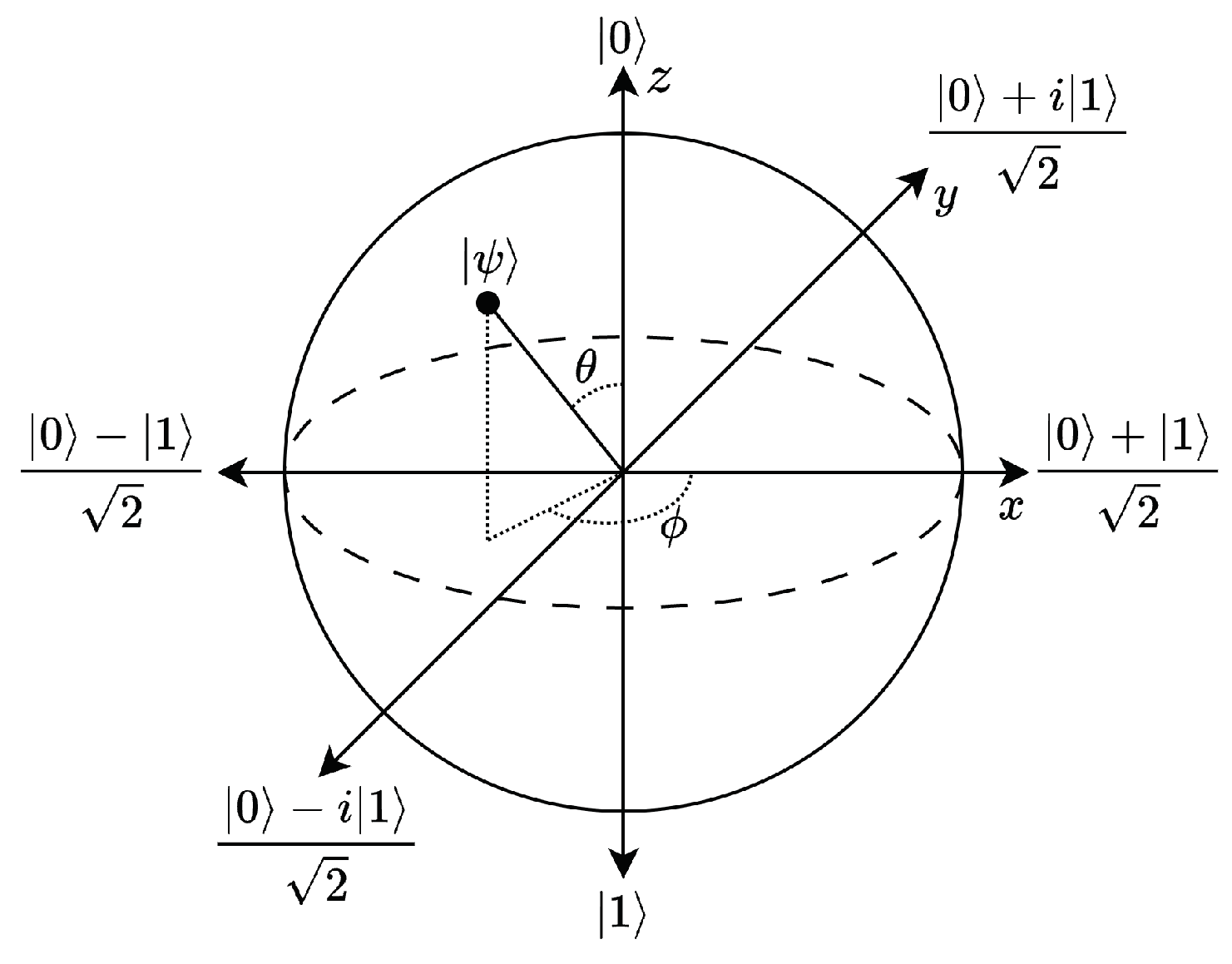
elements, called a statevector, see (1). The state of a qubit is represented as a point on the surface of the Bloch sphere [10], as shown in Figure 1. To preserve the normalization property of a statevector, a qubit’s state can only be expressed as a point on the sphere’s surface [11].

ψ = c_{0} | 0 〉 + c_{1} | 1 〉 = [\begin{matrix} c_{0} \\ c_{1} \end{matrix}], where c_{0}^{2} + c_{1}^{2} = 1

(1)

For n qubits, the statevector

ψ

has

N = 2^{n}

elements . As shown in (2), each element

c_{j} \in C

ψ

represents the amplitude/coefficient of the

j^{t h}

entry in

ψ

, or the basis state j [11].

ψ = \sum_{j = 0}^{N - 1} c_{j} \cdot j = [\begin{matrix} c_{0} \\ c_{1} \\ ⋮ \\ c_{j} \\ ⋮ \\ c_{N - 2} \\ c_{N - 1} \end{matrix}], where \sum_{j = 0}^{N - 1} | c_{j} |^{2} = 1, and 0 \leq j < (N = 2^{n})

(2)

2.2. Quantum Gates

Quantum gates are reversible operations on qubits and can be mathematically represented by unitary matrices [11]. Serial operations of quantum gates can be represented using matrix multiplication, while parallel operations can be represented using the tensor product [11]. In this section, we briefly discuss single- and multi-qubit quantum gates relevant to the proposed mqcc.

2.2.1. Rotation Gates

The rotation gates,

R_{x} (θ)

R_{y} (θ)

, and

R_{z} (ϕ)

, are parameterized versions of the Pauli single-qubit gates, shown in (3), (4), and (5), respectively [12]. In qml, rotation gate parameters are trained to produce better models [5,7].

R_{x} (θ) = [\begin{matrix} cos (\frac{θ}{2}) & - i sin (\frac{θ}{2}) \\ - i sin (\frac{θ}{2}) & cos (\frac{θ}{2}) \end{matrix}]

(3)

R_{y} (θ) = [\begin{matrix} cos (\frac{θ}{2}) & - sin (\frac{θ}{2}) \\ sin (\frac{θ}{2}) & cos (\frac{θ}{2}) \end{matrix}]

(4)

R_{z} (ϕ) = [\begin{matrix} e^{- \frac{i ϕ}{2}} & 0 \\ 0 & e^{\frac{i ϕ}{2}} \end{matrix}]

(5)

2.2.2. Hadamard Gate

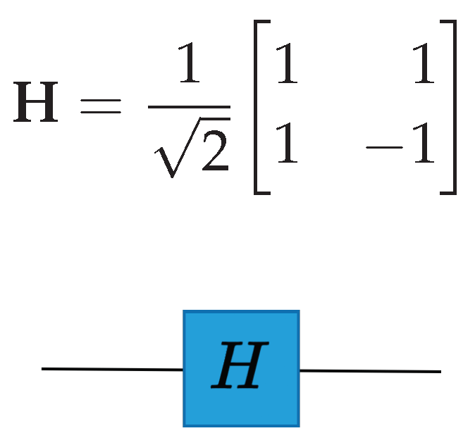
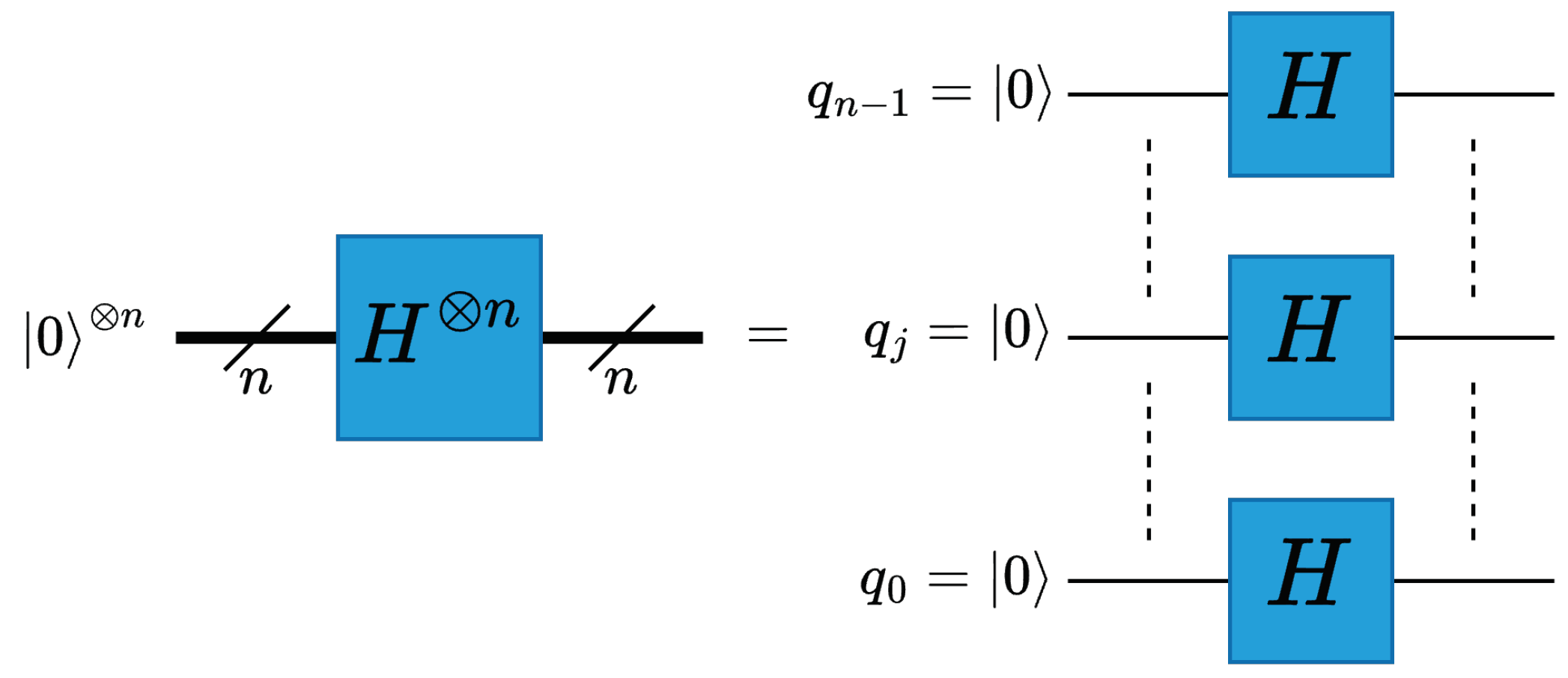
The Hadamard gate is a fundamental quantum gate that puts the qubit into a superposition of two basis states, the 0 and 1 states, see (6) and Figure 2 [11]. Similarly, by applying Hadamard gates on n qubits independently, an n-qubit superposition can be created that comprises of

2^{n}

basis states, as shown in (7) and Figure 3.

H = \frac{1}{\sqrt{2}} \begin{matrix} [r] 1 & 1 \\ 1 & - 1 \end{matrix}

(6)

H^{\otimes n} \cdot 0^{\otimes n} = \frac{1}{\sqrt{2^{n}}} \sum_{j = 0}^{2^{n} - 1} j

(7)

2.2.3. cnot Gate

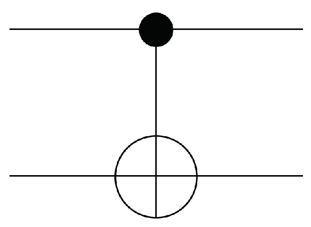
cnot gates can form a fundamental set of basis gates in conjunction with single-qubit rotation gates [12], see (8) and Figure 4. cnot gates can be used to entangle two qubits, where a measurement of one qubit can provide information about the second qubit [12].

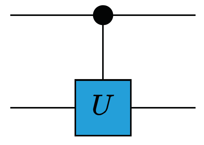
CNOT = cX = (| 0 〉 〈 0 | \otimes I) + (| 1 〉 〈 1 | \otimes X) = [\begin{matrix} 1 & 0 & 0 & 0 \\ 0 & 1 & 0 & 0 \\ 0 & 0 & 0 & 1 \\ 0 & 0 & 1 & 0 \end{matrix}]

(8)

All gates, single- or multi-qubit, can be extended to have control qubit(s), shown for a general U in (9) and Figure 5 [12].

cU = (| 0 〉 〈 0 | \otimes I) + (| 1 〉 〈 1 | \otimes U) = [\begin{matrix} I & 0 \\ 0 & U \end{matrix}]

(9)

When a general multi-qubit gate is extended to have more control qubits, it becomes an n-qubit mcu gate. In the context of cnot gates, the operation becomes a mcx gate [13]. For an n-qubit mcx gate with

n - 1

control qubits and 1 target qubit, see (10), the depth of an mcx gate with the addition of a single extra qubit can be found in (11) [13].

MCX (n) = \sum_{i = 0}^{2^{n - 1} - 2} (i i \otimes I) + (| 2^{n - 1} - 1 〉 〈 2^{n - 1} - 1 | \otimes X)

(10)

Δ_{MCX} (n) \leq 48 n - 196 = O (n) for large n

(11)

The most general controlled gate is the multiplexer, see (12), which defines a quantum operation to be applied on

n_{t a r g e t}

qubits for each state permutation of some control qubit(s),

n_{c o n t r o l}

[12]. In quantum circuits, the square box notation is used to denote a multiplexer operation, as shown in Figure 6 [12].

U_{m u x} = \sum_{i = 0}^{2^{n_{c}} - 1} | i 〉 〈 i | \otimes U_{i} = [\begin{matrix} U_{0} \\ ⋱ \\ U_{2^{n_{c o n t r o l} - 1}} \end{matrix}] \begin{matrix} ↕ 2^{n_{t a r g e t}} \\ ⋮ \\ ↕ 2^{n_{t a r g e t}} \end{matrix} ↕ 2^{n_{t a r g e t} + n_{c o n t r o l}}

(12)

Here,

U_{i}

is a matrix of size

2^{n_{t a r g e t}} \times 2^{n_{t a r g e t}}

defining the unitary operations/gates applied on each data qubit for the corresponding values i, where,

0 < i < 2^{n_{c o n t r o l} - 1}

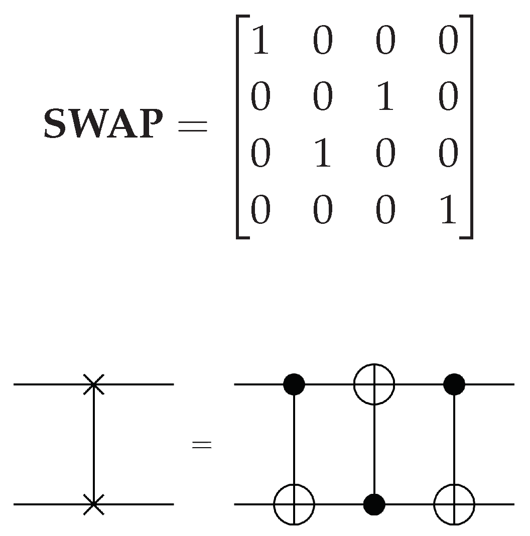
2.2.4. SWAP Gate

In a quantum circuit, SWAP gates are applied to interchange the position of two qubits, as shown in (13) and Figure 7. The SWAP gate can be decomposed into three cnot gates [11], see Figure 7.

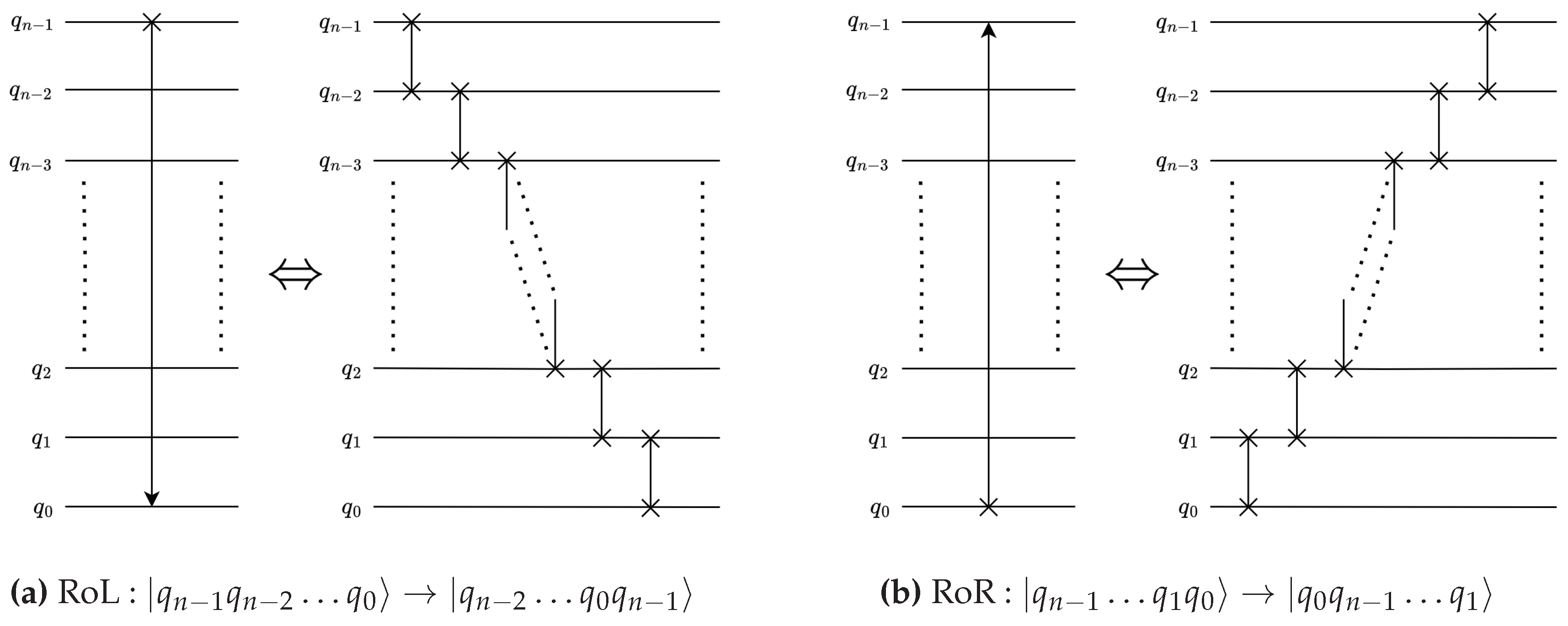
SWAP = [\begin{matrix} 1 & 0 & 0 & 0 \\ 0 & 0 & 1 & 0 \\ 0 & 1 & 0 & 0 \\ 0 & 0 & 0 & 1 \end{matrix}]

(13)

2.2.5. Quantum Perfect-Shuffle Permutation (PSP)

The quantum psp are operations that perform a cyclical rotation of given input qubits and can be implemented using SWAP gates. Figure 8 shows the rol and ror psp operations [14] with

(n - 1)

SWAP operations, or

3 (n - 1)

equivalent cnot operations.

2.2.6. Quantum Shift Operation

The quantum shift operation also performs a cyclic rotation of the basis states [15] similar to the quantum perfect-shuffle operations. Here, the basis states of the n-qubit state

ψ

are shifted by

+ k

- k

positions by applying a shift operation

U_{shift}^{\pm k}

, see (14). Here the value of k determines the type of operation such that when

k > 0

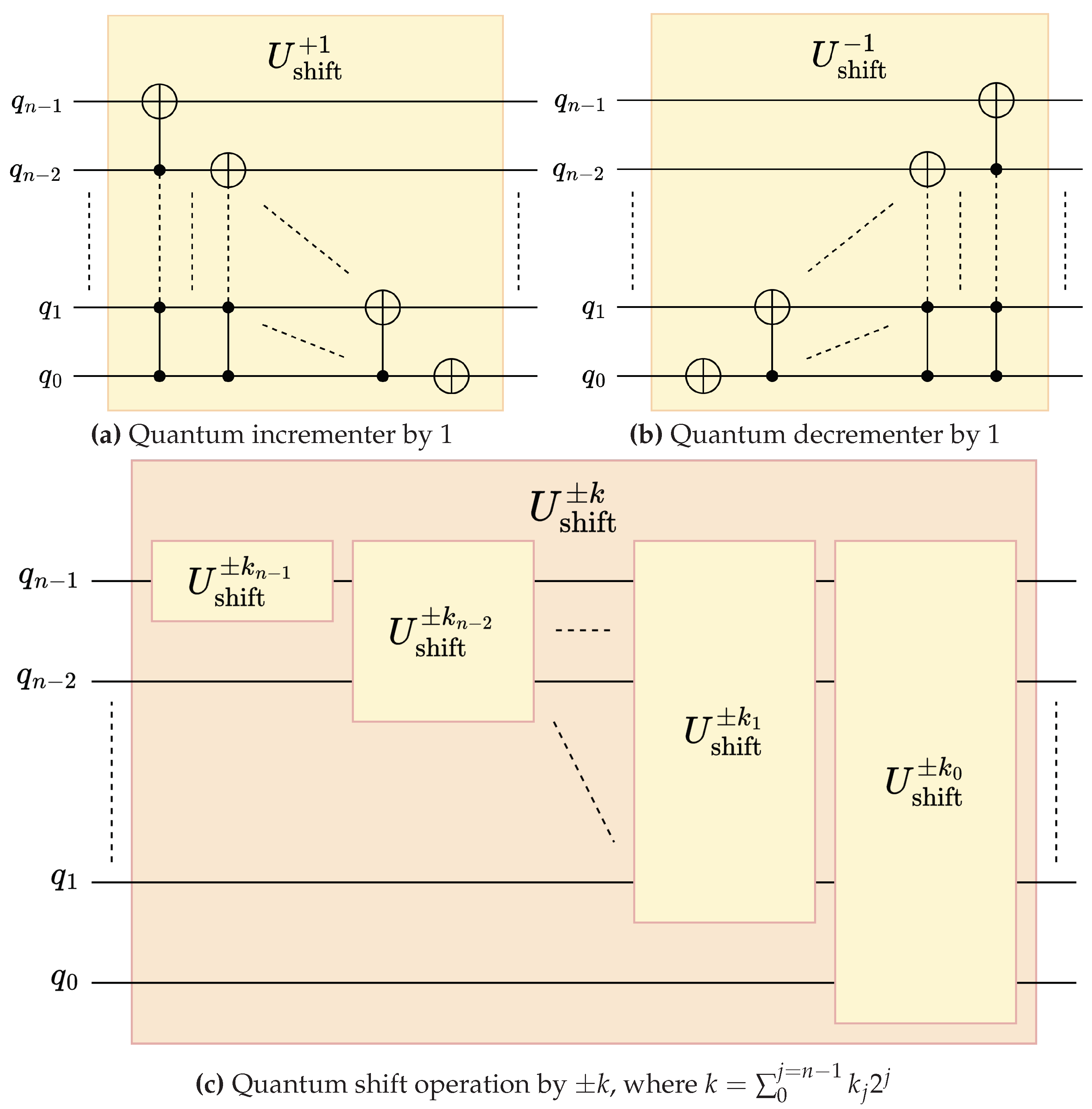
, the corresponding shift operation is denoted as a quantum incrementer, shown in Figure 9[16,17] and when

k < 0

, the corresponding shift operation is denoted as a quantum decrementer [16,17], shown in Figure 9. The quantum shift operation plays a vital role in convolution operation by striding the filter operation over data windows [18].

\begin{matrix} U_{shift}^{\pm k} ψ & = \sum_{i = 0}^{2^{n} - 1} c_{i} j, where j = (i \pm k) mod 2^{n} \\ = (\prod_{i = 0}^{k - 1} U_{shift}^{\pm 1}) ψ = {(U_{shift}^{\pm 1})}^{k} ψ \end{matrix}

(14)

Each quantum shift operation

U_{shift}^{\pm 1}

acting on an n-qubit state can be decomposed into a pyramidal structure of n×mcx gates in a series pattern [15], as shown in Figure 9 and Figure 9. In terms of fundamental single-qubit and cnot gates, the depth of a quantum shift operation with

\pm 1

can be demonstrated as quadratic [13], see (15). Generalized quantum shift operations

U_{shift}^{\pm k}

can be derived using

k \times U_{shift}^{\pm 1}

operations, from the expression in (14) and the corresponding circuit depth can be derived as shown in ().

\begin{matrix} \begin{matrix} Δ_{U_{shift}^{- 1}} (n) & = \sum_{i = 0}^{n - 1} Δ_{MCX} (i) \\ = \sum_{i = 0}^{n - 1} 48 i - 196 \\ \leq 24 n^{2} - 220 n = O (n^{2}) for large n \end{matrix} \end{matrix}

(15)

\begin{matrix} \begin{matrix} Δ_{U_{shift}^{\pm k}} (n, k) & = k \cdot Δ_{U_{shift}^{\pm 1}} (n) = O (k n^{2}) \end{matrix} \end{matrix}

(16)

Now,

U_{shift}^{\pm k}

can be expressed as a sequence of controlled shift operations, as shown in (17a). Such operations can be denoted as

U_{shift}^{\pm k_{j} 2^{j}} (n)

, where

0 \leq j < n

and

(n)

indicates that the shift operation is applied to an n-qubit state, as shown in (). Instead of applying sequential

U_{shift}^{\pm 1} (n)

operations, each

U_{shift}^{\pm 2^{j}} (n)

operation can be performed using a single

U_{shift}^{\pm 1} (n - j)

operation, see (). Therefore, a more depth-efficient decomposition is shown in Figure 9 and the corresponding depth is provided in ().

\begin{matrix} \begin{matrix} k & = {(k_{n - 1} k_{n - 2} \dots k_{j} \dots k_{1} k_{0})}_{2} = \sum_{j = 0}^{n - 1} k_{j} 2^{j} : k_{j} \in {0, 1} \end{matrix} \end{matrix}

(17a)

\begin{matrix} \begin{matrix} U_{shift}^{\pm k} (n) & = U_{shift}^{\pm \sum_{j = n - 1}^{0} k_{j} 2^{j}} (n) = \prod_{j = n - 1}^{0} U_{shift}^{\pm k_{j} 2^{j}} (n) \\ = \prod_{j = n - 1}^{0} (U_{shift}^{\pm k_{j}} (n - j) \otimes I^{\otimes j}) \end{matrix} \end{matrix}

(17b)

\begin{matrix} \begin{matrix} Δ_{U_{shift}^{\pm k}}^{opt} (n) & \leq \sum_{j = 0}^{n - 1} Δ_{U_{shift}^{- 1}} (n - j) = 24 \sum_{j = 0}^{n - 1} j^{2} - 220 \sum_{j = 0}^{n - 1} j \\ \leq 8 n^{3} - 122 n^{2} + 114 n = O (n^{3}) for large n \end{matrix} \end{matrix}

(17c)

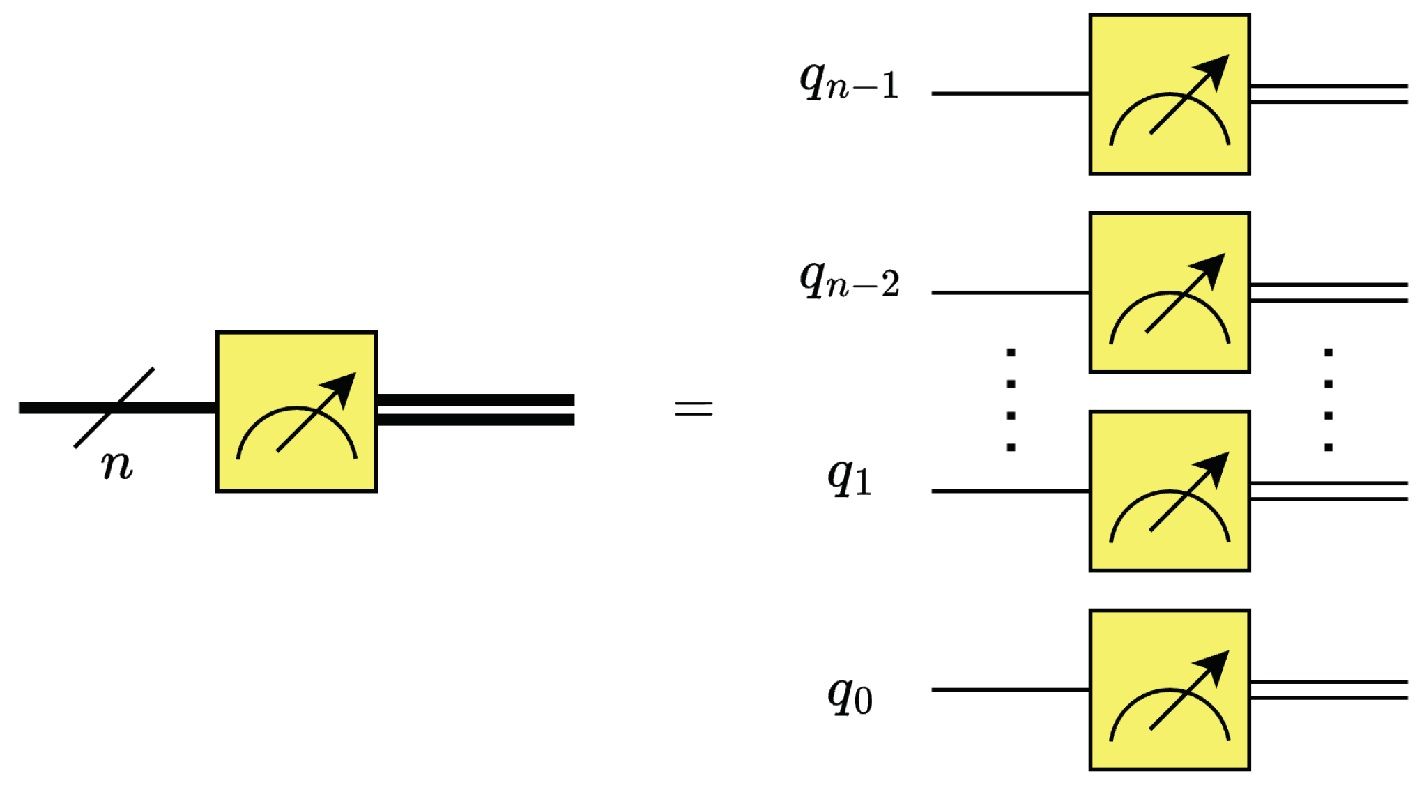
2.3. Quantum Measurement and Reset

The quantum measurement operation of a qubit, is usually and informally referred to as a measurement “gate“. The measurement gate is a non-unitary operation that can project the quantum state of a qubit

ψ

to the 0 or 1 basis states [11]. The likelihood of measuring any basis state can be obtained by taking the squared magnitude of their corresponding basis state coefficient. For a n-qubit register

ψ

with

2^{n}

possible basis states, the probability of measuring each qubit in any particular basis state j, where

0 \leq j < 2^{n}

, is given by

| c_{j} |^{2}

[14]. The classical output of an n-qubit amplitude-encoded [19] data can be decoded as

ψ_{decoded - data}^{classical}

. This classical output vector can be reconstructed by the square root of the probability distribution

\sqrt{P (ψ)}

, as shown in (18), (19) and Figure 10. When amplitude-encoding [19] is used for encoding positive real classical data, the coefficients of the corresponding quantum pure state [11]

ψ

are also positive real, i.e.,

c_{j} \in R^{+}

, where

0 \leq j < 2^{n}

. Thus, the amplitudes of

ψ

are numerically equal in values to the coefficients of

ψ_{decoded - data}^{classical}

, i.e.,

ψ = ψ_{decoded - data}^{classical}

. Therefore, the quantum state

ψ

can be completely determined from the measurement probability distribution such that

ψ = \sqrt{P (ψ)}

only when the amplitudes of the quantum state are all of positive real values. Moreover, the probability distribution

P (ψ)

can be reconstructed by repeatedly measuring (sampling) the quantum state

ψ

. In general, an order of

2^{n}

measurements is required to accurately reconstruct the probability distribution. In order to reduce the effects of quantum statistical noise, it is recommended to gather as many circuit samples (shots) [20] as possible.

P (ψ) = \begin{matrix} p_{0} \\ p_{1} \\ ⋮ \\ p_{j} \\ ⋮ \\ p_{N - 2} \\ p_{N - 1} \end{matrix} = \begin{matrix} | c_{0} |^{2} \\ | c_{1} |^{2} \\ ⋮ \\ | c_{j} |^{2} \\ ⋮ \\ | c_{N - 2} |^{2} \\ | c_{N - 1} |^{2} \end{matrix}, where p_{j} = {| c_{j} |}^{2}, and 0 \leq j < N

(18)

ψ_{decoded - data}^{classical} = \sqrt{P (ψ)} = \begin{matrix} | c_{0} | \\ | c_{1} | \\ ⋮ \\ | c_{j} | \\ ⋮ \\ | c_{N - 2} | \\ | c_{N - 1} | \end{matrix}

(19)

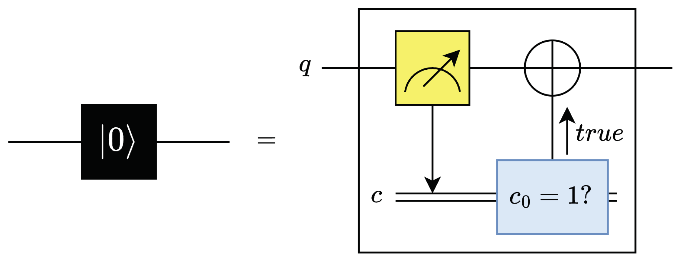
The reset operation sets the state of qubits to 0. This operation consists of a mid-circuit measurement gate followed by a conditional X gate [21,22] such that the bit-flip operation is applied when the measured qubit is in state 1. The reset gate and its equivalent circuit are both shown in Figure 11 [22].

2.4. Classical-to-Quantum (C2Q)

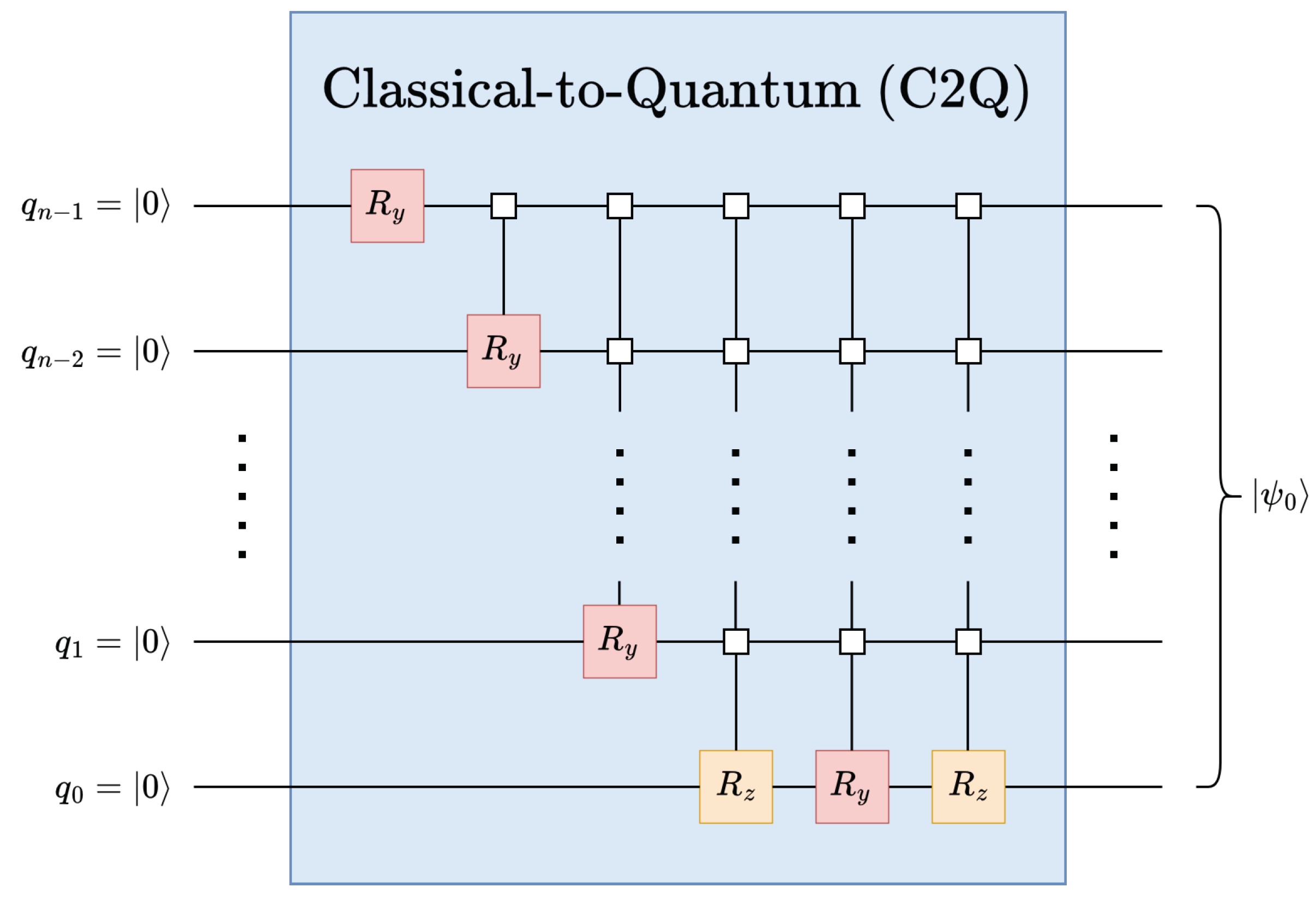
There are a number of quantum data encoding techniques [19,23], each of which uses different methods to initialize quantum circuits from the ground state. Among the many methods, this work leverages the classical-to-quantum (C2Q) arbitrary state synthesis [19,23] operation to perform amplitude encoding and initialize an n-qubit state

ψ_{0}

, see Figure 12. The c2q operation employs a pyramidal structure of multiplexed

R_{y}

and

R_{z}

gates. It should be noted that the

R_{z}

gates are only required for positive real data. Thus, for positive real data, the circuit depth is

2 \cdot 2^{n} - n - 2

, while for complex data, the circuit depth is

3 \cdot 2^{n} - n - 4

[19].

2.5. Quantum Machine Learning with Variational Algorithms

Variational quantum algorithms are a type of quantum-classical techniques that facilitate implementations of machine learning on noisy-intermediate-scale-quantum (nisq) machines [5,7]. Current quantum devices are not able to maintain coherent states for sufficient periods, preventing current algorithms from performing meaningful optimization on the machine learning model. Thus, vqa combine classical optimization algorithms with parameterized quantum circuits, or ansatz. Here, the ansatz takes on the role of the model [5]. One specific type of vqa is the vqc, which is used for classification problems. Existing vqc [6,8,9] have been shown to be effective for classifying datasets with high accuracy and few training parameters in both simulation and current quantum processors.

3. Related Work

In this section, we discuss the existing related works with an emphasis on quantum machine learning. Our discussion focuses on commonly used Data Encoding techniques, existing implementations of the Convolution and Quantum Convolution algorithms, and related Quantum Machine Learning algorithms. Moreover, we also discuss existing quantum convolutional classification algorithms that leverage data locality.

3.1. Data Encoding

For encoding classical image data into the quantum domain, the commonly used methods are frqi [24] and the neqr [25]. In frqi, positional and color information are encoded as amplitude encoding and angle encoding respectively. In neqr, positions of the pixels are encoded using amplitude encoding but color information is encoded using basis encoding, where q represents the number of bits/qubits allocated for color data. For

N = 2^{n}

data points, in terms of circuit width and depth, frqi incurs

n + 1

and

O (4^{n})

, respectively, while neqr incurs

n + q

and

O (q n 2^{n})

, respectively [15]. Although these techniques are employed in the existing quantum convolution techniques, their disadvantages are discussed below.

3.2. Convolution

We now discuss existing implementations of convolution and discuss their associated time complexity. These implementations consist of various classical and quantum techniques. In addition, we consider the shortcomings of existing quantum convolution methods.

3.2.0.1. Classical Convolution

Classical implementations of convolution are usually implemented directly, through gemm, or through the fft. For a data size N, running the direct implementation on CPUs has complexity

O (N^{2})

[26], while the complexity of an fft-based implementation is

O (N log N)

[26]. On GPUs, fft-based convolution incurs a similar

O (N log N)

complexity [27], while the direct approach requires

O (N_{F} N)

FLOPS [28,29], where

N_{F}

is the filter size.

3.2.0.2. Quantum Convolution

The existing quantum convolution techniques [18,30,31,32,33] rely on fixed filter sizes and support only specific filters at a time, e.g., edge-detection. They do not contain methods for implementing a general filter. Additionally, these techniques have a quadratic circuit depth, i.e.,

O (n^{2})

, where

n = ⌈ {log}_{2} N ⌉

is the number of qubits and N is the size of the input data. While these methods appear to show quantum advantage, these results do not include overhead incurred from data encoding. The related methods employ the FRQI and NEQR data encoding methods, leading to inferior performance compared to classical methods once the additional overhead is factored in. The authors in [16] propose an edge-detection technique based on quantum wavelet transform QWT and amplitude encoding, named quantum Hadamard edge detection (QHED) which is not generalizable for multiple convolution kernels or multidimensional data. Thus, their algorithm loses parallelism, increases circuit depth, and is difficult to generalize beyond capturing 1D features. In [15], the authors have developed a quantum convolution algorithm that supports single feature/kernel and multidimensional data. In this work, we leverage the convolution method from [15] and generalize it to support multiple features/kernels in our proposed MQCC framework.

3.3. Quantum Machine Learning

There exist two primary techniques for quantum convolutional classification that may leverage data locality through convolution: qcnn [34] and quanvolutional neural networks [35]. QCNN is inspired by classical convolutional neural networks, employs quantum circuits to perform convolutions, while quanvolutional neural networks replace classical convolutional layers with quantum convolutional (or quanvolutional) layers.

3.3.1. Quantum Convolutional Neural Networks

The qcnn [34] and our proposed mqcc are both vqa with structures inspired by cnns. However, qcnn borrows the superficial structure of cnns without considering the underlying purpose. Specifically, the qcnn quantum ansatz is designed so that its "convolution" and "pooling" operations exploit the locality of qubits in the circuit (rather than the locality of data). However, unlike data locality, qubit locality does not have a practical purpose for machine learning in terms of isolating relevant input features. Moreover, by considering input data as 1D, qcnn do not leverage the dimensionality of datasets, which constitute a primary advantage of cnn. mqcc, on the other hand, faithfully implements cnn operations in quantum circuits, offering performance improvements in computational speed and classification accuracy even over contemporary implementations on classical computers.

3.3.2. Quanvolutional Neural Networks

Quanvolutional neural networks [35] are a hybrid quantum-classical algorithm named eponymously after the quanvolutional layer added to a conventional cnn. These quanvolutional layers serve to decimate a 2-D image, which is then sequentially fed into a quantum device. In this manner, the quanvolutional layer effectively exploits data locality. Yet, the model’s dependency on classical operations, specifically the decimation of input data and the repeated serial data I/O transfer, vastly increases compute time. In contrast, the required convolution operation is incorporated into our proposed mqcc, reducing classical-quantum data transfer. Moreover, mqcc takes advantage of parallelism inherent to quantum computers, while quanvolutional neural networks do not. Together, this allows the mqcc to apply convolutional filters to window data in parallel.

4. Materials and Methods

In this section, we describe the materials and methods associated with the proposed mqcc. The proposed method mainly uses generalized quantum convolution, quantum pooling based on the qht and partial measurement [14], and a quantum fully-connected layer that will be illustrated in this section. To the best of our knowledge, this work is the first to:

Develop a generalizable quantum convolution algorithm for a quantum convolution-based classifier that supports multiple features/kernels.
Design a scalable mqcc that uses multidimensional quantum convolution and pooling based on the qht. This technique reduces training parameters and time complexity compared to other classical and quantum implementations.
Evaluate the mqcc model in a state-of-the-art QML simulator from Xanadu using a variety of datasets.

4.1. Quantum Fully-Connected Layer

A fully-connected neural network constitutes a collection of layers that each perform a linear transformation on

N_{in}

input features

x \in R^{N_{in}}

to generate

N_{out}

-feature output

y \in R^{N_{out}}

[2,3]. Each layer can be represented in terms of a multiply-and-accumulate (MAC) operation and an addition operation as shown in (20), where

W \in R^{N_{out} \times N_{in}}

and

b \in R^{N_{out}}

represent the trainable weight and bias parameters, respectively.

y = W^{T} x + b

(20)

The particular weights and biases that generate the

j^{th}

feature of the output,

y_{j}

, can be isolated by taking the

j^{th}

column of

W

w_{j}

, and the

j^{th}

term of

b

b_{j}

, as shown in (21), which can be directly implemented using quantum circuits. Section 4.1.1 discusses the quantum circuits for a single-feature output, and Section 4.1.2 generalizes the proposed technique for an arbitrary amount of features in the output.

\begin{matrix} y_{j} = (w_{j} \cdot x) + b_{j}, where 0 \leq j < N_{out} \end{matrix}

(21)

4.1.1. Single-Feature Output

For a single-feature output neural network, the weight parameters can be represented as a vector

w \in R^{N_{in}}

. Here

w

can be expressed as a quantum state w as shown in (22) similar to the process of C2Q data encoding, see Section 2.4.

\begin{matrix} w & = \frac{1}{w} [\begin{matrix} w \\ 0 \\ ⋮ \\ 0 \end{matrix}] \begin{matrix} [l] ↕ N_{in} \end{matrix}↕ 2^{n_{in}}, where n_{in} = ⌈ {log}_{2} N_{in} ⌉ \end{matrix}

(22)

Similarly, for a single-feature output, Dirac notation of the MAC operation follows from (21) as shown in (23), where

ψ

corresponds to the input data.

y - b = w ψ

(23)

However, it is necessary to obtain a quantum operator to perform a parameterized unitary linear transformation from the weights vector w on the input data

ψ

using an inverse C2Q operation, as shown in (24).

\begin{matrix} U_{MAC} (w) & = [\begin{matrix} w \\ \times \\ ⋮ \\ \times \end{matrix}]↕ 2^{n_{in}} \\ = U_{C 2 Q}^{†} (w) \end{matrix}

(24)

4.1.2. Multi-Feature Output

A Multi-Feature Output can be implemented in a naive approach using Single-Feature Output (24) for an

N_{out}

-feature output, where

N_{out} \leq N_{in}

, which can be obtained by encoding each weight vector

w_{j} : 0 \leq j < N_{out}

as a normalized row in

U_{MAC}

. However, the result might yield a non-unitary operator as the weight vectors can be arbitrary.

U_{MAC}

is unitary when each row is orthogonal to all other rows in the matrix, mathematically,

W_{i} W_{j} = δ_{i j} : \forall i, j \in [0, N_{out})

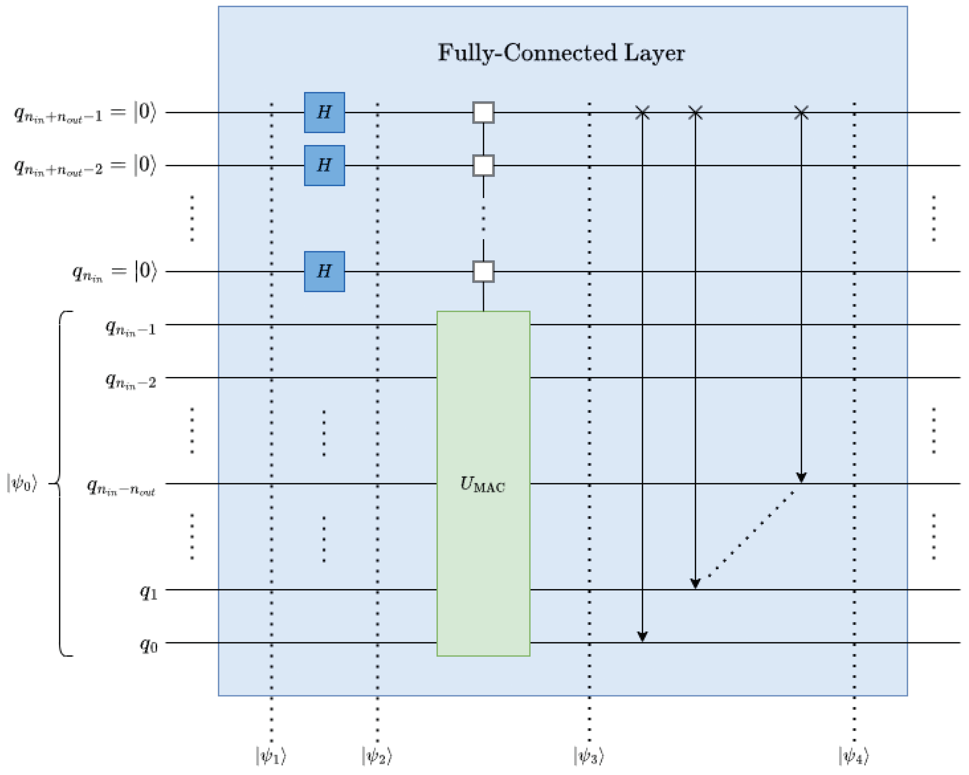
. As described in Section 2.2.3, independently-defined weights can be supported for each feature of the output by multiplexing

U_{MAC}

. Now, the generic fully-connected operation,

U_{FC}

, can be generated as shown in (25), where

n_{out} = ⌈ {log}_{2} N_{out} ⌉

U_{FC} = [\begin{matrix} U_{MAC} (w_{0}) \\ ⋱ \\ U_{MAC} (w_{2^{n_{out}} - 1}) \end{matrix}]

(25)

By generating

N_{out}

replicas of the initial state,

ψ_{0}

, the operation can be parallelized, i.e.,

U_{MAC} (w_{0}) \dots U_{MAC} (w_{2^{n_{out}} - 1})

transformations from (25).

4.1.2.1. Replication:

To replicate the initial state,

ψ_{0}

n_{out}

qubits, which extend the statevector to a total size of

2^{n_{in} + n_{out}}

, see (26) and Figure 14.

ψ_{1} = 0^{\otimes n_{out}} \otimes ψ_{0} = [\begin{matrix} ψ_{0} \\ 0 \\ ⋮ \\ 0 \end{matrix}] \begin{matrix} [l] ↕ 2^{n_{in}} \end{matrix}↕ 2^{n_{in} + n_{out}}

(26)

By applying an

n_{out}

-qubit Hadamard operation to the relevant qubits the replicas can be obtained through superposition, see (27) and Figure 14, which generates the desired replicas scaled by a factor of

\frac{1}{\sqrt{2^{n_{out}}}}

to maintain normalization

ψ_{2} = 1

\begin{matrix} ψ_{2} = (H^{\otimes n_{out}} \otimes I^{\otimes n_{in}}) ψ_{1} = \frac{1}{\sqrt{2^{n_{out}}}} [\begin{matrix} ψ_{0} \\ ⋮ \\ ψ_{0} \end{matrix}] \begin{matrix} [l] ↕ 2^{n_{in}} \\ ⋮ \\ ↕ 2^{n_{in}} \end{matrix}↕ 2^{n_{in} + n_{out}} \end{matrix}

(27)

4.1.2.2. Applying the $U_{FC}$ Filter:

U_{FC}

can perform the MAC operation for the entire

N_{out}

-feature output in parallel with the set of replicas of

ψ_{0}

, see, (28) and Figure 14.

\begin{matrix} ψ_{3} = U_{FC} ψ_{2} & = [\begin{matrix} U_{MAC} (w_{0}) ψ_{0} \\ ⋮ \\ U_{MAC} (w_{j}) ψ_{0} \\ ⋮ \\ U_{MAC} (w_{2^{n_{out}} - 1}) ψ_{0} \end{matrix}] \begin{matrix} [l] ↕ 2^{n_{in}} \\ ⋮ \\ ↕ 2^{n_{in}} \\ ⋮ \\ ↕ 2^{n_{in}} \end{matrix}↕ 2^{n_{in} + n_{out}} \\ = [\begin{matrix} w_{0} ψ_{0} \\ \times \\ ⋮ \\ \times \\ ⋮ \\ w_{j} ψ_{0} \\ \times \\ ⋮ \\ \times \\ ⋮ \\ w_{2^{n_{out}} - 1} ψ_{0} \\ \times \\ ⋮ \\ \times \end{matrix}] \begin{matrix} [l] ↕ 2^{n_{in}} \\ ⋮ \\ ↕ 2^{n_{in}} \\ ⋮ \\ ↕ 2^{n_{in}} \end{matrix}↕ 2^{n_{in} + n_{out}} \end{matrix}

(28)

4.1.2.3. Data Rearrangement:

The data rearrangement operation can be performed by applying perfect-shuffle gates, see Section 2.2.5. It simplifies the output-feature extraction by gathering them into

N_{out}

data points at the top of the statevector, see (29) and Figure 14.

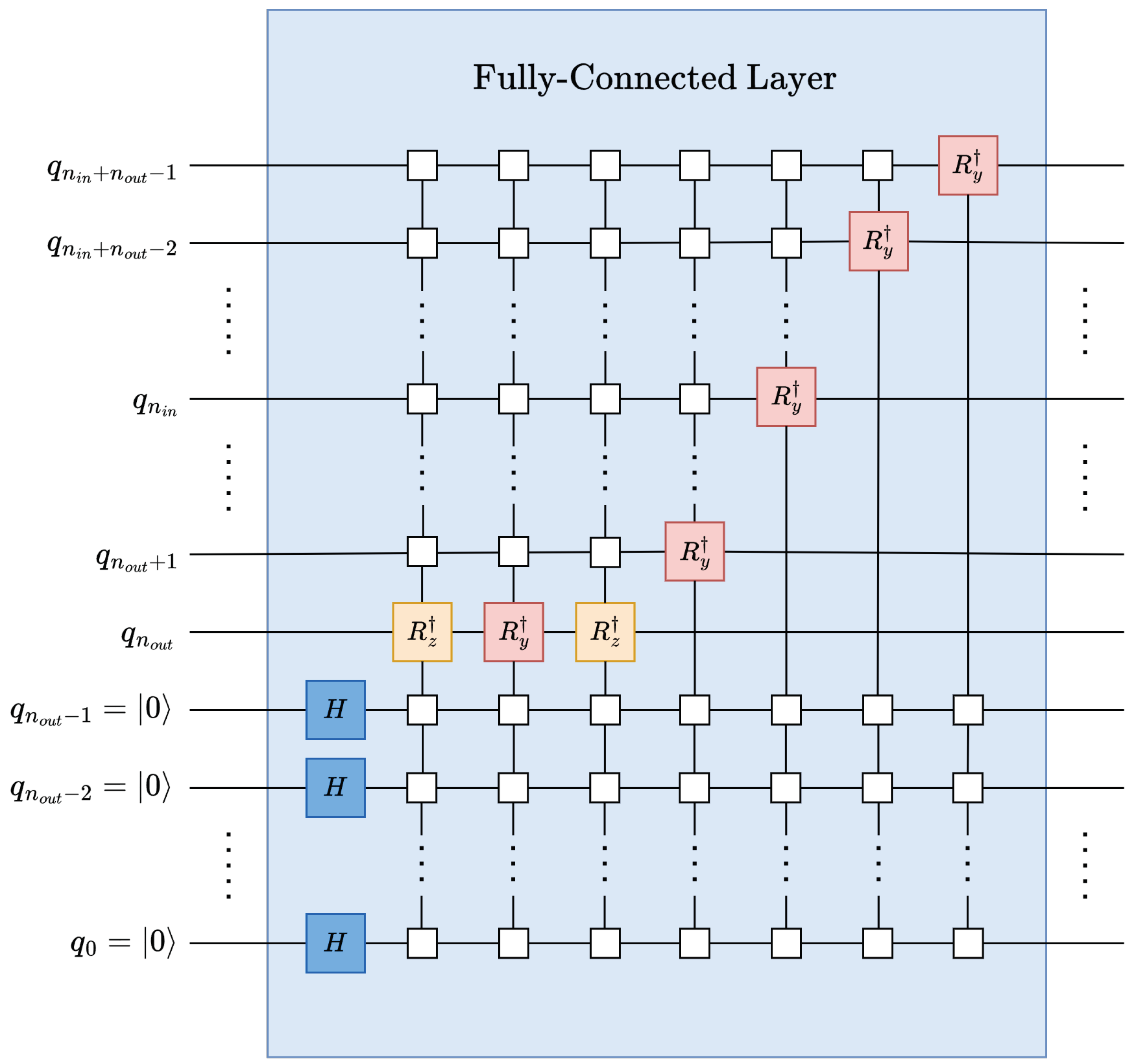
\begin{matrix} ψ_{4} = \prod_{i = 0}^{n_{out} - 1} (RoL (n_{in} + n_{out} - i) \otimes I^{\otimes i}) ψ_{3} & = [\begin{matrix} w_{0} ψ_{0} \\ ⋮ \\ w_{j} ψ_{0} \\ ⋮ \\ w_{2^{n_{out}} - 1} ψ_{0} \\ \times \\ ⋮ \\ \times \end{matrix}] \begin{matrix} [l] ↕ 2^{n_{out}} \end{matrix}↕ 2^{n_{in} + n_{out}} \end{matrix}

(29)

It is worth mentioning that instead of applying the auxiliary qubits at the most-significant position as shown in the decomposed and simplified fully-connected circuit in Figure 15, auxiliary qubits can be applied at the least-significant position to avoid perfect-shuffle permutations.

4.1.3. Circuit Depth of the Quantum Fully-Connected Layer

As discussed in Section 2.4,

U_{MAC}

operation is implemented by applying the C2Q / arbitrary state synthesis operation with a depth of

(3 \cdot 2^{n_{in}} - n_{in} - 4)

fundamental single-qubit and CNOT gates. The depth is expected to increase by a factor of

2^{n_{out}}

when multiplexing

U_{MAC}

to implement an

N_{out}

-feature output [12], see (30).

\begin{matrix} Δ_{U_{FC}} (n_{in}, n_{out}) & = 2^{n_{out}} \cdot Δ_{U_{MAC} (n_{in})} \\ = 2^{n_{out}} (3 \cdot 2^{n_{in}} - n_{in} - 4) \\ = O (2^{n_{in} + n_{out}}) \end{matrix}

(30)

4.2. Generalized Quantum Convolution

The most significant part of the mqcc framework is the generalized quantum convolution operation with support for arbitrary, parameterized filters. Compared to the classical convolution operation, the convolution operation in the quantum domain achieves exponential improvement in time complexity due to its innate parallelism. The convolution operation consists of stride, data rearrangement, and multiply-and-accumulate (MAC) operations.

4.2.0.1. Stride:

The first step of quantum convolution is generating shifted replicas of the input data. Quantum decrementers controlled by additional qubits, called "filter" qubits are used for this purpose. The

U_{shift}^{- 1}

operator as shown in Figure 9 shifts the replica by a single stride.

4.2.0.2. Multiply-and-Accumulate (MAC):

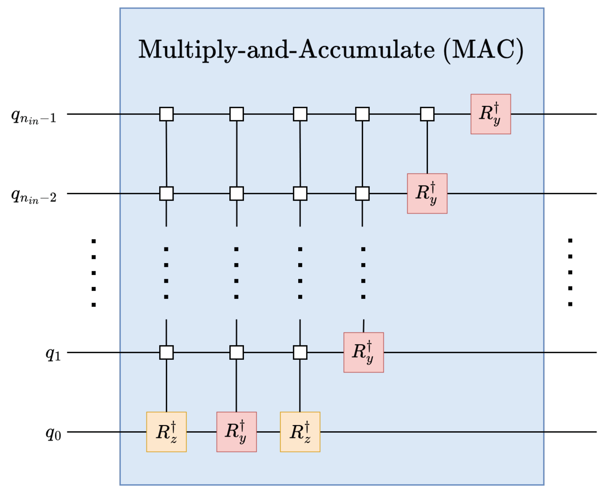
Kernels are applied to the strided replicas of the input data in parallel using the MAC operation, see Figure 13. In the MAC operations, kernels are applied to the contiguous set of data with the help of the inverse arbitrary state synthesis operation. One benefit achieved from using this MAC operation is the superposition of multiple kernels. The superposition of the kernel can be helpful for the classification of multiple features.

4.2.0.3. Data Rearrangement:

Data rearrangement is required to coalesce the output pieces of the MAC steps and create one contiguous piece of output. This step is performed using perfect shuffle permutation (PSP) operations described in Section 2.2.5.

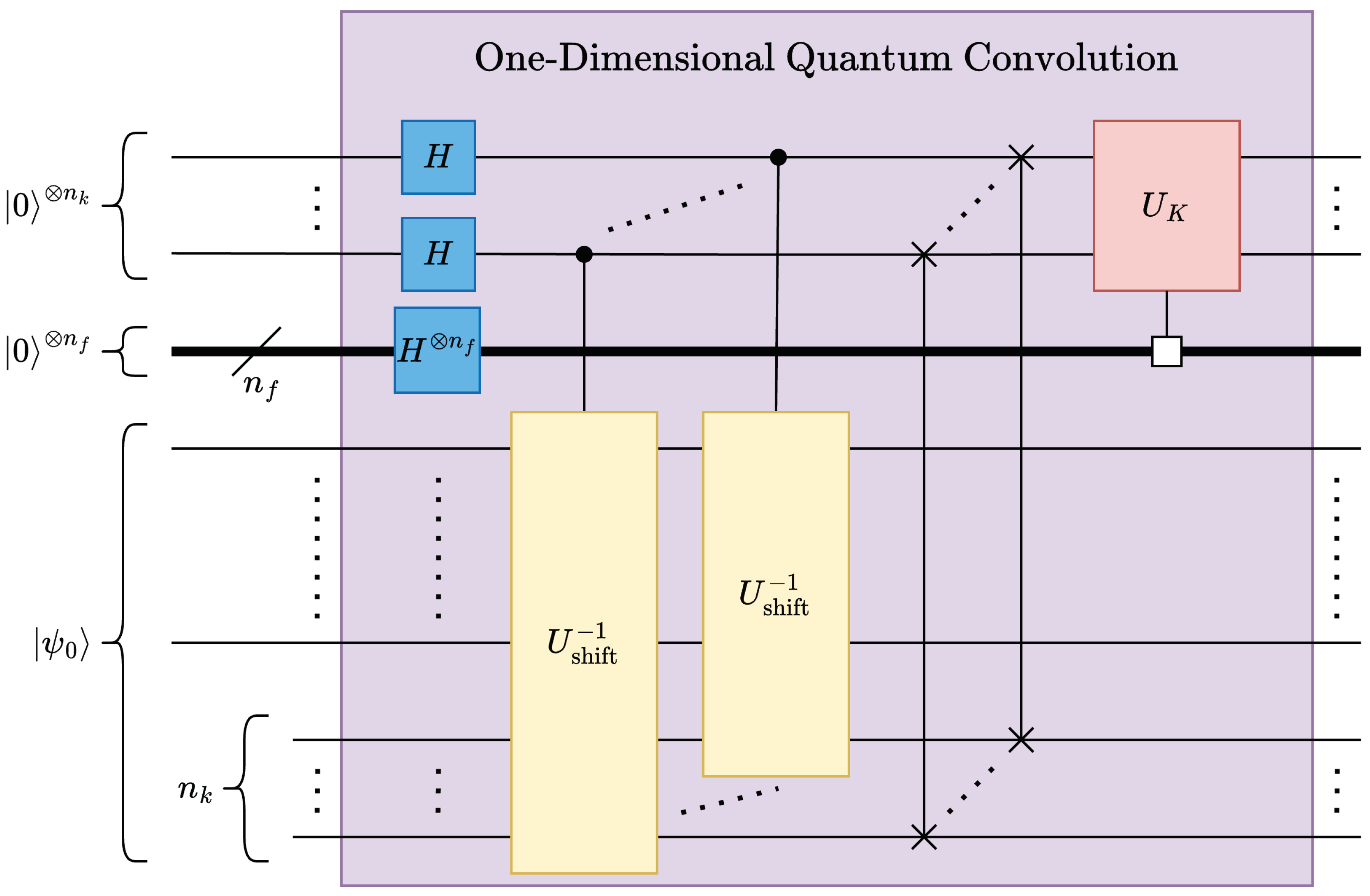
4.2.1. One-Dimensional Multi-Feature Quantum Convolution

The one-dimensional quantum convolution operation, with kernel of size

N_{K}

terms, requires generating

N_{K}

replicas of the input data in a range of possible strides between

0 \leq k < N_{K}

. Therefore, a total of

N_{K} N

terms need to be encoded into a quantum circuit including the

n_{k} = ⌈ {log}_{2} N_{K} ⌉

additional auxiliary qubits, denoted as “kernel” qubits that are allocated the most-significant qubits to maintain data contiguity.

Necessary

N_{K}

replicas of the input vector are created by using Hadamard gates, see Figure 16. Convolution kernels can be implemented using multiply-and-accumulate (MAC) operations; as such, it is possible to leverage

U_{MAC}

as defined in Section 4.1 for implementing quantum convolution kernels. Given a kernel

K \in R^{N_{K}}

, the corresponding kernel operation

U_{K}

can be constructed from the normalized kernel K as shown in (31).

U_{K} = U_{MAC} (K), where K = \hat{K} = \frac{K}{K}

(31)

When applied to the

n_{k}

lower qubits of the state vector,

U_{K}

applies the kernel

K

to all data windows in parallel. However, in CNNs, convolution layers typically must support multiple convolution kernels/ features. Fortunately, one major advantage of the proposed quantum convolution technique is that multiple features can be supported by multiplexing only the MAC operations – the stride and data rearrangement operations do not need to be multiplexed, see Figure 16. Accordingly, for

N_{F}

features,

n_{f} = ⌈ {log}_{2} N_{F} ⌉

must be added to the circuit and placed in superposition using Hadamard gates, similar to the process in (26). The depth of the proposed multi-feature 1-D quantum convolution can be obtained as (32).

\begin{matrix} Δ_{1 - D conv} (n, n_{k}) & = O (n_{k} n^{2} - n_{k}^{2} n + 2^{n_{f} + n_{k}}), where n ≫ n_{f}, n_{k} \end{matrix}

(32)

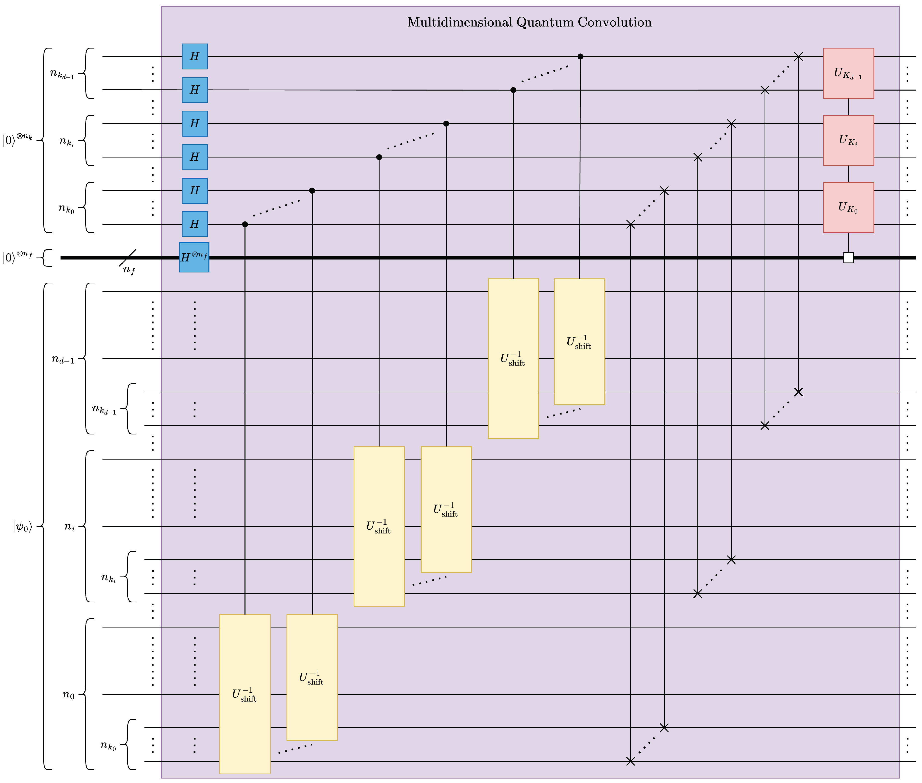
4.2.2. Multi-Dimensional Multi-Feature Quantum Convolution

Multi-dimensional quantum convolution can be implemented by stacking multiple one-dimensional quantum circuits as shown in Figure 17. A d-dimensional quantum convolution circuit can be constructed with a stacked kernel of 1-dimensional convolution circuits only when the multidimensional kernels are outer products of d instances of 1-dimensional kernels. The depth of d-D quantum convolution can be obtained as (33).

\begin{matrix} Δ_{d - D conv} (n, n_{k}) & = O (n_{k_{\max}} n_{\max}^{2} - n_{k_{\max}}^{2} n_{\max} + 2^{n_{k} + n_{f}}), where \\ n_{\max} & = {max}_{i = 0}^{d - 1} (n_{i}), n_{k_{\max}} = {max}_{i = 0}^{d - 1} (n_{k_{i}}), and n_{\max} ≫ n_{f}, n_{k_{\max}} \end{matrix}

(33)

4.3. Quantum Pooling

A critical part of cnn is the pooling operation or downsampling of the feature maps. One widely-used method is average pooling, where only the average of the adjacent pixels in the feature map is preserved, creating a smoothing effect [36].

4.3.1. Quantum Average Pooling using Quantum Haar Transform

The average pooling operation can be implemented using the qwt [14] which has the advantage of preserving data locality using wavelet transform decomposition. It is a commonly used technique for dimension reduction in image processing [14]. In this work, we utilize the simplest and first wavelet transform, quantum Haar transform (QHT) [14] to implement quantum pooling operation. This operation is executed in 2 steps: the Haar wavelet operation and data rearrangement.

4.3.1.1. Haar Wavelet Operation:

For separating the high and low-frequency components from the input data, H gates are applied in parallel. The number of H gates applied in QHT is equal to the levels of decomposition.

4.3.1.2. Data Rearrangement:

After separating the high- and low-frequency components, quantum rotate-right (RoR) operations are applied to group them accordingly.

As mentioned before, the proposed framework is highly parallelizable regardless of the dimensions of the data as the QHT operation can be applied to multiple dimensions of data in parallel.

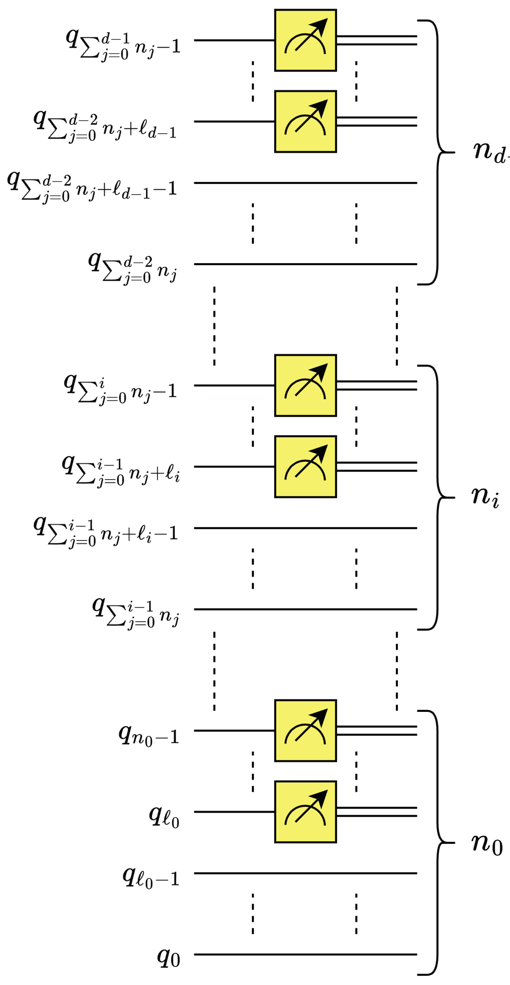
As shown in Figure 18, for a single-level of decomposition, H gates are applied on one qubit (the least significant qubit) per dimension, and for ℓ-level decomposition, shown in Figure 18, l number of H gates are applied per dimension. Each level of decomposition reduces the size of the corresponding dimension by a factor of 2.

4.3.2. Quantum Euclidean Pooling using Partial Measurement

In machine learning applications, the average and maximum (max) pooling [36] are the most commonly used pooling schemes for dimension reduction. The two schemes differ in the sharpness of data features. On one hand, max pooling yields a sharper definition of input features which makes it preferable for edge detection and certain classification applications [36]. On the other hand, average pooling offers a smoother dimension reduction that may be preferred in other workloads [36]. Thus, to accompany our implementation of quantum averaging pooling using QHT, see Section 4.3.1, it would be beneficial to have an implementation of quantum max pooling. However, such an operation would be non-unitary, creating difficulty for the implementation of quantum max pooling [37]. Therefore, instead of max pooling, we utilize an alternative pooling technique we denote as quantum Euclidean pooling.

Mathematically, average and Euclidean pooling are special cases of the p-norm [38], where for a vector of size N elements, the p-norm or

ℓ^{p}

norm of a vector

x \in C^{N}

is given by (34) for

p \in Z

[38]. The average pooling occurs for the 1-norm (

p = 1

) and Euclidean pooling occurs for the 2-norm (

p = 2

). A notable benefit of the Euclidean pooling technique is its zero-depth circuit implementation by leveraging partial measurement [37].

x_{p} = {(\sum_{i = 0}^{N} x_{i}^{p})}^{\frac{1}{p}}

(34)

This work leverages the multilevel, d-dimensional quantum Euclidean pooling circuit presented in [37], see Figure 19.

Here, for each dimension i,

ℓ_{i}

is the number of decomposition levels for dimension where

0 \leq i < d

[37].

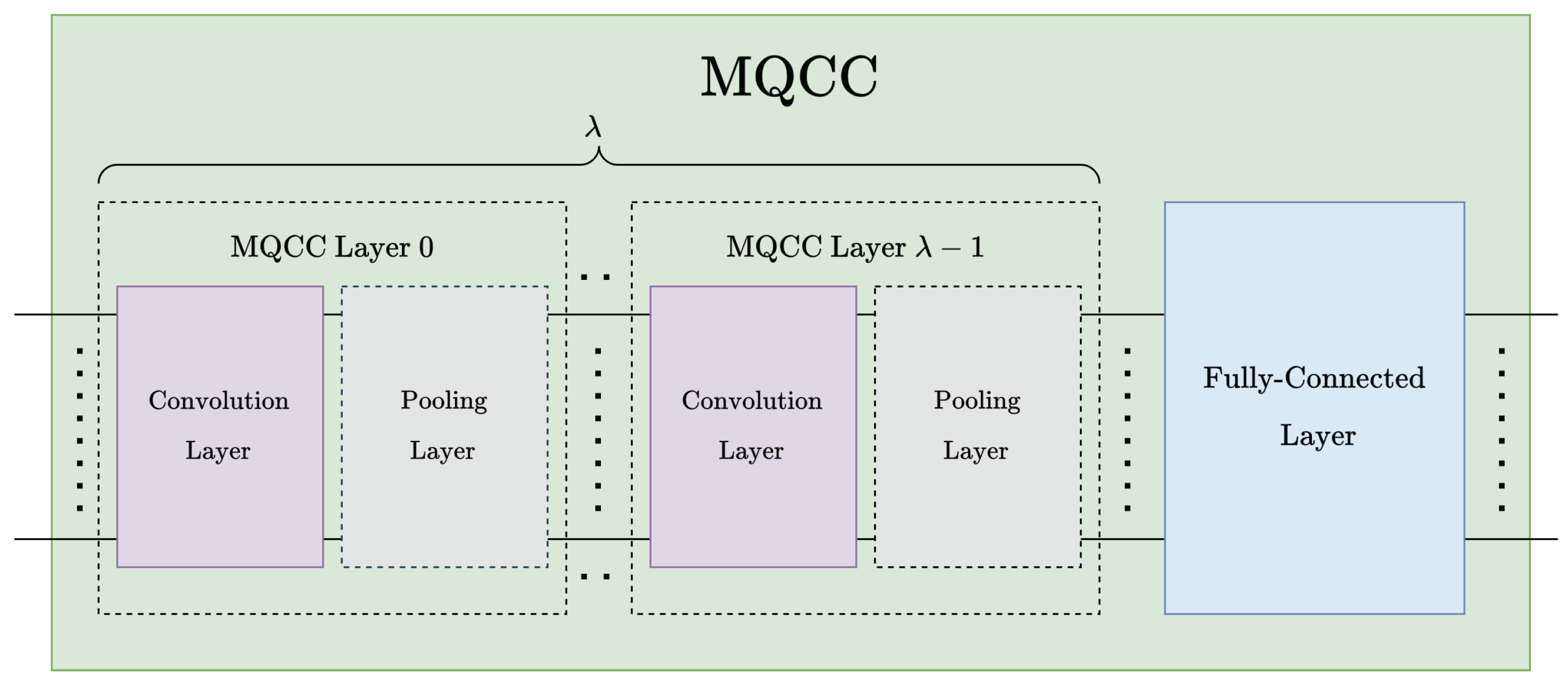
4.4. Multidimensional Quantum Convolutional Classifier

The proposed multidimensional quantum convolution classifier framework, see Figure 20, resembles cnn [2] structures. After a sequence of convolution-pooling (CP) pairs, the model is finally connected to a fully-connected layer, see Figure 15 and Figure 20. The total number of layers in the proposed model can be expressed in terms of CP pairs as

2 λ + 1

, where

λ

is the number of CP pairs.

It is worth mentioning that there is no advantage in changing the number of features among convolution/pooling layers in the mqcc because of the implementation constraints. Therefore, the total number of kernel features can be estimated globally instead of layer-by-layer.

The circuit width of mqcc (35) can be derived from the number of convolution layers, pooling layers, and the fully-connected layer. Input data is encoded using n qubits and each convolution operation adds

n_{f} = ⌈ {log}_{2} N_{F} ⌉

qubits for

N_{F}

features and

n_{k} = ⌈ {log}_{2} N_{K} ⌉

qubits per layer for kernels. In addition, the fully-connected operation contributes

n_{c} = ⌈ {log}_{2} N_{C} ⌉

qubits to encode

N_{C}

output features/classes. On the other hand, each Euclidean pooling layer frees ℓ qubits, which can then be reused by other layers.

\begin{matrix} n_{mqcc}^{Avg} & = n + n_{f} + λ n_{k} + n_{c} \\ n_{mqcc}^{Euclidean} & = n + n_{f} + n_{k} + max (0, (λ - 1) n_{k} - λ ℓ + n_{c}) \end{matrix}

(35)

The mqcc can be further parallelized in terms of circuit depth between the inter-layer convoluti- on/fully-connected layers. This parallelism can be achieved by performing (multiplexed) MAC operations from the quantum convolution and fully-connected layers in parallel with the stride operation from the previous layer(s) of quantum convolution. The circuit depth of mqcc can be derived as shown in (36).

\begin{matrix} Δ_{mqcc} & = {max}_{i = 0}^{d - 1} Δ_{U_{stride}} (n_{i}, n_{k_{i}}) + λ (Δ_{H} + Δ_{SWAP}) \\ + \sum_{j = 0}^{λ - 2} max ({max}_{i = 0}^{d - 1} Δ_{U_{stride}} (n_{i} - j ℓ_{i}, n_{k_{i}}), Δ_{U_{K}} (n_{k}, n_{f})) \\ + max (Δ_{FC} (n - (λ - 1) ℓ, n_{c}), Δ_{U_{K}} (n_{k}, n_{f})) \end{matrix}

(36)

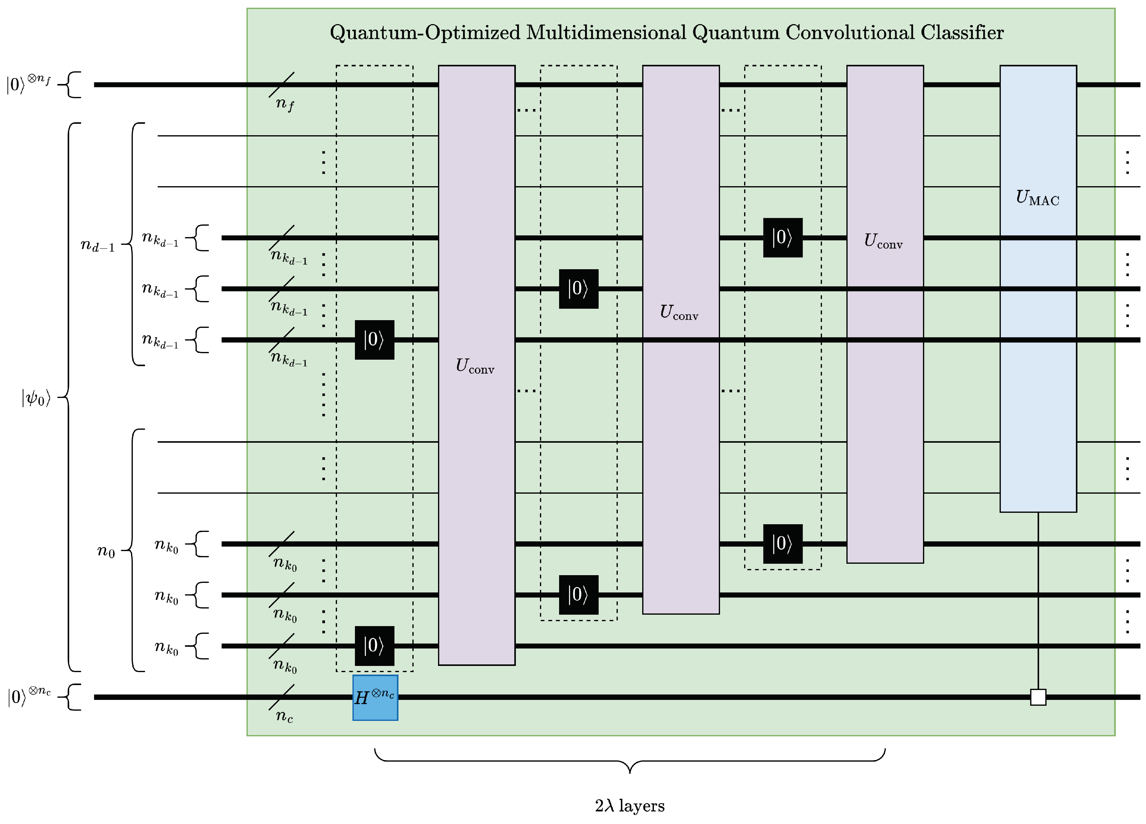
4.5. Optimized MQCC

Figure 21 presents a width-optimized implementation of MQCC, to which we refer as mqccoptimized. To reduce the required number of qubits, the convolution and pooling operations are swapped which allows kernel qubits to be trimmed for each convolution layer, see Section 4.2. To achieve higher processing efficiency, trimmed qubits are reassigned to later layers of dimension reduction and run in parallel. Furthermore, only Euclidean pooling with partial measurements is used because of the inherent circuit depth efficiency. The circuit width of mqccoptimized is shown in (37), where n is the number of qubits corresponding to the data size,

n_{f}

is the number of qubits corresponding to the features, and

n_{c}

is the number of qubits corresponding to the classes. If necessary, additional pooling operations can be applied to keep the circuit width at or below the absolute minimum number of qubits n, via excluding qubits dedicated to features and classes. It should be noted that reordering convolution and pooling operations reduces the maximum number of convolution operations by 1.

n_{bad hbox} = n + n_{f} + n_{c}

(37)

Accordingly, the depth of mqccoptimized can be expressed as shown in (38).

\begin{matrix} Δ_{mqcc}^{opt} & = {max}_{i = 0}^{d - 1} Δ_{U_{stride}} (n_{i} - ℓ_{i}, n_{k_{i}}) + λ (Δ_{H} + Δ_{SWAP}) \\ + \sum_{j = 1}^{λ - 1} max ({max}_{i = 0}^{d - 1} Δ_{U_{stride}} (n_{i} - j ℓ_{i}, n_{k_{i}}), Δ_{U_{K}} (n_{k}, n_{f})) \\ + max (Δ_{FC} (n - λ ℓ, n_{c}), Δ_{U_{K}} (n_{k}, n_{f})) \end{matrix}

(38)

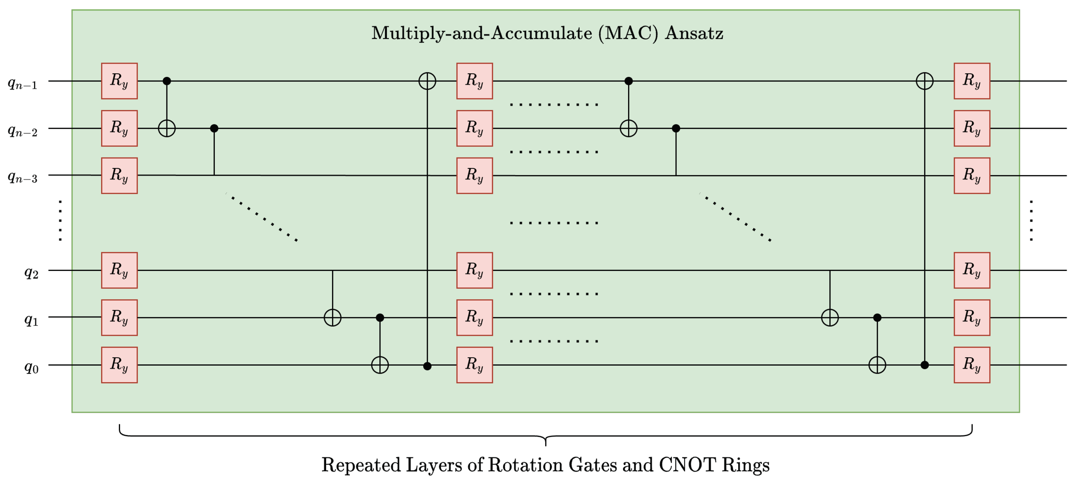
To further reduce the depth of mqccoptimized, we investigated replacing inverse-c2q operations for mac operations with different parameterized ansatz. More specifically, a common ansatz in qml, namely, NLocal operation in Qiskit [39] or

BasicEntanglerLayer in Pennylane [40] was utilized, see Figure 22. The depth of this ansatz is linear with respect to the data size, see (39), which is a significant improvement over arbitrary state synthesis, which has a circuit depth of

O (2^{n})

for an n-qubit state. Although the ansatz could potentially reduce circuit depth, its structure lacks theoretical motivation or guarantees for high fidelity when modeling convolution kernels.

Δ_{α} (n, ℓ) = ℓ \cdot n + 1

(39)

5. Experimental Work

In this section, we first detail our experimental setup, followed by the results for the proposed mqcc technique. Experiments were conducted using real-world, multidimensional image data to test both the individual and composite components of our techniques.

5.1. Experimental Setup

The mqcc methodology was validated by first evaluating its components, and then evaluating the complete technique. For experiments on 1-D data, we used audio material published by the European Broadcasting Union for sound quality assessment [41]. Using a pre-processing step, the data was converted into a single channel, with the data size varying from

2^{8}

data points to

2^{20}

data points, sampled at a rate of

44.1

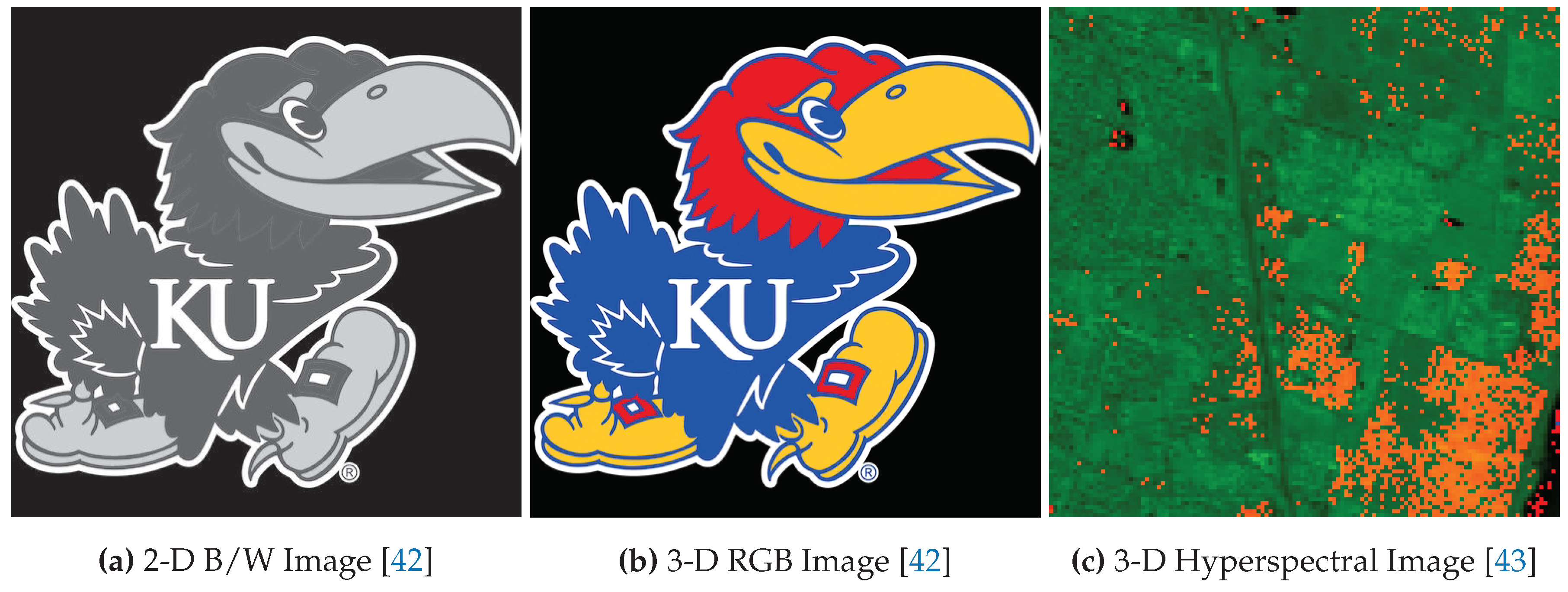
kHz. Further tests were conducted using high-resolution, multidimensional, real-world images of various kinds. The 2-D images used were either black-and-white or color Jayhawks [42], as shown in Figure 23, sized from

(8 \times 8)

pixels to

(512 \times 512 \times 3)

pixels. For the 3-D image experiments, we used hyperspectral images from the Kennedy Space Center (KSC) dataset [43]. It was pre-processed and resized, with the sizes ranging from (

8 \times 8 \times 8

) pixels to (

128 \times 128 \times 128

) pixels.

Simulations of quantum convolution operation were run using Qiskit SDK (v0.45.0) from IBM Quantum [20] over the given data. To demonstrate the effect of statistical noise on the fidelity (40), both noise-free and noisy (with 1,000,000 circuit samples/shots) simulation environments were evaluated.

Fidelity (X, Y) = \frac{〈 X, Y 〉}{X_{F} Y_{F}}

(40)

To evaluate the performance of the complete mqcc technique, it was tested against cnns, qcnn, and quanvolutional neural networks by its capabilities of binary classification on real-world datasets such as MNIST [45], FashionMNIST [46], and CIFAR10 [47]. The classical components in these trials were run using PyTorch (v2.1.0) [48], while the quantum circuits used Pennylane (v0.32.0), a Xanadu QML-focused framework [49].

The experiments were performed on a cluster node at the University of Kansas [50]. The node consisted of a 48-Core Intel Xeon Gold 6342 CPU, three NVIDIA A100 80GB GPUs (CUDA version 11.7) with PCIe 4.0 connectivity and 256GB of 3200MHz DDR4 RAM. To account for initial parameter variance in ML or noise in noisy simulations, experiments were repeated for 10 trials with the median being displayed in graphs.

5.2. Configuration of ML models

The different techniques fundamentally being ML models meant that they could share some parameters and metrics during their testing. For example, the log loss and the Adam optimizer [51] was shared by all the techniques, and the "feature-count" metric was shared between the cnn and mqcc, which had 4 features per convolution layer. The parameters that were unique to each model are discussed next.

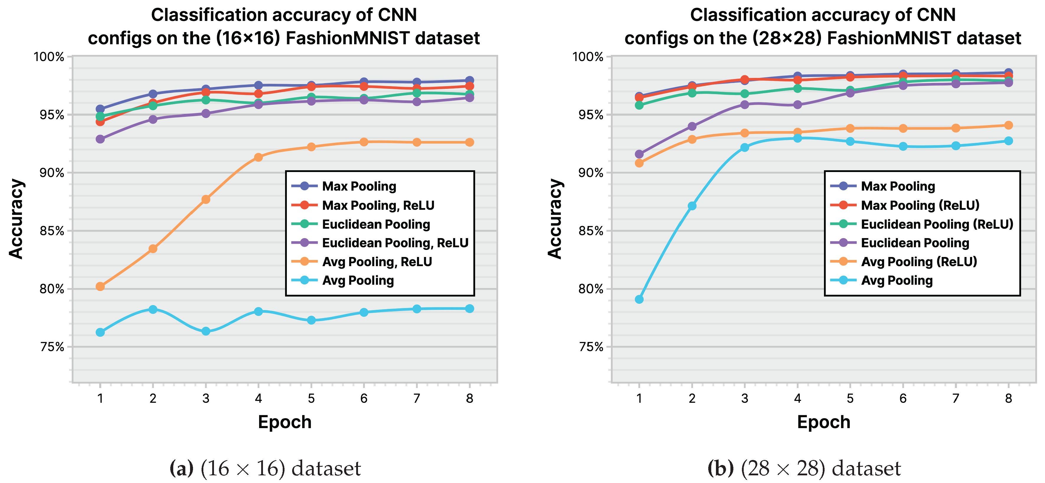
Convolutional Neural Networks: In Figure 24, we show the classification accuracy of the cnn model on (

16 \times 16

) and (

28 \times 28

) FashionMNIST datasets, using average pooling, max pooling, and Euclidean pooling. The plots show the obtained accuracy with and without ReLU [52], which is an optional layer that can be appended to each pooling layer in cnn. Based on the results, which show Max Pooling without ReLU to be the configuration with the best accuracy, we chose it to be the baseline configuration for cnn in our tests.

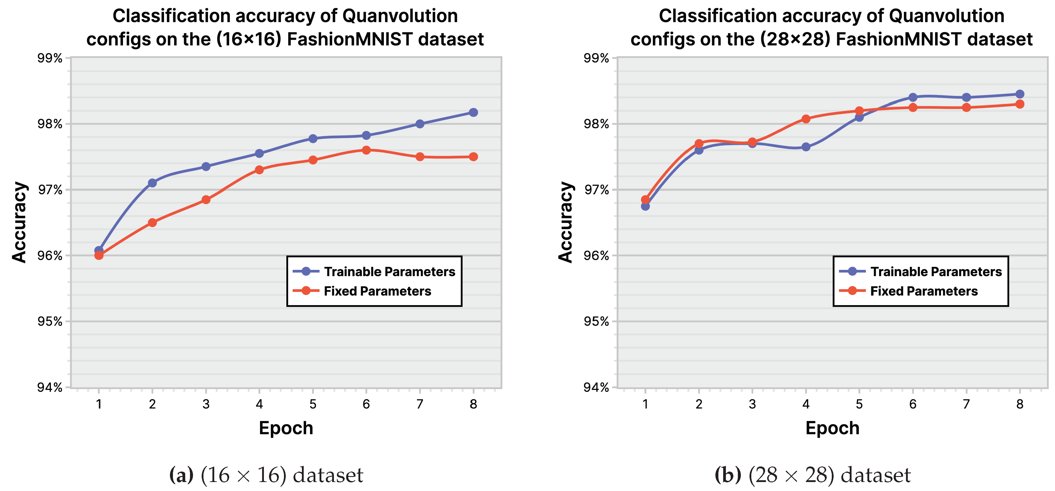
Quanvolutional Neural Networks: While quanvolutional neural networks were initially introduced without a trainable random quantum circuit in the quanvolutional layer, later work has suggested implementing parameterized and trainable quanvolutional layers. We, therefore, test both the trainable and non-trainable quanvolutional techniques and Figure 25 demonstrates that the trainable variant outperforms the other method in the (

16 \times 16

) FashionMNIST dataset, although the differences are negligible on the (

28 \times 28

) dataset. This is used as evidence behind our decision to use the trainable variant of the quanvolutional neural network as the baseline for comparison with the other models.

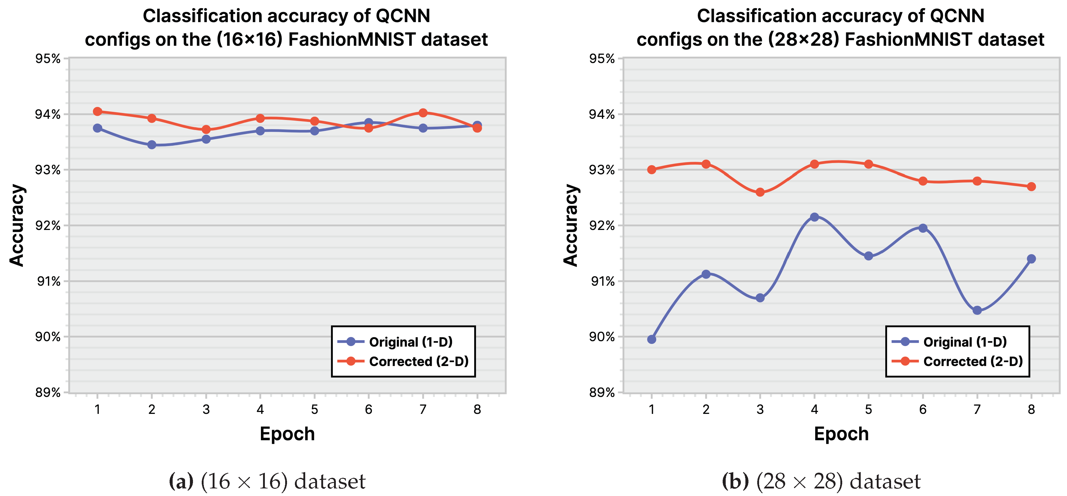
Quantum Convolutional Neural Networks: We based our implementation of qcnn on [53], however, some modifications were made to the technique to work around limitations present in the data encoding method. When encoding data that is not of size

2^{n}

in each dimension, the original method flattens (vectorizes) the input before padding with zeros, as opposed to padding each dimension. However, this sacrifices the advantage of multidimensional encoding, where each dimension is mapped to a region of qubits. To ensure a level field between qcnn and mqcc, the (

16 \times 16

) and (

28 \times 28

) FashionMNIST datasets were tested both for the original (1-D) and a corrected (2-D) data encoding configuration of qcnn, the results of which are shown in Figure 26. As expected, we see a clear improvement on the (

28 \times 28

) dataset and based on this, we chose the corrected (2-D) data encoding method as our baseline qcnn for comparison against other ML models.

5.3. Results and Analysis

We first present the results of the quantum convolution operations on data with varying dimensionalities. Then, we compare the fidelity results of the quantum convolution under a noisy simulation environment with reference to classical convolution implementation. Finally, we present the results for mqcc.

5.3.1. Quantum Convolution Results

Similar to pooling, the fidelity of the quantum convolution technique was tested in both a noise-free and noisy environment against a classical implementation using common

(3 \times 3)

and

(5 \times 5)

filter kernels. These kernels, as described in [Section 5.3.1–Section 5.3.1[, include the Averaging

F_{avg}

, Gaussian blur

F_{blur}

, Sobel edge-detection

F_{Sx}

F_{Sy}

, and Laplacian of Gaussian blur (Laplacian)

F_{L}

filters. To enable a quantum implementation of these kernels, a classical pre-processing step zero-padded each kernel until the dimensions were an integer power of two. As negative values may occur in classical convolution, the magnitudes of the output values were cast into a single-byte range

[0, 255]

in a classical post-processing step.

.35

F_{avg}^{3 \times 3} = \frac{1}{9} [\begin{matrix} 1 & 1 & 1 \\ 1 & 1 & 1 \\ 1 & 1 & 1 \end{matrix}],

(41a)

F_{avg}^{5 \times 5} = \frac{1}{25} [\begin{matrix} 1 & 1 & 1 & 1 & 1 \\ 1 & 1 & 1 & 1 & 1 \\ 1 & 1 & 1 & 1 & 1 \\ 1 & 1 & 1 & 1 & 1 \\ 1 & 1 & 1 & 1 & 1 \end{matrix}]

(41b)

.35

F_{blur}^{3 \times 3} = \frac{1}{16} [\begin{matrix} 1 & 2 & 1 \\ 2 & 4 & 2 \\ 1 & 2 & 1 \end{matrix}],

(42a)

F_{blur}^{5 \times 5} = \frac{1}{273} [\begin{matrix} 1 & 4 & 7 & 4 & 1 \\ 4 & 16 & 26 & 16 & 4 \\ 7 & 26 & 41 & 26 & 7 \\ 4 & 16 & 26 & 16 & 4 \\ 1 & 4 & 7 & 4 & 1 \end{matrix}]

(42b)

.35

F_{Sx} = \frac{1}{4} [\begin{matrix} 1 & 0 & - 1 \\ 2 & 0 & - 2 \\ 1 & 0 & - 1 \end{matrix}],

(43a)

F_{Sy} = \frac{1}{4} [\begin{matrix} 1 & 2 & 1 \\ 0 & 0 & 0 \\ - 1 & - 2 & - 1 \end{matrix}]

(43b)

.35

F_{L}^{3 \times 3} = \frac{1}{6} [\begin{matrix} 1 & 1 & 1 \\ 1 & - 8 & 1 \\ 1 & 1 & 1 \end{matrix}],

(44a)

F_{L}^{5 \times 5} = \frac{1}{20} [\begin{matrix} 1 & 1 & 1 & 1 & 1 \\ 1 & 1 & 1 & 1 & 1 \\ 1 & 1 & - 24 & 1 & 1 \\ 1 & 1 & 1 & 1 & 1 \\ 1 & 1 & 1 & 1 & 1 \end{matrix}]

(44b)

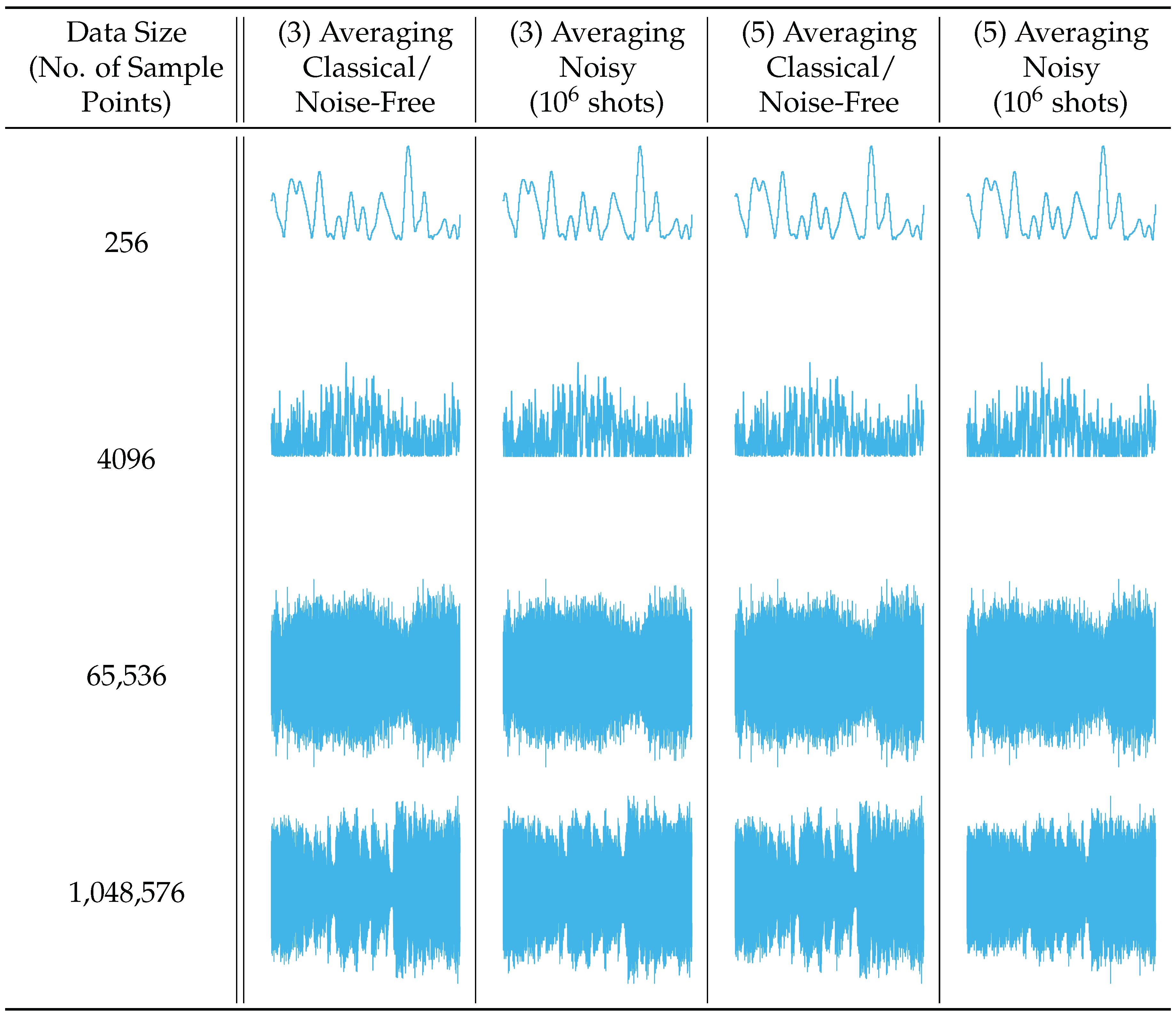
A 1-D averaging kernel of sizes (

1 \times 3

) and (

1 \times 5

) was applied to audio files after pre-processing, described in Section 5.1, with data size ranging from

2^{8}

2^{20}

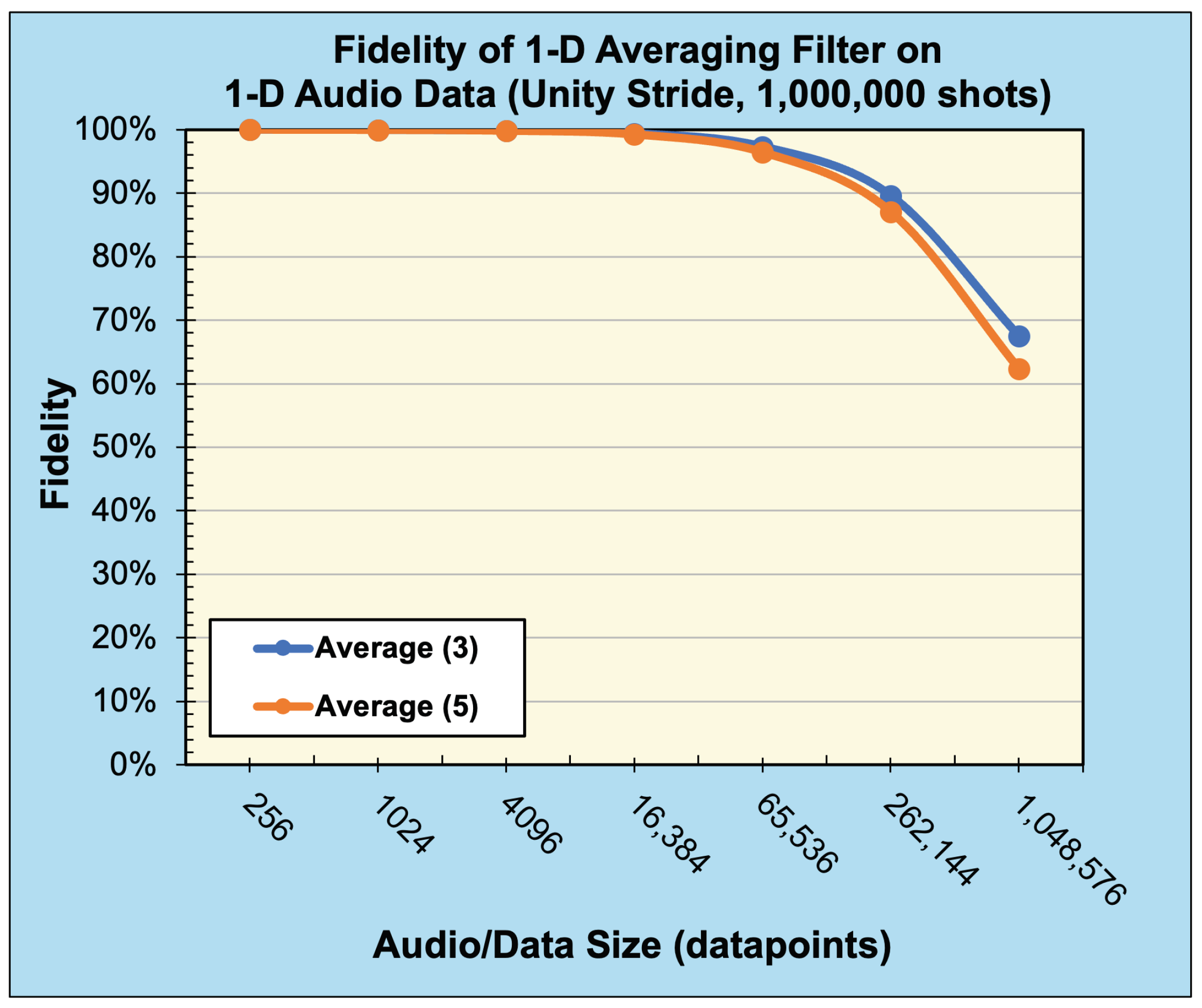
data points. Figure 27 presents the reconstructed output data of this operation, with Figure 28 displaying the associated calculated fidelity.

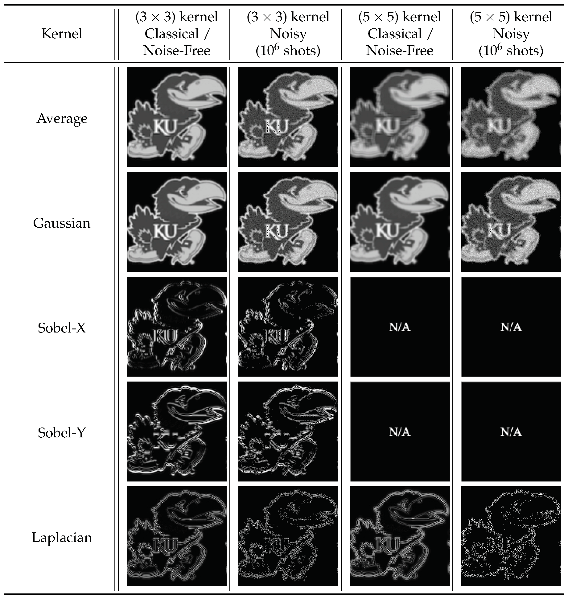
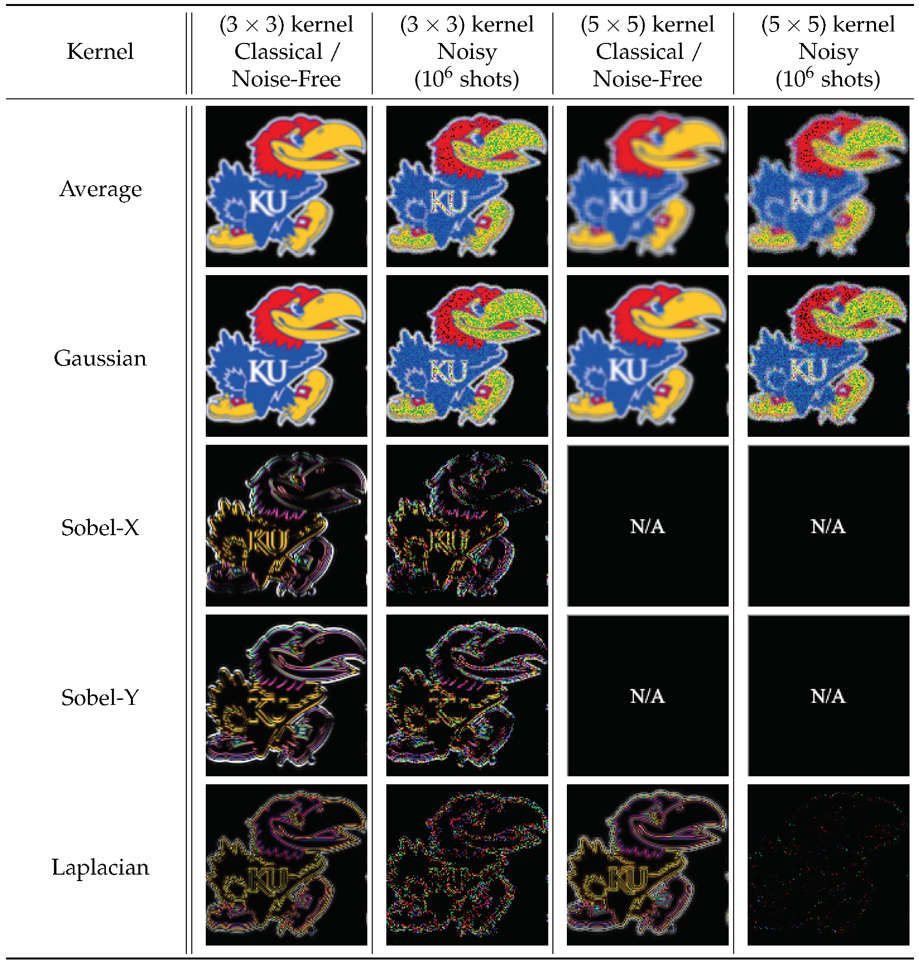
The 2-D Averaging, Gaussian blur, Sobel edge-detection, and Laplacian kernels were applied to 2-D black-and-white and 3-D RGB Jayhawk images see Figure 23, ranging from (

8 \times 8

) to (

512 \times 512

) pixels and (

8 \times 8 \times 3

) pixels to (

512 \times 512 \times 3

) pixels, respectively.

The reconstruction from convolution operations in classical, noise-free, and noisy environments on (

128 \times 128

) and (

128 \times 128 \times 3

)-pixel input images can be seen in Table 1 and Table 2, respectively.

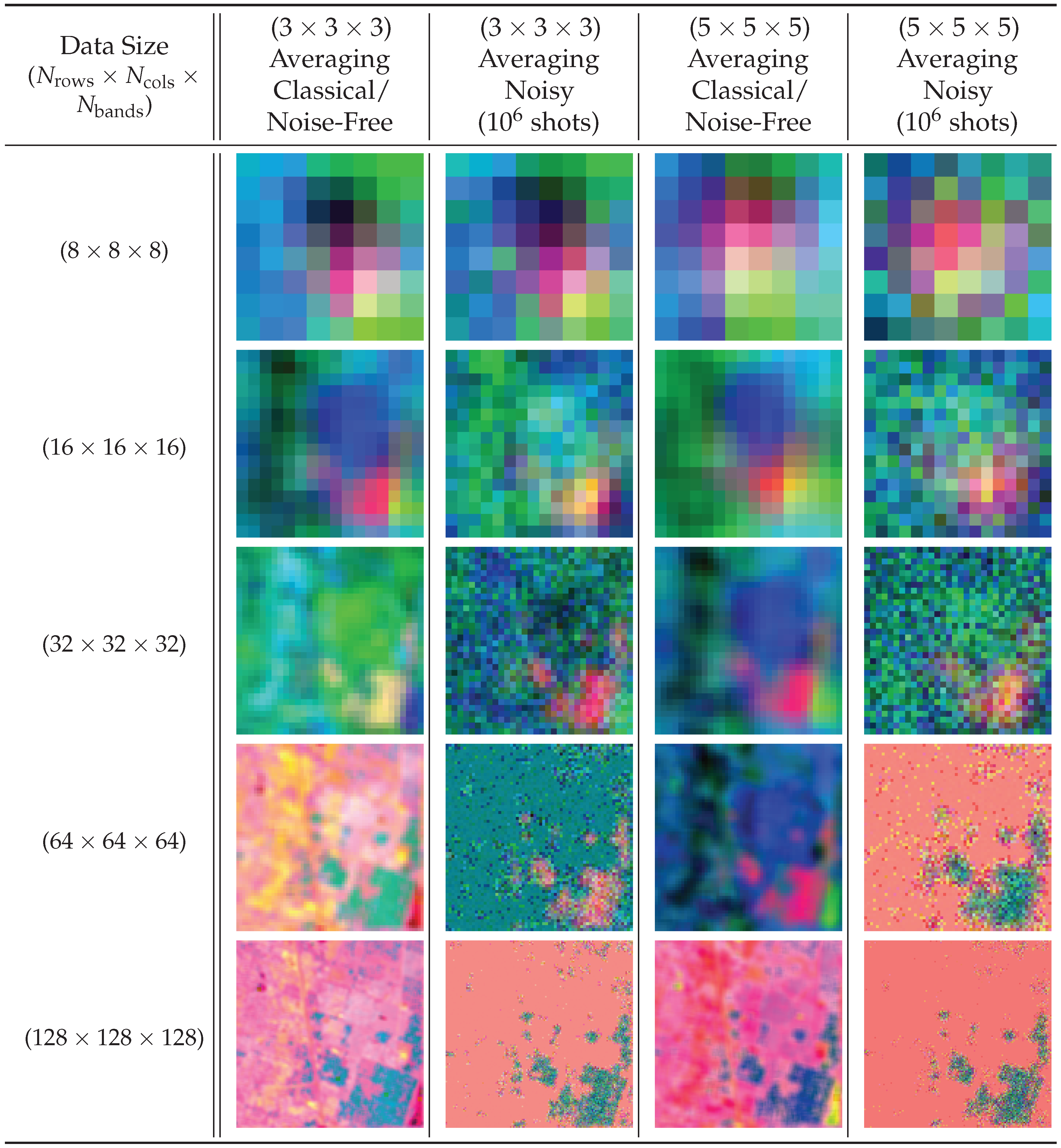
Finally, a 3-D averaging kernel of sizes (

3 \times 3 \times 3

) and (

5 \times 5 \times 5

) was applied to hyperspectral images from the KSC

dataset [43] with pre-processing applied to ensure images were resized to a power of two, ranging from (

8 \times 8 \times 8

) pixels to (

128 \times 128 \times 128

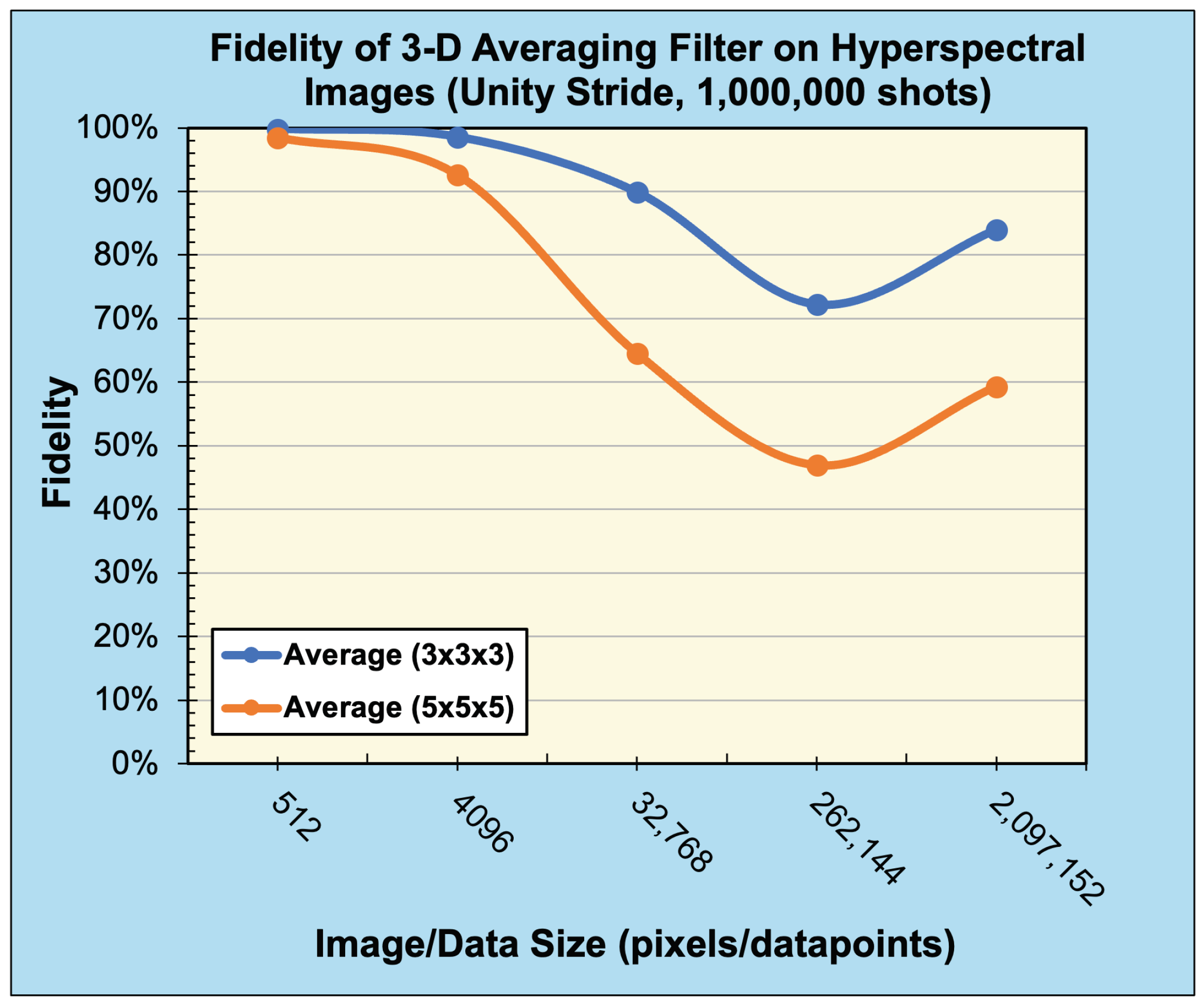
) pixels in size. Figure 29 shows the reconstructed output images, while Figure 30 illustrates the fidelity of the operation compared to its classical counterpart.

Compared to the expected, classically generated results, the noise-free quantum results tested at 100% fidelity across all trials. Therefore, in a noise-free environment, given the same inputs, the proposed convolution techniques have no degradation compared to classical convolution. The fidelity of noisy simulation using 1-D audio and 3-D hyperspectral data are presented in Figure 28 and Figure 30, respectively. The fidelity degradation in both figures is due to the statistical noise where the constant shot count (number of circuit samples) becomes less and less sufficient to describe the increasing data size.

6. Discussion

In this section, we discuss the results of our experiments with MQCC and compare them against the other models in terms of the number of required training parameters, the accuracy of the model, and circuit depth of the implemented model.

6.1. Number of parameters

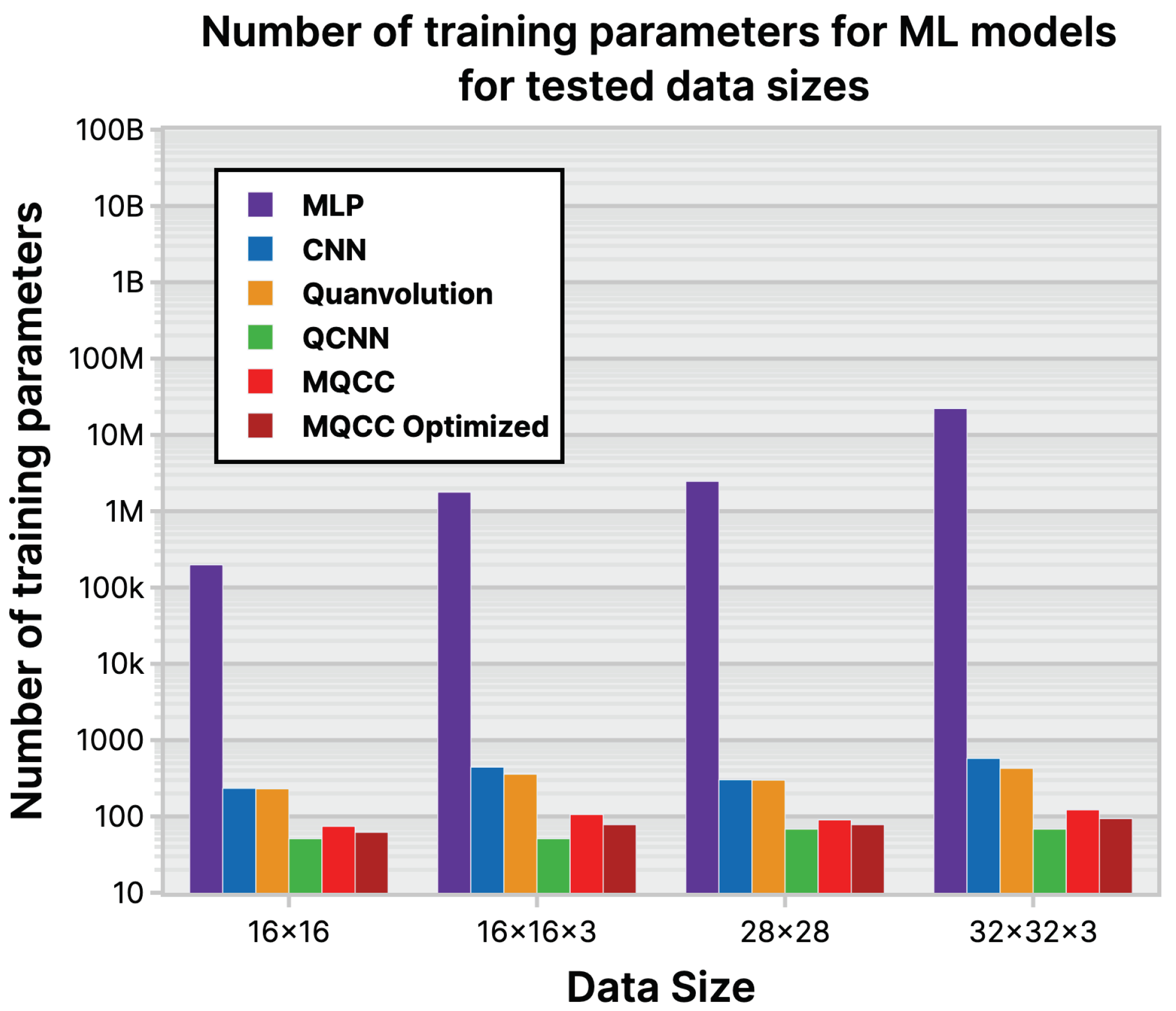
Among the ml models evaluated, mqcc had the fewest trainable parameters, see Figure 31. This implies potential advantages such as reduced memory usage and faster performance when using classical gradient descent. Although the reduction in parameter decreases from (mlp to cnn) and then further from (cnn to mqcc), parameter reduction diminishes from (mlp to cnn) and further from (cnn to mqcc), there is still a significant

83.62 %

decrease in parameter count.

6.2. Loss History and Accuracy

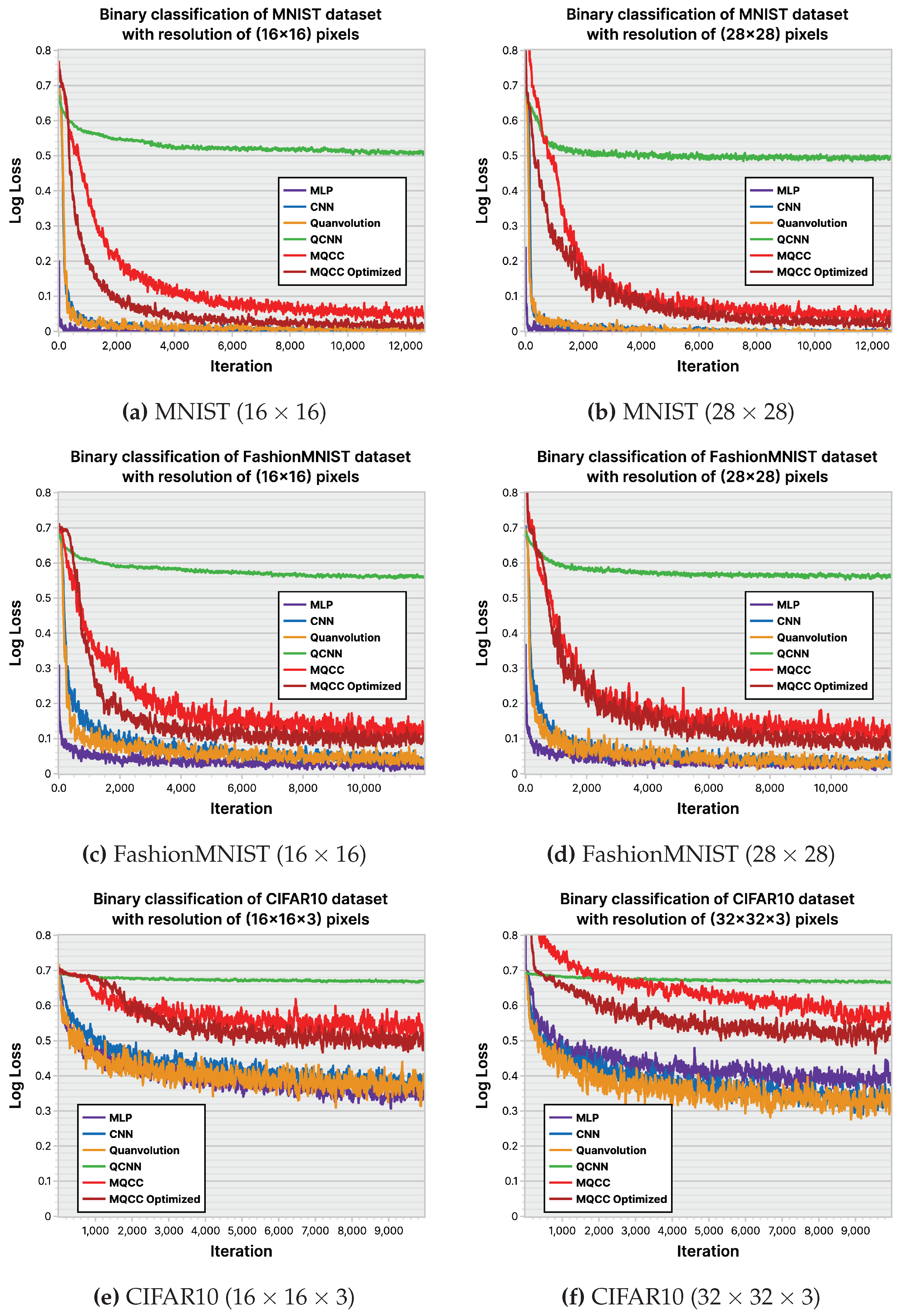
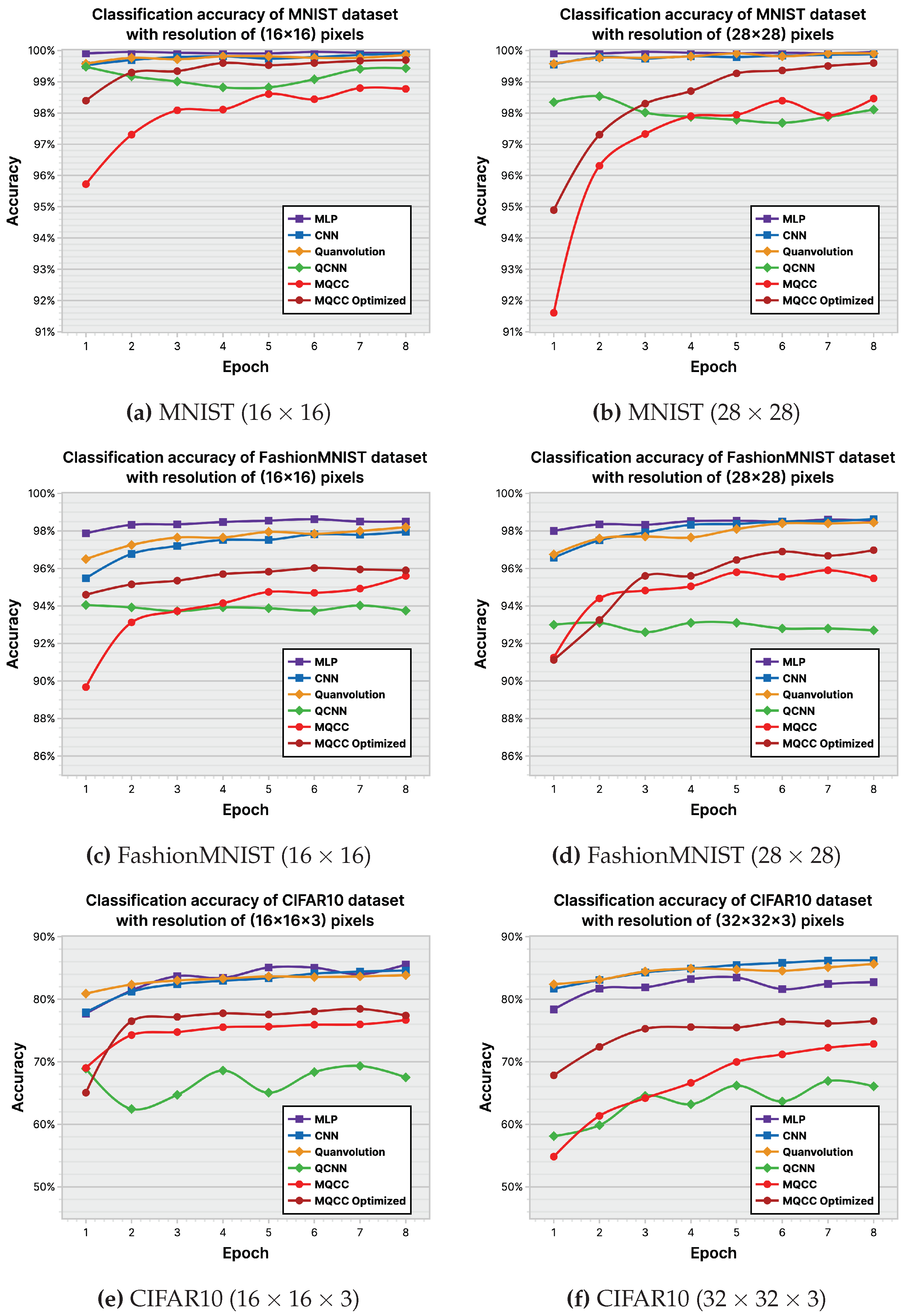
ml-based classifiers aim to maximize the accuracy of their classifications, measured by a loss function during training to estimate the accuracy that may be exhibited when deployed. Hence, Figure 32 and Figure 33 depict the performance of the ml models across the experimental datasets in their plotting of log-loss history and classification accuracy. The MNIST [45] dataset is not complex enough to effectively distinguish models, however, differences begin to emerge in the FashionMNIST [46] and CIFAR10 [47] datasets. mlp consistently achieves the highest accuracy across trials due to its larger parameter count, allowing for greater flexibility in adapting to nuances in input. cnn showcases its ability to select relevant input features using convolution and data locality, demonstrating the second-highest accuracy. Among the tested models, qcnn generally performs the poorest, displaying its inability to properly leverage data locality. However, comparing the accuracy of mqcc and quanvolutional neural networks is inconclusive. Quanvolutional neural networks performed better on FashionMNIST, whereas mqcc performed better on CIFAR10.

6.3. Gate Count and Circuit Depth

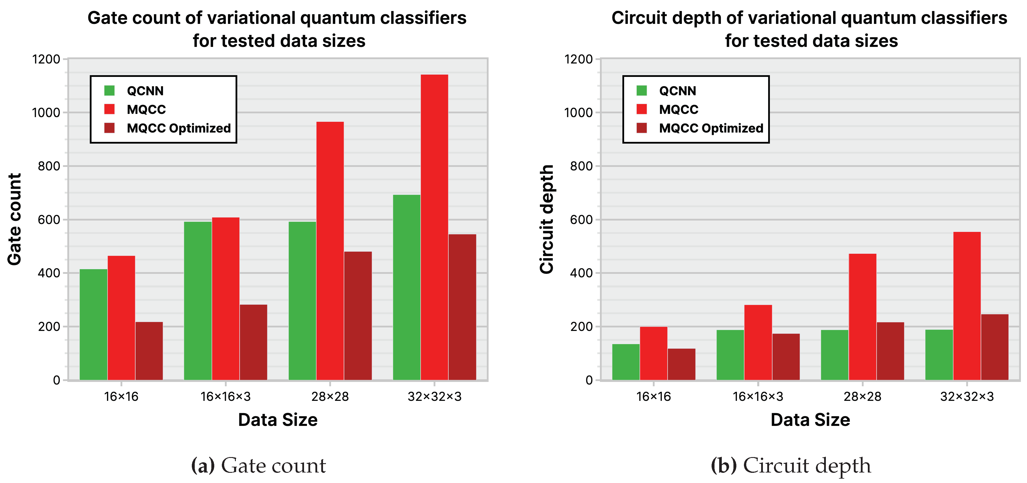
Although comparing mqcc, mqccoptimized, and qcnn with quantum metrics like gate count and circuit depth is viable, see Figure 34, it is challenging to include quanvolutional neural networks in the comparison due to their significant differences from the other models. These differences are due to the quantum component within quanvolutional neural networks constituting a small fraction of the entire algorithm, bringing it closer to a classical algorithm than a quantum algorithm. Meanwhile, comparing the techniques of mqcc and qcnn in Figure 34, highlights the rationale behind developing mqccoptimized. Initially, mqcc performed worse than qcnn in gate count and circuit depth. However, after optimizations, mqcc matches the performance of qcnn and even outperforms it in best-case scenarios. While the qcnn architecture appears more suitable for shallower quantum circuits than mqcc, it is because the high parallelization of each qcnn layer halves the active qubits. Despite qcnn using half the active qubits per layer than mqcc, mqcc utilizes the extra qubits for weights and features, with each pooling layer reducing the qubit count by a constant amount,

n_{k}

. However, as qcnn’s structure was motivated by the classical convolution operation, they usually need more complex and deeper “convolution” and “pooling” ansatz to attain a higher accuracy.

7. Conclusions

In this paper, we presented the multidimensional quantum convolutional classifier (MQCC) that consists of quantum convolution, quantum pooling, and a quantum fully-connected layer. We leveraged existing convolution techniques to support multiple features/kernels and utilized it in our proposed method. Furthermore, we proposed a novel width-optimized quantum circuit that reuses freed-up qubits from pooling layer in the subsequent convolutional layer. The proposed MQCC additionally preserves data locality in the input data which has shown to improve data classification in convolutional classifiers. The MQCC methodology is generalizable for any arbitrary multidimensional filter operation and pertinent for multi-feature extraction. The proposed method can also support data of arbitrary dimensionality since the underlying quantum pooling and convolution operations are generalizable across data dimensions. We experimentally evaluated the proposed MQCC on various real-world multidimensional images, utilizing several filters through simulations on state-of-the-art quantum simulators from IBM Quantum and Xanadu. In our experiments, MQCC produced higher classification accuracy while having a lower training time and reduced quantum gate count. In our future work, we are planning on expanding mqcc with additional convolution capabilities such as arbitrary striding and dilation and further optimizing it for deployment on real-world quantum processors. In addition, we will investigate using our proposed quantum techniques for real-life applications such as medical imaging and classification.

Author Contributions

Conceptualization: E.E., M.J., D.K., and V.J.; Methodology: E.E., M.J., D.K., and V.J.; Software: E.E., M.J., D.K., and D.L.; Validation: E.E., M.J., V.J., A.N., D.K., and D.L.; Formal analysis: E.E., M.J., D.L., D.K., and V.J.; Investigation: E.E., M.J., V.J., A.N., D.K., D.L., I.I., M.C., A.F., E.V., M.S., A.A., and E.B.; Resources: E.E., M.J., A.N., D.L., V.J., M.C., D.K., A.F., I.I., E.B., M.S., A.A., and E.V.; Data curation: E.E., M.J., V.J., A.N., D.K., D.L., I.I., M.C., A.F., E.V., M.S., E.B., and A.A.; Writing—original draft preparation: E.E., A.N., M.J., V.J., D.K., D.L., I.I., and M.C.; Writing—review and editing: E.E., M.J., V.J., A.N., D.K., D.L., I.I., M.C., A.F., E.V., M.S., E.B., and A.A.; Visualization: E.E., M.J., V.J., A.N., D.K., D.L., I.I., M.C., A.F., E.V., M.S., E.B., and A.A.; Supervision: E.E.; Project administration: E.E.; Funding acquisition: E.E. All authors have read and agreed to the published version of the manuscript.

Funding

This research received no external funding.

Data Availability Statement

The audio samples used in this work are publicly available from the European Broadcasting Union at https://tech.ebu.ch/publications/sqamcd (accessed on 23 February 2024) as file 64.flac [41]. The hyperspectral data used in this work are publicly available from the Grupo de Inteligencia Computacional (GIC) at https://www.ehu.eus/ccwintco/index.php/Hyperspectral_Remote_Sensing_Scenes#Kennedy_Space_Center_(KSC) (accessed on 23 February 2024) under the heading Kennedy Space Center (KSC) [43].

Acknowledgments

This research used resources of the Oak Ridge Leadership Computing Facility, which is a DOE Office of Science User Facility supported under Contract DE-AC05-00OR22725.

Conflicts of Interest

The authors declare no conflicts of interest.

Abbreviations

References

Villalobos, P.; Sevilla, J.; Besiroglu, T.; Heim, L.; Ho, A.; Hobbhahn, M. Machine learning model sizes and the parameter gap. arXiv 2022, arXiv:2207.02852, preprint. [Google Scholar]
LeCun, Y.; Kavukcuoglu, K.; Farabet, C. Convolutional networks and applications in vision. In Proceedings of the 2010 IEEE International Symposium on Circuits and Systems, Paris, France, NY, USA, 2010, 30 May–2 June 2010; IEEE: New York; pp. 253–256. [Google Scholar]
LeCun, Y.; Bengio, Y.; Hinton, G. Deep learning. Nature 2015, 521, 436–444. [Google Scholar] [CrossRef] [PubMed]
Chakraborty, S.; Dey, L. Computing for Data Analysis: Theory and Practices; Springer Nature Singapore 2023, pp. 161–178.
Peruzzo, A.; McClean, J.; Shadbolt, P.; Yung, M.H.; Zhou, X.Q.; Love, P.J.; Aspuru-Guzik, A.; O’Brien, J.L. A variational eigenvalue solver on a photonic quantum processor. Nature Commun. 2014, 5, 4213. [Google Scholar] [CrossRef]
Havlíček, V.; Córcoles, D. and Temme, K.; Harrow, W.; Kandala, A.; Chow, J.; Gambetta, M. Supervised learning with quantum-enhanced feature spaces. Nature 2019, 567, 209–212. [Google Scholar] [CrossRef] [PubMed]
Farhi, E.; Goldstone, J.; Gutmann, S. A quantum approximate optimization algorithm. arXiv 2014, arXiv:1411.4028, preprint. [Google Scholar]
Farhi, E.; Neven, H. Classification with quantum neural networks on near term processors. arXiv 2018, arXiv:1802.06002, preprint. [Google Scholar]
Schuld, M.; Bocharov, A.; Svore, M. and Wiebe, N. Circuit-centric quantum classifiers. Physical Review A 2020, 101, 032308. [Google Scholar] [CrossRef]
Anton, F. K.; Franco, N. Quantum Bits with Josephson Junctions; Springer, Cham. 2019.
Williams, C.P. ; Explorations in Quantum Computing; 2nd edition: Springer-Verlag London Limited 2011.
Shende, V.; Bullock, S.; Markov, I. Synthesis of quantum-logic circuits. IEEE Trans. Comput. Aided Des. Integr. Circuits Syst. 2006, 25, 1000–1010. [Google Scholar] [CrossRef]
Balauca, S.; Arusoaie, A. Efficient Constructions for Simulating Multi Controlled Quantum Gates. Computational Science – ICCS, 22nd International Conference, London, UK, June 21–23, 2022, 25, 179–194 Springer International Publishing. [Google Scholar] [CrossRef]
Jeng, M.; Islam, S.I.U.; Levy, D.; Riachi, A.; Chaudhary, M.; Nobel, M.A.I.; Kneidel, D.; Jha, V.; Bauer, J.; Maurya, A.; Mahmud, N.; El-Araby, E. Improving quantum-to-classical data decoding using optimized quantum wavelet transform. J. Supercomput. 2023, 79, 20532–20561. [Google Scholar] [CrossRef]
Jeng, M.; Nobel, A.; Jha, V.; Levy, D.; Kneidel, D.; Chaudhary, M. and Islam, I.; Rahman, M.; El-Araby, E. Generalized Quantum Convolution for Multidimensional Data. Entropy 2023, 25, 11. [Google Scholar] [CrossRef] [PubMed]
Yao, X.; Wang, H.; Liao, Z.; Chen, M.; Pan, J.; Li, J.; Zhang, K.; Lin, X.; Wang, Z.; Luo, Z.; Zheng, W.; Li, J.; Zhao, M.; Peng, X.; Suter, D. Quantum Image Processing and Its Application to Edge Detection: Theory and Experiment. Phys. Rev. X 2017, 7, 031041. [Google Scholar] [CrossRef]
Li, X. and Yang, G. and Torres, M.; Zheng, D.; Wang, L. A Class of Efficient Quantum Incrementer Gates for Quantum Circuit Synthesis. International Journal of Modern Physics B 2014, 2. [Google Scholar] [CrossRef]
Fan, P.; Zhou, R.; Hu, W.; Jing, N. Quantum image edge extraction based on classical Sobel operator for NEQR. Quantum Information Processing 2018, 1. [Google Scholar] [CrossRef]
El-Araby, E.; Mahmud, N.; Jeng, M.J.; MacGillivray, A.; Chaudhary, M.; Nobel, M.A.I.; Islam, S.I.U.; Levy, D.; Kneidel, D.; Watson, M.R.; Jack, B.; Andrew, R. Towards Complete and Scalable Emulation of Quantum Algorithms on High-Performance Reconfigurable Computers. IEEE Trans. Comput. 2023, 72, 2350–2364. [Google Scholar] [CrossRef]
IBM Quantum. Qiskit: An Open-source Framework for Quantum Computing. Zenodo, online. [CrossRef]
Nation, P. How to measure and reset a qubit in the middle of a circuit execution. 2021. Available online: https://www.ibm.com/quantum/blog/quantum-mid-circuit-measurement (accessed on 26 February 2024).
Mi, A.; Deng, S.; Szefer, J. Securing Reset Operations in NISQ Quantum Computers. Proceedings of the 2022 ACM SIGSAC Conference on Computer and Communications Security 2022, 2279–2293. [Google Scholar]
Mahmud, N.; Jeng, M.; Nobel, Md. Alvir I.; Chaudhary, M.; Ul Islam, S M I.; Levy, D.; El-Araby, E. Efficient Data Encoding and Decoding for Quantum Computing. 2022 IEEE International Conference on Quantum Computing and Engineering (QCE), Broomfield, CO, USA, –23, 2022, 765–768. 18 September. [CrossRef]
Le, Q.; Dong, F.; Hirota, K. A flexible representation of quantum images for polynomial preparation, image compression, and processing operations. Quantum Information Processing. [CrossRef]
Zhang, Y.; Lu, K.; Gao, Y.; Wang, M. NEQR: a novel enhanced quantum representation of digital images. Quantum Information Processing, 2833. [Google Scholar] [CrossRef]
Burrus, C.S. S. ; Parks, Thomas W. DFT/FFT and Convolution Algorithms: Theory and Implementation, 1991. [Google Scholar]
Podlozhnyuk, V.; FFT-based 2D convolution. NVIDIA 2007. Available online: https://developer.download.nvidia.com/compute/cuda/1.1-Beta/x86_64_website/projects/convolutionFFT2D/doc/convolutionFFT2D.pdf (accessed on 18 February 2024).
NVIDIA. CUTLASS Convolution. Github 2023. Available online: https://github.com/NVIDIA/cutlass/blob/main/media/docs/implicit_gemm_convolution.md (accessed on 18 February 2024).
NVIDIA. Convolution Algorithms. Github 2023. Available online: https://docs.nvidia.com/deeplearning/performance/dl-performance-convolutional/index.html#conv-algo (accessed on 18 February 2024).
Ma, Y.; Ma, H.; Chu, P. Demonstration of Quantum Image Edge Extration Enhancement Through Improved Sobel Operator. IEEE Access, 2102. [Google Scholar] [CrossRef]
Zhang, Y.; Lu, K.; Gao, Y. QSobel: A novel quantum image edge extraction algorithm. Science China Information Sciences. [CrossRef]
Zhou, R.; Yu, H.; Cheng, Y.; Li, F. Quantum image edge extraction based on improved Prewitt operator. Quantum Information Processing. [CrossRef]
Li, P. Quantum implementation of the classical Canny edge detector. Multimedia Tools and Applications, 1166. [Google Scholar] [CrossRef]
Cong, I.; Choi, S.; Lukin, M.D. Quantum convolutional neural networks. Nature Phys. 2019, 15, 1273–1278. [Google Scholar] [CrossRef]
Henderson, M.; Shakya, S.; Pradhan, S.; Cook, T. Quanvolutional neural networks: powering image recognition with quantum circuits. Quantum Machine Intelligence 2020, 2, 2. [Google Scholar] [CrossRef]
Bieder, F.; Sandkühler, R.; Cattin, P. Comparison of methods generalizing max-and average-pooling. arXiv, 2: arXiv, 2103. [Google Scholar] [CrossRef]
Jeng, M.; Nobel, A.; Jha, V.; Levy, D.; Kneidel, D.; Chaudhary, M.; Islam, I.; Baumgartner, E.; Vanderhoof, E.; Facer, A.; Singh, M.; Arshad, A.; El-Araby, E. Optimizing Multidimensional Pooling for Variational Quantum Algorithms. Algorithms 2024, 17, 82. [Google Scholar] [CrossRef]
PyTorch. torch.nn.LPPool1d [Computer Software]. 2023. Available online: https://pytorch.org/docs/stable/generated/torch.nn.LPPool1d.html (accessed on 18 February 2024).
IBM Quantum. qiskit.circuit.library.NLocal [Computer Software]. 2023. Available online: https://qiskit.org/documentation/stubs/qiskit.circuit.library.NLocal.html (accessed on 18 February 2024).
Xanadu. qml.BasicEntanglerLayers [computer software]. 2023. Available online: https://docs.pennylane.ai/en/stable/code/api/pennylane.BasicEntanglerLayers.html (accessed on 18 February 2024).
Geneva, S. Sound Quality Assessment Material: Recordings for Subjective Tests. Available online: https://tech.ebu.ch/publications/sqamcd, 1988. (accessed on 18 February 2024).
Brand Center, University of Kansas. Jayhawk Images. Available online: https://brand.ku.edu/ (accessed on 18 February 2024).
Graña, M.; Veganzons, M.A.; Ayerdi, B. Hyperspectral Remote Sensing Scenes. Available online: https:// www.ehu.eus/ccwintco/index.php/Hyperspectral_Remote_Sensing_Scenes#Kennedy_Space_Center_(KSC) (accessed on 18 February 2024).
Jeng, M.; Nobel, M.A.I.; Jha, V.; Levy, D.; Kneidel, D.; Chaudhary, M.; Islam, S.I.U.; El-Araby, E. Multidimensional Quantum Convolution with Arbitrary Filtering and Unity Stride. In Proceedings of the IEEE International Conference on Quantum Computing and Engineering (QCE23), Bellevue, WA, USA, 17–22 September 2023. [Google Scholar]
Deng, L. The MNIST database of handwritten digit images for machine learning research. IEEE Signal Processing Magazine; IEEE, 2012, 29, 141–142. [Google Scholar] [CrossRef]
Xiao, H.; Rasul, K.; Vollgraf, R. Fashion-MNIST: a Novel Image Dataset for Benchmarking Machine Learning Algorithms. arXiv 2017. [Google Scholar] [CrossRef]
Krizhevsky, A. Learning Multiple Layers of Features from Tiny Images. 2009. https://www.cs.toronto.edu/~kriz/learning-features-2009-TR.pdf. (accessed on 18 February 2024).
Paszke, A.; Gross, S.; Massa, F.; Lerer, A.; Bradbury, J.; Chanan, G.; Killeen, T.; Lin, Z.; Gimelshein, N.; Antiga, L.; Desmaison, A.; Köpf, A.; Yang, E.; DeVito, Z.; Raison, M.; Tejani, A.; Chilamkurthy, S.; Steiner, B.; Fang, L.; Bai, J.; Chintala, S. Pytorch: An imperative style, high-performance deep learning library. Advances in neural information processing systems, /: https, 5555. [Google Scholar]
Bergholm, V.; Izaac, J.; Schuld, M.; Gogolin, C.; Ahmed, S.; Ajith, V.; Alam, M.S.; Alonso-Linaje, G.; AkashNarayanan, B.; Asadi, A.; Arrazola, J.M.; PennyLane: Automatic differentiation of hybrid quantum-classical computations. arXiv 2022. Available online: https://pennylane.ai/ (accessed on 18 February 2024).
KU Community Cluster, Center for Research Computing, University of Kansas. Available online: https://crc.ku.edu/systems-services/ku-community-cluster (accessed on 18 February 2024).
Kingma, D. P.; Ba, J. Adam: A method for stochastic optimization. arxiv 2014, arXiv:1412.6980. [Google Scholar]
Arora, R.; Basu, A.; Mianjy, P.; Mukherjee, A. Understanding deep neural networks with rectified linear units. arxiv 2014, arXiv:1611.01491. [Google Scholar]
Hur, T.; Kim, L.; Park, D. Quantum convolutional neural network for classical data classification. Quantum Machine Intelligence, Springer. [CrossRef]

Figure 1. The Bloch Sphere.

Figure 2. Hadamard gate diagram

Figure 3. Example parallel operation notation.

Figure 4. Controlled-NOT gate diagram.

Figure 5. Controlled-U gate diagram.

Figure 6. The square box notation for a quantum multiplexer. [12]

Figure 7. Swap gate diagram and decomposition.

Figure 8. Quantum Perfect-Shuffle Permutations. [14]

Figure 9. Quantum incrementer, decrementer, and construction of quantum shift operation.

Figure 10. Full quantum state measurement diagram.

Figure 11. Reset gate and equivalent circuit.

Figure 12. The quantum circuit for classical-to-quantum (C2Q) arbitrary state synthesis. [23]

Figure 13. Quantum multiply-and-accumulate (MAC) operation using inverse arbitrary state synthesis.

Figure 14. Quantum fully-connected layer with an

N_{out}

-feature output.

Figure 14. Quantum fully-connected layer with an

N_{out}

-feature output.

Figure 15. Decomposed and simplified quantum fully-connected layer.

Figure 16. One-dimensional quantum convolution circuit.

Figure 17. Multi-dimensional quantum convolution circuit

Figure 18. Quantum Haar Transform Circuits.

Figure 19. Multilevel, d-D Euclidean pooling circuit.

Figure 20. High-level overview of mqcc architecture.

Figure 21. Quantum-Optimized Multidimensional Quantum Convolutional Classifier (MQCC Optimized).

Figure 22. Alternate ansatz option, distinct from

U_{mac}

Figure 22. Alternate ansatz option, distinct from

U_{mac}

Figure 23. High-resolution, multidimensional, real-world input data used in experimental trials.

Figure 24. Classification accuracy of Convolutional Neural Network (cnn) configurations on the FashionMNIST dataset.

Figure 25. Classification accuracy of Quanvolution Neural Network configurations on the FashionMNIST dataset.

Figure 26. Classification accuracy of Quantum Convolutional Neural Network (qcnn) configurations on the FashionMNIST dataset,

Figure 27. The 1-D convolution (averaging) filters applied to 1-D audio samples [41].

Figure 28. Fidelity of 1-D convolution (averaging) filters with unity stride on 1-D audio data (sampled with 1,000,000 shots).

Figure 29. The 3-D convolution (averaging) filters applied to 3-D hyperspectral images (bands 0, 1, and 2) [43].

Figure 30. Fidelity of 3-D convolution (averaging) filters with unity stride on 3-D hyperspectral data (sampled with 1,000,000 shots).

Figure 31. Number of training parameters for ml models for tested data sizes

Figure 32. Loss history of ml models on various datasets.

Figure 33. Classification accuracy of ml models on various datasets.

Figure 34. Gate count and circuit depth of mqcc vs qcnn.

Table 1. 2D convolution kernels applied to a (

128 \times 128

) bw image [42].

Table 1. 2D convolution kernels applied to a (

128 \times 128

) bw image [42].

Table 2. 2D convolution kernels applied to a (

128 \times 128 \times 3

) rgb image [42].

Table 2. 2D convolution kernels applied to a (

128 \times 128 \times 3

) rgb image [42].

Disclaimer/Publisher’s Note: The statements, opinions and data contained in all publications are solely those of the individual author(s) and contributor(s) and not of MDPI and/or the editor(s). MDPI and/or the editor(s) disclaim responsibility for any injury to people or property resulting from any ideas, methods, instructions or products referred to in the content.

© 2024 by the authors. Licensee MDPI, Basel, Switzerland. This article is an open access article distributed under the terms and conditions of the Creative Commons Attribution (CC BY) license (https://creativecommons.org/licenses/by/4.0/).

Copyright: This open access article is published under a Creative Commons CC BY 4.0 license, which permit the free download, distribution, and reuse, provided that the author and preprint are cited in any reuse.

MDPI Initiatives

Important Links

Choose an area of interest and we will send you notifications of new preprints at your preferred frequency.

Disclaimer

Leveraging Data Locality in Quantum Convolutional Classifiers

Abstract

1. Introduction

2. Background

2.1. Quantum Bits and States

2.2. Quantum Gates

2.2.1. Rotation Gates

2.2.2. Hadamard Gate

2.2.3. cnot Gate

2.2.4. SWAP Gate

2.2.5. Quantum Perfect-Shuffle Permutation (PSP)

2.2.6. Quantum Shift Operation

2.3. Quantum Measurement and Reset

2.4. Classical-to-Quantum (C2Q)

2.5. Quantum Machine Learning with Variational Algorithms

3. Related Work

3.1. Data Encoding

3.2. Convolution

3.2.0.1. Classical Convolution

3.2.0.2. Quantum Convolution

3.3. Quantum Machine Learning

3.3.1. Quantum Convolutional Neural Networks

3.3.2. Quanvolutional Neural Networks

4. Materials and Methods

4.1. Quantum Fully-Connected Layer

4.1.1. Single-Feature Output

4.1.2. Multi-Feature Output

4.1.2.1. Replication:

4.1.2.2. Applying the U FC Filter:

4.1.2.3. Data Rearrangement:

4.1.3. Circuit Depth of the Quantum Fully-Connected Layer

4.2. Generalized Quantum Convolution

4.2.0.1. Stride:

4.2.0.2. Multiply-and-Accumulate (MAC):

4.2.0.3. Data Rearrangement:

4.2.1. One-Dimensional Multi-Feature Quantum Convolution

4.2.2. Multi-Dimensional Multi-Feature Quantum Convolution

4.3. Quantum Pooling

4.3.1. Quantum Average Pooling using Quantum Haar Transform

4.3.1.1. Haar Wavelet Operation:

4.3.1.2. Data Rearrangement:

4.3.2. Quantum Euclidean Pooling using Partial Measurement

4.4. Multidimensional Quantum Convolutional Classifier

4.5. Optimized MQCC

5. Experimental Work

5.1. Experimental Setup

5.2. Configuration of ML models

5.3. Results and Analysis

5.3.1. Quantum Convolution Results

6. Discussion

6.1. Number of parameters

6.2. Loss History and Accuracy

6.3. Gate Count and Circuit Depth

7. Conclusions

Author Contributions

Funding

Data Availability Statement

Acknowledgments

Conflicts of Interest

Abbreviations

References

MDPI Initiatives

Important Links

Subscribe

4.1.2.2. Applying the $U_{FC}$ Filter: