1. Introduction
Large volumes of spatiotemporal (ST) data are collected in several application domains, such as social media, healthcare, agriculture, transportation, and climate science. In this section, we briefly describe the different types of ST data, ways of analyzing ST data, the motivation for analyzing ST data in different application domains and how to model ’event’ type ST data. Machine learning, including deep learning, has been effective in predicting electoral conflicts using word embeddings [30] but lacks spatial structure and explanatory power. Classical methods for ST modeling include but are not limited to state-space models [11] and Gaussian processes based on ST kernels [9]. ST models, including data collected in raster maps, can be modeled using Convolutional Neural Netowork (CNN) [23,24,36], Recurrent Neural Network (RNN) [7,35], Convolutional Long Short Term Memory (Conv LSTM) [38] and Graph Neural Network (GNN) [8,20,26,37]. Geospatial data containing temporal signals can be modeled by reconstructing the ST field on a regular grid using spatially irregularly distributed time series data [1].
Predicting electoral violence in Ghana, Venezuela, and the Philippines using word embeddings from social media [30] demonstrates that their methodology is more than 30 % accurate in measuring electoral violence than previously utilized models but disregards the spatial correlation as well as the presence of non-textual features like income and poverty into the model. The improvement of armed conflict predictions also uses the data extracted from various news sources to solve the prediction problem. Most works include data collected at spatially irregular data points or data extracted from textual or social media sources [16]. To the best of our knowledge, no study has been conducted on predicting the anti-government political conflicts for a long-standing sensitive zone like Mexico. In this study, we try to model and classify political conflicts as violent or non-violent using demographic and textual features extracted from the regular conversations between the citizens and the government in Mexico. In the process, we try to model the spatial and temporal relationship between the occurrences of violence across space and time respectively. We conclude the study by showing which particular variables are responsible or important for classifying such instances, along with their impact on the outcome of the conflict as violent or non-violent.
1.1. Challenges
Two generic properties of ST data introduce challenges as well as opportunities for classical data mining algorithms, as described in the following:
1.1.1. Auto-Correlation
In domains involving ST data, the observations made at nearby locations and time stamps are not independent but correlated. This spatial auto-correlation in ST data sets results in the coherence of spatial observations (e.g., surface temperature values are consistent at nearby locations). Furthermore, smoothness in temporal observations (e.g., changes in traffic activity occur smoothly over time). As a result, classical data mining algorithms that assume independence among observations are not well-suited for ST applications, often resulting in poor performance with salt-and-pepper errors [17]. Furthermore, standard evaluation schemes such as cross-validation may become invalid in the presence of ST data because the test error rate can be contaminated by the training error rate when random sampling approaches are used to generate training and test sets correlated with each other. We also need novel ways of evaluating the predictions of STDM methods because estimates of the location/time of an ST object (e.g., a crime event) may be helpful even if they are not exact but in the close ST vicinity of ground-truth labels. Hence, there is a need to account for the auto-correlation structure among observations while analyzing ST data sets.
1.1.2. Heterogeneity
Another basic assumption that classical data mining formulations make is the homogeneity (or stationarity) of instances, which implies that every instance belongs to the same population and is thus identically distributed. However, ST data sets can show heterogeneity (or non-stationarity) in space and time in varying ways and levels. For example, satellite measurements of vegetation at a location on Earth show a cyclical pattern in time due to seasonal cycles. Hence, observations made in winter are differently distributed than the observations made in sum- mer. There can also be inter-annual changes due to regime shifts in the Earth’s climate, e.g., El Nino phase transitions can impact climate patterns to change on a global scale. As another example, different spatial regions of the brain perform different functions, showing varying physiological responses to a stimulus. This heterogeneity in space and time requires learning different models for varying spatiotemporal regions. Our dataset, which revolves around the occurrence of a conflict, is highly imbalanced because most of the municipalities would not have any violence report at a given month of the year, thus adding heterogeneity to the dataset.
1.2. Data Types
There is a variety of ST data types that one can encounter in different real-world applications. They differ in the way space and time are used in data collection and representation, leading to different categories of STDM problem formulations. For this reason, it is crucial to establish the type of ST data available in a given application to make the most effective use of STDM methods. In the following, we describe four common categories of ST data types: (i) event data, which comprises discrete events occurring at point locations and times (e.g., incidences of crime events in the city); (ii) trajectory data, where trajectories of moving bodies are being measured (e.g., the patrol route of a police surveillance car), (iii) point reference data [41], where a continuous ST field is being measured at moving ST reference sites (e.g., measurements of surface temperature collected using weather balloons), and (iv) raster data, where observations of an ST field is being collected at fixed cells in an ST grid (e.g., fMRI scans of brain activity). While the first two data types (events and trajectories) record observations of discrete events and objects, the following two data types (point reference and rasters) capture information of continuous or discrete ST fields. We discuss the basic properties of these four data types using illustrative examples from diverse applications. Indeed, if an ST data set is collected in a native data type that is different from the one we intend to use, in some cases, it is possible to convert from one ST data type to another, e.g., from point reference data to raster data. We briefly discuss possible ways of converting an ST data type to other data types, leveraging the STDM methods developed for those data types in a particular application. We will elaborate on the case of event data as the dataset used for this problem is closely related to this type. Event data is a type of ST data/event generally characterized by a point location and time, which denotes where and when the event occurred. For example, a crime event can be characterized by the location of the crime along with the time at which the crime activity occurred. Similarly, a disease outbreak can be represented using the location and time when the patient was first infected. A collection of ST point events is called a spatial point pattern [13] in the spatial statistics literature. An event ST data looks like a spatial point pattern in a two-dimensional Euclidean coordinate system denoted by , where denotes an event’s location and time point.
1.3. Phase I(Initial Modelling):
Our analysis starts with pre-processing of 6 lagged data files of various municipalities from Mexico. The first version focuses on selecting just 100 variables from each file having the most significant variance and merging those to create a single data set for modeling, which has 600 predictors finally. The first version only uses deep-learning and random forest models, out of which the random forest model outperforms the deep-learning models. Temporal analysis of the count of violent anti-government movement movements sampled monthly is done using ARIMA, and it shows that only previous t-1 lags are important.
1.4. Phase II(Temporal Lags Based Feature Selection)
Following version 1, we only selected 300 variables with the largest variance from the first two data files and performed the modeling because temporal analysis of the monthly violence reveals that it is only related to previous 1-time steps, i.e., t-1. This time, along with the deep learning models, we also include the classical methods and, again, the classical methods outperform the black box models.
1.5. Phase III(Generalized Feature Selection and Dimensionality Reduction)
TThe generalized machine learning binary class classification paradigm can be put as, assume we are given N examples and corresponding scalar labels . Given this data, we would like to estimate a predictor , which is parameterized by and be able to find a good parameter estimate by minimizing the loss , where denotes , denotes the input and denotes the actual output. The fact that our model has 600 predictors makes the model less parsimonious and, according to Occam’s Razor, if there is a model with better performance or similar performance and less than 600 features out there, then it is worth exploring the function space : , where and .
Phase III marks a critical juncture in our analysis, building upon the insights gained from Phases I and II, respectively. In Phase I, we did high-level data modeling by employing deep learning and random forest models, where we discovered the superior performance of random forest models. Phase II further refined our approach by focusing on 300 variables with the highest variance from the first two data files, incorporating temporal lags, and introducing classical methods alongside deep learning models, with the classical methods again outperforming black box models. Phase III now delves into a generalized machine learning binary classification paradigm, emphasizing the need for model parsimony and dimensionality reduction. Motivated by Occam’s Razor, we explore feature selection strategies such as Recursive Feature Elimination, Mutual Information, LASSO, PCA, Partial Correlation Coefficient, and Forward Stepwise Selection. Notably, the LASSO 100 simulations shrinkage method is the most effective, warranting a detailed discussion in subsequent sections. This phase aims to enhance the efficiency and interpretability of our model by navigating the function space to identify a subset of features that capture essential patterns while mitigating dimensionality challenges.
1.6. Phase IV(Spatial Analysis and Modelling)
Analyzing the spatial structure of the data is very important to draw meaningful conclusions about the relationship between the locations. Tobler’s first law of geography states, ” Everything is related to Everything else, but near things are more related than distant things.” Methods involving the study of global and local spatial dependency of locations have been in the literature for more than forty years [2,3,14,29]. Various extensions to the basic spatial methods to incorporate the spatiotemporal data have also been studied and implemented on different regimes, including but not limited to human mobility, real estate, traffic flows, and geographic events [5,10,25,27,28,33].
Using the conflict data merged with the geographical coordinate data; we generate a weight matrix based on optimal nearest neighbors and geodesic distance between the locations, which is further used to calculate the global Moran’s I using the spatiotemporal series of conflicts. The global spatial autocorrelation is very low(0.11), showing no statistically significant global spatial dependency between the locations, followed by local spatial analysis, which shows the presence of violent conflict clusters. Finally, we model the data using Gaussian Process Boost, which yields sub-optimal results when evaluated on a test set compared to Phase III.
This is followed by a model comparison section, which compares the models and approaches used exhaustively in all the sections with the baseline classical methods; like for the first phase, we compare the performance of the specific neural network architecture along with the baseline random forest model with the other classical algorithms that are used in the field of machine learning. Finally, we show the conclusion of our analysis by summarizing the results obtained thus far, followed by providing a stepwise algorithm to model such event-type spatiotemporal datasets and discussing the future work.
2. Motivation
Analyzing spatiotemporal data with sparse representation of classes in high-dimensional feature spaces presents a particularly challenging scenario. Combining the complexities of imbalanced class distributions creates a unique research problem with broad applications in various domains, including computer vision, remote sensing, and environmental monitoring. The inherent imbalance in the distribution of classes within these datasets often leads to biased model performance, where the minority classes are frequently overlooked, and their representation is severely underrepresented. This issue becomes even more complex when combined with a sparse representation of classes, where certain classes have limited or scarce samples for analysis. The dimensionality of the feature space introduces additional computational and interpretability issues, hindering the effectiveness of traditional techniques. Consequently, existing machine learning algorithms struggle to effectively capture the intricacies and patterns in such data, thus limiting their overall accuracy and applicability. Addressing the problem of imbalanced spatiotemporal data with sparse representation of classes in a high-dimensional setting is crucial for advancing state-of-the-art knowledge in these domains. Developing novel techniques and methodologies tailored to handle these challenges can unlock new insights and improve decision-making processes in critical applications, such as electoral violence classification, civil conflict classification, and anomaly detection. Furthermore, accurate analysis of imbalanced spatiotemporal data with sparse class representation on a high-dimensional feature space can enable more precise and reliable predictions, contributing to improved resource allocation, environmental monitoring, and disaster management strategies. This research aims to bridge the gap by exploring novel approaches that address the unique characteristics of imbalanced spatio-temporal data in high-dimensional feature spaces with sparse class representation. We will investigate techniques for feature selection and dimensionality reduction to alleviate the computational burden and enhance the interpretability of models. Most classical machine learning methods fail while modeling the imbalanced spatiotemporal data with sparse class representation because of their inability to handle the imbalance. By incorporating advanced machine learning techniques, such as ensemble learning, LASSO feature selection, and CNN with LSTM, we seek to mitigate the adverse effects of imbalanced distributions and effectively utilize the limited samples available for each class. Moreover, we intend to investigate the potential of leveraging unsupervised learning frameworks to exploit the underlying structure and temporal dependencies within the data, further enhancing the performance of the models. Moreover, the imbalanced data also has spatial and temporal autocorrelation, which means using the oversampling and undersampling methodologies to mitigate the imbalance cannot be applied directly, provided we assume there is spatial and temporal autocorrelation in the data. This also poses a significant challenge, which is also dealt with in this research. Ultimately, the outcomes of this research endeavor hold great promise in significantly improving the accuracy, robustness, and generalizability of models applied to imbalanced spatiotemporal datasets with sparse class representation having many predictors. By advancing our understanding of these challenges and developing innovative solutions, we can empower researchers, practitioners, and decision-makers with more reliable tools for analyzing and interpreting complex data, ultimately leading to more informed and impactful decisions in various fields.
3. Methods
Our problem is different from the previous works discussed above. We are trying to analyze how violent anti-government conflicts occur in a particular demographic location, how they are related spatially and temporally with their neighboring states, and what significant predictors impact violence most.
The extraction of the dataset starts with extracting raw events or news from the ICEWS database and then binning them into four categories: material conflict, material cooperation, verbal conflict, and verbal cooperation. This is done by grouping subsets of events according to their CAMEO codes, which correspond to the specific event verb types of individual events. Only domestic (intrastate) interactions within Mexico are retained for this task and all corresponding event data aggregations.
Different material conflicts, material cooperation, verbal conflict, and verbal cooperation counts are then constructed from the above aggregations, specifically concerning different actor pairings, such as citizen-to-citizen events, criminal-to-citizen events, and citizen-to-government events. Alongside this are two additional types of predictors in Mexico: verbal requests and demands from citizens to the government and demographic-based predictors, viz—homicide and population by gender. The demographic-based data is collected and aggregated from various national databases. The text-based features are extracted in three ways. First, we use topic modeling on the document data, which consists of requests under the right to information from citizens (and others) to the Mexican government to extract thematic topics. The topic model is trained using a subset of data, and then, using the holdout data, we assign predicted topics based on the word-based probability scores of the model. Second, we use a bag of words approach and aggregate the occurrence counts of common information request words at each location monthly. Third, we calculate all requests’ sentiment scores (i.e., positive-to-negative valence) using Spanish sentiment dictionaries for each month and location.
The target variable is a binary type, representing cases that resulted in at least one verbal or material conflict arising from any actor with the Mexican government as the recipient of that conflict action (class 1) and those that did not see either type of conflict for a particular month and spatial unit (class 0). Hence, we are interested in predicting material and verbal conflict events arising from any domestic Mexican actor (as the initiator) and targeting a Mexican government actor. After summing all material and verbal conflict events involving the source and target actor criteria mentioned above, the combined municipality month count was dichotomized. So, 1’s correspond to municipalities with at least one verbal conflict or material conflict event arising from any actor in Mexico (civilian, criminal, government) and targeting a government actor in Mexico (elected official, military, police). The dataset has six lagged file versions, each consisting of N=518427 samples and P=1210 features. There is a considerable class imbalance, with 96 % belonging to the majority class(0) and just 4 % belonging to the minority class(1). Out of 2457 municipalities in the extracted pre-processed dataset, only 647 have at least one occurrence of the minority classes(1), meaning the remaining 1810 municipalities do not have a single event belonging to the minority class(1). Across six datasets, the total shape of the merged dataset that we are interested in analyzing has 518427 samples with 7260 features. As we can see, the feature space is humongous, and we need some initial feature selection strategy to set some benchmarks or baseline for the analysis, which is described in detail in the following section. The dataset covers a period of 06-2003 to 12-2020 for 2457 different spatial locations, with monthly data for each unique ID (which represents a spatial location in Mexico). Each point in the dataset can be represented as , where , where denotes the realization of ith predictor at the spatiotemporal location denoted by .
We use various classical models, ensemble models, black box models like deep convolution, and recurrent neural networks such as XGBoost, LightGBM, CatBoost, TabNet, and SVM. The models are stacked and used with feature selection methodologies for better generalizability.
3.1. Phase I
3.1.1. Pre Processing
Initially, 100 features from each of the six lagged files with the largest variance are selected, making the total features count 600. Selecting the largest variance ensures that the predictors have some information that can be used to estimate a function for classification. Also, this reduces noisy and irrelevant features from the dataset, ensuring that models apart from those that can handle irrelevant features can also be used to model the data. Next, the dataset consists of 2457 unique municipalities, and each municipality has data from 2003 to 2020 sampled monthly. The dataset also has missing values for some predictors, mainly because they were unavailable from 2003. Hence, we filter the data from Jan-2004 to Dec-2020 so that there are no missing values. To train an ST deep learning model, we will have to model the data accordingly. Since the data used in this analysis is of event type, we will use a 3D matrix to represent the feature space where the first axis represents the locations, the second axis represents the time, and the third axis represents the features/predictors of shape (S,T,P) and the response is also transformed in the same fashion making it of shape (S,T,1). This transformation converts the dataset to of shape (2457, 204, 600) and (2457, 204, 1) respectively.
We also transform the data into the various structures required by each individual model, thus utilizing multiple models based on neural networks and structuring the inputs using the sliding window technique. This technique adjusts the window size in spatial and temporal dimensions, creating spatial-temporal lag.
3.1.2. Network Architecture and Training
In order to use a spatiotemporal model, data is split into training and testing sets. We need to pay attention to how the splitting is done. As this is spatiotemporal data and our goal is to classify future instances into violent or non-violent, we should consider splitting on the second axis, i.e. the time axis. The splitting helps us evaluate how well the model generalizes if there is any overfit since neural networks are overparametrised models. The subsequent versions also use rigorous evaluation strategies like K-fold and stratified K-fold. The whole dataset, including the features and target, is represented as . We try to split the dataset roughly at a 70:30 ratio, meaning approximately the first 70 % in the time axis goes to training, and the remaining 30 % goes to testing to ensure that the temporal order is preserved. Before splitting, we transpose the data such that the first axis represents time and the second axis represents the location, making the shape . After splitting, the training data is of shape , and the testing data is of shape . To summarize, the splitting procedure converts the dataset to and , where denotes the transposed dataset, denotes the training data and denotes the test data such that ), and . Throughout this literature, we will refer to the training set using the subscript and test set using .
As the nature of the data is very large and sparse, we need to use batches. As mentioned above, we try to find a model/predictor that can generalise well to unseen data. In order to do this, we must ensure that the training process is efficient. One way to do this is to divide the data into small batches [19], as shown in Figure 2. Their work shows that dividing the data into small batches ensures that the learning method converges to a flat minimum having small eigenvalues of the hessian matrix due to the inherent noise in gradient estimation whereas large batch method converges to a sharp minimum having large positive eigenvalues of the hessian matrix. Following this, we divide our data into batches so that the training and test data have the same dimension except the batch axis.
In order to achieve this result, we must convert the training as well as testing data into shapes and where represents the training batch size, represents the test batch size and t represents the time axis. To make batch size t’s value common in training and test sets, we take , which comes out to be 6. This implies , and .
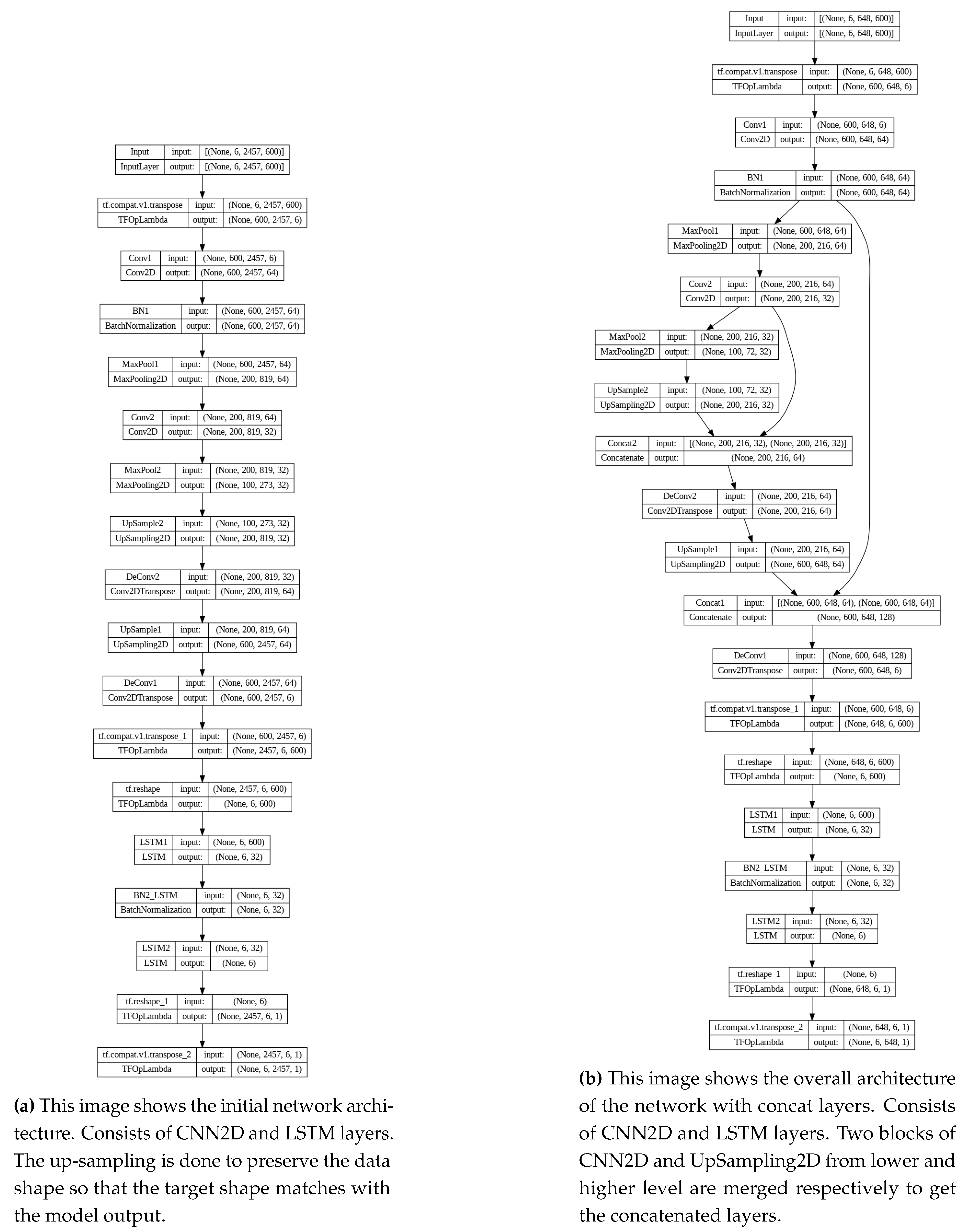
Next, we define a deep neural network consisting of convolutional layers to encode the spatial dependencies and then an LSTM layer to encode the long-term temporal dependencies. The model consists of 2 blocks of CNN-MaxPool layers followed by two blocks of Deconv-UpSample layers. After the convolution operation ends, the data is transposed so that the time dimension is the second axis for the temporal encoding to be efficiently encoded using LSTM. The tail of the network consists of 2 LSTM layers, with the first layer returning state values for each LSTM neuron while the last one only returns a single value Figure 1a illustrates this method.
Figure 1.
Model Architecture.
Figure 1.
Model Architecture.
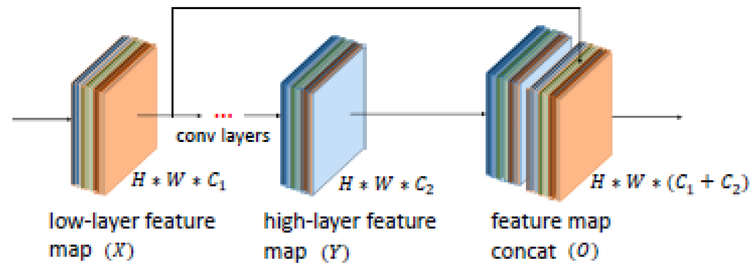
Figure 2.
Low-layer and high-layer features in CNN are combined directly.
Figure 2.
Low-layer and high-layer features in CNN are combined directly.
We also try to do some variations in the neural network architecture as well as on the dataset mentioned below:
The first variation consists of a model with 2D-CNN layers as initial layers, followed by hidden layers consisting of RNN layers and the last layer consists of Fully Connected Dense layers with an output layer with
k neurons, where
no. of counties The architecture is shown in Figure 3. The RNN layers are responsible for encoding the spatial lags. However, the data set is passed through a custom window slicer function to handle temporal lag. Early stopping is a method used to prevent a model from overfitting by ending the training process before it gets to the point of overfitting. Reducing the learning rate is used to make the optimization converge to the optimal solution more effectively during training. The performance matrix, namely the F1 score, was monitored during the training. These techniques get implemented when the data set’s performance metric does not improve for several epochs. Implementation of the early stopping stops the training and reduces the learning rate by a factor. The optimizer used to find a model/predictor
is Adam.
Adam is an optimization algorithm commonly used in machine learning to update the parameters of a model during training, using the first and second order moments [21]. The F1 loss is a performance metric used for evaluating the performance of current classification models, mainly when dealing with imbalanced datasets. It is derived from the F1 score, which is mathematically the harmonic mean of precision and recall.
Figure 3.
Model architecture of the first model variation. The input is fed to a 2D-CNN layer followed by RNN layer which is used for temporal encoding and finally is connected to a FC dense layer with sigmoid activations.
Figure 3.
Model architecture of the first model variation. The input is fed to a 2D-CNN layer followed by RNN layer which is used for temporal encoding and finally is connected to a FC dense layer with sigmoid activations.
- 2.
Certain municipalities in the dataset do not have a majority class. This means no information is available to the model from those specific instances. We filter out those municipalities, and we are left with 647 municipalities. Now, 647 is a prime number, and due to this reason, it will pose some difficulties in the max pooling and upsampling layers because max pooling reduces the dimension by half, and since 647 is not a multiple of two, three, or four, we will have to use either a valid padding, which again will have its own issues in making the output shape different from the target shape, or we can use a pooling window of size 647, which does not make any sense because a window size this large will fail to extract patterns from the feature maps. Hence, we randomly add a municipality from the discarded group of municipalities having only the majority class to make it 648. We can also argue that instead of adding, we could have removed a municipality, but this can only be known after we have experimented. We will refer to this dataset as the undersampled data in our literature.
- 3.
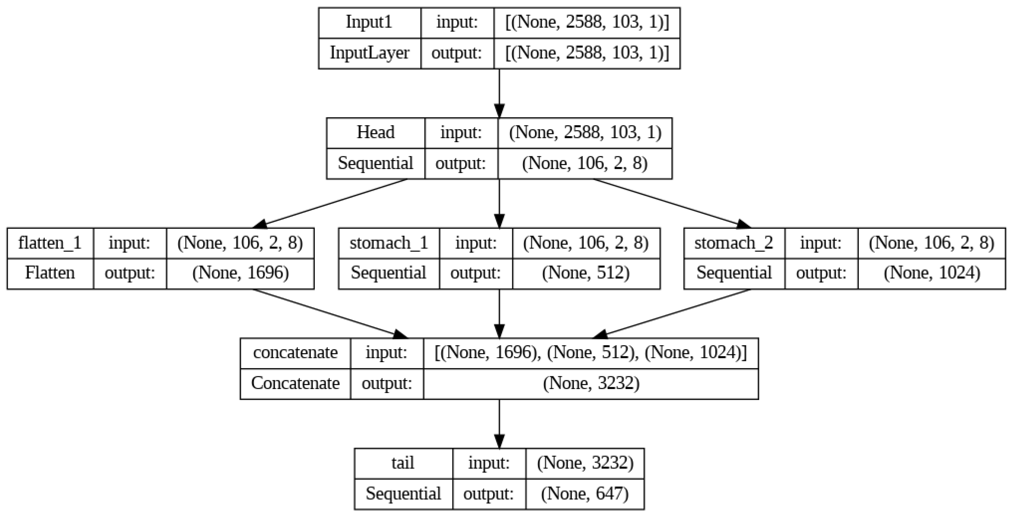
An improvement on the previous variation is built on top of the same pre-processed data with 647 counties, as mentioned in the first variation, are more complex than the previous one. Figure 4 shows that the output gets split into three branches after the input head. The first branch is a flatten layer, while the other two are structures of RNN. Then, all three of these get combined through the concatenate layer. Here, a skip connection is used to get more features for the next layer, ANN. The concatenated output goes to the ANN structure. The ANN structure is connected to the final output structure, with sigmoid activation at the output layer. This model’s training time is 3.15 minutes, 79.46 % less than the previous model.
Figure 4.
Architecture of model 2 with layers being split and concatenated at next stage for better results.
Figure 4.
Architecture of model 2 with layers being split and concatenated at next stage for better results.
- 4.
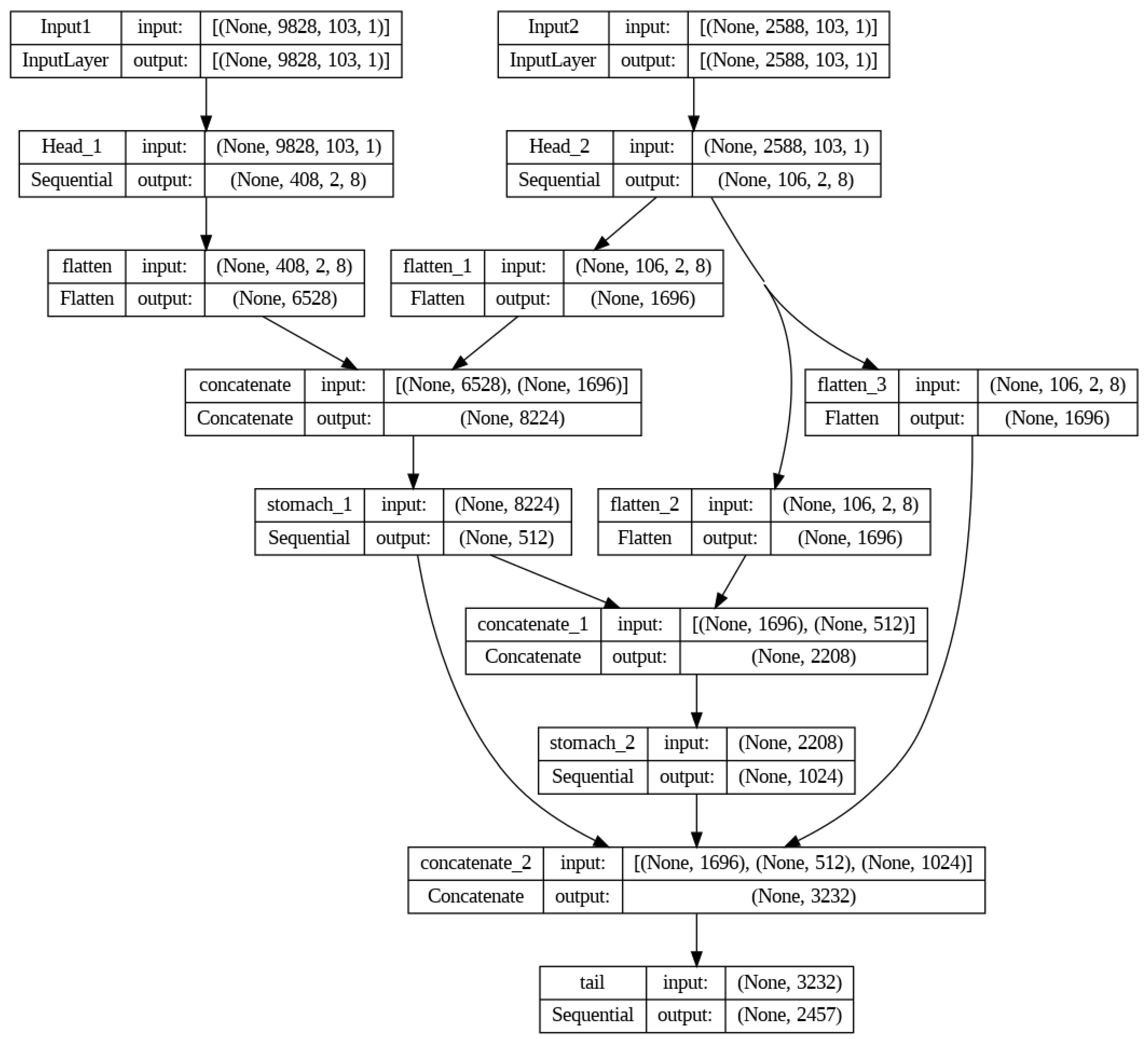
The third variation model has a two-headed input; the first head takes input X1, which has data for all 2457 counties and four months of lag. However, the second head takes input X2, which has data for only 647 counties mentioned in the previous model variation. The developed model is under the assumption that the head two will work as a way to oversample the minority Class 1 in this spatiotemporal data set. It is made with a similar structure of two-dimensional CNN layers as an initial part of the model; hidden layers contain RNN, and the model’s last part consists of ANN with an output layer of size 2457. The inputs are connected to Head 1 and Head 2, respectively. Heads are the CNN structures explicitly made for their inputs. Then, the data is passed down to Stomach 1 and Stomach 2 through the Flattening layer. The Stomach is composed of structures called RNNs that are specifically designed for processing its inputs. The final stage of the process involves passing the data to the tail block, which consists of ANN layers with a sigmoid activation function in the final layer. The Output from Head 1 and Head 2 are concatenated before passing through Stomach 1, while the Output of Stomach 1 and Head 2 is concatenated before passing through Stomach 2. Moreover, the Output of Stomach 1, Stomach 2, and Head 2 was concatenated before passing through the tail, as shown in Figure 5.
Figure 5.
Model 3 architecture with two headed input.
Figure 5.
Model 3 architecture with two headed input.
- 5.
It is a well-known and established fact that different layers in a CNN network can encode different levels of information. While low-level layers contain more detailed information than high-level ones, they suffer from background clutter and ambiguity. The high-level layers contain more semantic information than the low-level layers. State-of-the-art networks like U-Net combine multiple layers directly with much less training size and yield more precise segmentation. As shown in Figure 1b, in the combined feature map: , we use concatenation to merge two layers, one from the low-level and one from the high-level, both having the same spatial dimension except the one concatenated. Let layer L have a lower level feature map of dimension and layer R have a higher level feature map of dimension . Let the layer S denote the concatenation layer and the operator denote the concatenation operator which needs all the input dimensions to match except the concatenation axis. Then, denotes the concatenation operation with output feature map of shape .
- 6.
The final variation we use is by dissecting the data into two parts. The dataset is imbalanced as the majority class makes up 96 % of the proportion. In order to get around this, we propose a method. In-order to get around this, we propose a method. Let denote the actual dataset with the imbalance. Let denote the set of ratios of the counts of minority class w.r.t the majority class for all municipalities . Let denote the rank of the ratios . Let denote the data with top 6 municipalities with the count ratio such that and . denotes the position or the index of the value in the set. Let denote the remaining data such that . The distribution of majority and minority classes in will be much more stable or homogeneous compared to that of . This motivates us to train two different neural networks with the same concatenated layer but for two different datasets and independently. Because the first network has much less heterogeneity/imbalance compared to the second dataset, the first model will learn some important features that the previous one missed out, and the combination of these two models will also help reduce the bias-variance trade-off because the network trained on the first dataset will have much lesser bias compared to the previous version as the imbalance is reduced.
Finally, we train a weighted random forest on the original data as well as with the undersampled data where the weights are for each class . Hence, the class with less proportion will be weighted more so that the model assigns a relatively larger cost for misclassifying the minority class and a smaller cost for misclassifying the majority class. We use the custom F1-loss with Adam optimizer to compile the neural network model. Metrics used for this case are the F1 and ROC AUC scores because we have highly imbalanced data, with more than 96 % of labels belonging to the majority class. The learning rate of the optimizer is reduced by a factor of 0.2 if the validation AUC score does not improve for three consecutive epochs, training on 20 epochs with a validation split of 70:30.
3.1.3. Results
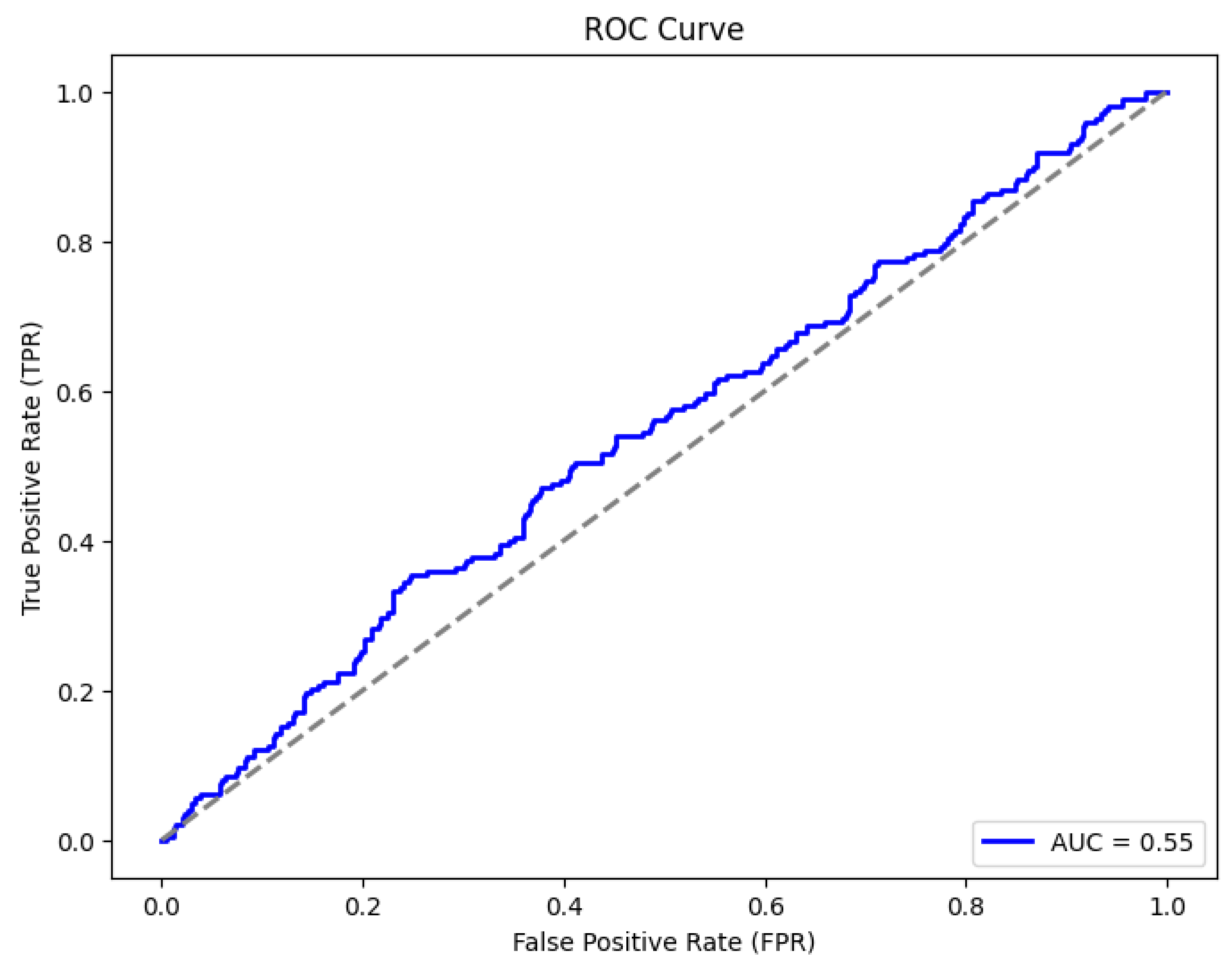
As presented in Table 1, the CNN2D+LSTM model trained on the original data performs poorly with an F1 score of just 1 % for the majority class on the test dataset and an AUC score of the majority class being 56 %. To our expectation, the random forest model performs significantly better with an F1 score of 15 % and an AUC score of the majority class of 76 %. Precision concerns about the accuracy of positive predictions. Hence, high precision indicates a low false positive rate, which is crucial when the cost of false positives is high. Recall, also termed sensitivity or true positive rate, assesses the accuracy of predicting positive instances among all actual positives. It emphasizes the capacity to identify positive instances accurately. High recall signifies a minimal false negative rate, crucial when overlooking positive instances that can yield severe consequences. The ROC-AUC score assesses the model’s effectiveness across diverse classification thresholds. It plots the TPR against the FPR thresholds and measures how well the model can segregate between the classes. A higher AUC score indicates a better discriminatory power of the model. The predict function returns a set of predicted probability scores for the majority class such that .
Table 1.
Test Set Evaluation on original dataset.
Table 1.
Test Set Evaluation on original dataset.
- 2.
We cannot just naively predict that
. The confidence/probability score we get from the model of the majority class
is upper bounded by 0.44, i.e.,
. Shown in
Table 2, for this case, we need to see how good is the model separability for each decile when the whole range of scores is divided into ten deciles. For this, we calculate the KS statistic using the decile method, i.e., by converting the predicted probability/scores into ten deciles and then measuring the separation between the cumulative distribution of the scores for each decile. Kolmogorov-Smirnov (KS) score measures the maximum difference between the cumulative distributions of positive and negative instances predicted by the model. It quantifies the model’s ability to separate the two classes, capturing the discriminatory power. A higher KS score indicates better classification performance. The decile with the largest separation is our decile of interest, and the separation between the cumulative distribution of positive and negative classes is the KS statistic. We use the lower endpoint of this decile as our threshold because, at this probability/confidence, the model can separate both classes best. To summarize, we use the condition
, where
denotes the lower endpoint of the decile having the largest separation.
Table 2.
KS table for CNN2D+LSTM network with original data. The value with green color shows the decile with the largest separation. The min_score column shows the lower endpoint of the decile while the max_score shows the higher endpoint of the decile. Here, bad_rate corresponds to and vice versa.
| Decile |
min_score |
max_score |
bad_rate |
good_rate |
cs_bads |
cs_goods |
sep |
| 1 |
0.387 |
0.441 |
0.47% |
99.53% |
20.60 |
9.98 |
10.62 |
| 2 |
0.381 |
0.387 |
0.21% |
99.79% |
29.90 |
19.98 |
9.92 |
| 3 |
0.371 |
0.381 |
0.23% |
99.77% |
40.20 |
29.88 |
10.22 |
| 4 |
0.366 |
0.371 |
0.20% |
99.80% |
49.17 |
39.98 |
9.19 |
| 5 |
0.356 |
0.366 |
0.08% |
99.92% |
52.82 |
49.99 |
2.83 |
| 6 |
0.330 |
0.356 |
0.35% |
99.65% |
68.11 |
59.98 |
8.12 |
| 7 |
0.327 |
0.330 |
0.20% |
99.80% |
76.74 |
69.98 |
6.76 |
| 8 |
0.325 |
0.327 |
0.14% |
99.86% |
83.06 |
79.99 |
3.06 |
| 9 |
0.312 |
0.325 |
0.11% |
99.89% |
88.04 |
90 |
1.96 |
| 10 |
0.286 |
0.312 |
0.27% |
99.73% |
100 |
100 |
0 |
- 3.
-
Table 4 shows the performance of the CNN2D+LSTM, with the same architecture as the previous network, and Balanced Random Forest on the undersampled data. The only change that happens while training the neural network is using F1-weighted loss instead of a vanilla custom F1 loss so that the misclassification of all classes is represented equally. The weighted F1 score is defined as , where represents the F1 score of the class k and represents the support or the number of actual occurrences of the class k in . Compared to the previous model, the F1 score on the test set has gone up to 25 % from 15 % for Random Forest, while the AUC score has reduced to 68 %, while there is only a slight increase for the CNN2D+LSTM model that goes to 2 % from 1 % and the AUC has slightly decreased to 52 %.
Table 3 shows the KS table for the CNN2D+LSTM model on the undersampled dataset for , where the lower endpoint of the decile having the largest separation is again used as the threshold for classifying into labels. From here on, every model is trained and evaluated on the undersampled dataset.
- 4.
-
Table 6 shows the performance of the data on the concatenated layers neural network architecture trained in the same fashion as above. The AUC score comes to 52 % with an F1 score of 2 %.
The KS table shown in Table 5 tells us that the decile with the maximum separation has decreased and dropped from the top 2 to the sixth decile.
- 5.
Similarly, Table 7 shows the performance of the two independent models trained on the dissected datasets and . The F1 score jumps to 5 % with an AUC score of 63 %. The KS score also improves to 24 %, and the decile range with the highest separation also increases to 69 % as seen in Table 8.
- 6.
Table 9 shows the performance of the neural network architecture’s first, third, and fourth variations. The F1 score, precision, and recall metrics are computed using three distinct confidence thresholds: 0.35, 0.50, and 0.65.
Table 3.
KS table for CNN2D+LSTM network with undersampled data. The value with green color shows the decile with the largest separation. The min_score column shows the lower endpoint of the decile while the max_score shows the higher endpoint of the decile. Here, bad_rate corresponds to and vice versa.
| Decile |
min_score |
max_score |
bad_rate |
good_rate |
cs_bads |
cs_goods |
sep |
| 1 |
0.473 |
0.539 |
0.86% |
99.14% |
9.97 |
10 |
0.04 |
| 2 |
0.459 |
0.473 |
1.29% |
98.71% |
24.92 |
19.96 |
4.96 |
| 3 |
0.452 |
0.459 |
0.74% |
99.26% |
33.55 |
29.97 |
3.58 |
| 4 |
0.446 |
0.452 |
0.74% |
99.26% |
42.19 |
39.98 |
2.21 |
| 5 |
0.437 |
0.446 |
0.91% |
99.09% |
52.82 |
49.98 |
2.85 |
| 6 |
0.428 |
0.437 |
0.77% |
99.23% |
61.79 |
59.98 |
1.81 |
| 7 |
0.404 |
0.428 |
1.11% |
98.89% |
74.75 |
69.96 |
4.79 |
| 8 |
0.397 |
0.404 |
0.77% |
99.23% |
83.72 |
79.97 |
3.75 |
| 9 |
0.364 |
0.397 |
0.91% |
99.09% |
94.35 |
89.96 |
4.39 |
| 10 |
0.297 |
0.364 |
0.49% |
99.51% |
100 |
100 |
0 |
Table 4.
Test Set Evaluation on undersampled dataset.
Table 4.
Test Set Evaluation on undersampled dataset.
Table 5.
KS table for CNN2D+LSTM network with concatenation layers. The value with green color shows the decile with the largest separation. The min_score column shows the lower endpoint of the decile while the max_score shows the higher endpoint of the decile. Here, bad_rate corresponds to and vice versa.
| Decile |
min_score |
max_score |
bad_rate |
good_rate |
cs_bads |
cs_goods |
sep |
| 1 |
0.534 |
0.567 |
0.74% |
99.26% |
8.64 |
10.01 |
1.38 |
| 2 |
0.525 |
0.534 |
1.14% |
98.86% |
21.93 |
19.99 |
1.94 |
| 3 |
0.507 |
0.525 |
0.57% |
99.43% |
28.57 |
30.01 |
10.44 |
| 4 |
0.479 |
0.507 |
0.97% |
99.03% |
39.87 |
40.00 |
0.13 |
| 5 |
0.469 |
0.3479 |
1.03% |
98.97% |
51.83 |
49.98 |
1.84 |
| 6 |
0.447 |
0.469 |
1% |
99% |
63.46 |
59.97 |
3.49 |
| 7 |
0.437 |
0.447 |
0.91% |
99.09% |
74.09 |
69.96 |
4.12 |
| 8 |
0.424 |
0.437 |
0.63% |
99.37% |
81.40 |
79.99 |
1.41 |
| 9 |
0.401 |
0.424 |
0.86% |
99.14% |
91.36 |
89.99 |
1.38 |
| 10 |
0.214 |
0.401 |
0.74% |
99.26% |
100 |
100 |
0 |
Table 6.
Test set evaluation of CNN2D+LSTM model with concatenation layers.
Table 6.
Test set evaluation of CNN2D+LSTM model with concatenation layers.
| Class |
Precision |
Recall |
F1 |
Support |
| 0 |
0.99 |
0.24 |
0.39 |
34691 |
| 1 |
0.01 |
0.78 |
0.02 |
301 |
Table 7.
Test set evaluation of CNN2D+LSTM model with two independent datsets along with concatenation layers.
Table 7.
Test set evaluation of CNN2D+LSTM model with two independent datsets along with concatenation layers.
| Class |
Precision |
Recall |
F1 |
Support |
| 0 |
0.99 |
0.90 |
0.94 |
34691 |
| 1 |
0.03 |
0.34 |
0.05 |
301 |
Table 8.
KS table for CNN2D+LSTM network with two independent datasets along with concatenation layers. The value with green color shows the decile with the largest separation. The min_score column shows the lower endpoint of the decile while the max_score shows the higher endpoint of the decile. Here, bad_rate corresponds to and vice versa.
| Decile |
min_score |
max_score |
bad_rate |
good_rate |
cs_bads |
cs_goods |
sep |
| 1 |
0.440 |
0.694 |
2.91% |
97.09% |
33.89 |
9.80 |
24.09 |
| 2 |
0.424 |
0.440 |
0.60% |
99.40% |
40.86 |
19.82 |
21.04 |
| 3 |
0.398 |
0.424 |
0.80% |
99.20% |
50.17 |
29.83 |
20.34 |
| 4 |
0.387 |
0.398 |
0.57% |
99.43% |
56.81 |
39.85 |
16.96 |
| 5 |
0.378 |
0.387 |
0.49% |
99.51% |
62.46 |
49.89 |
12.57 |
| 6 |
0.372 |
0.378 |
0.57% |
99.43% |
69.10 |
59.92 |
9.18 |
| 7 |
0.349 |
0.372 |
0.71% |
99.29% |
77.41 |
69.93 |
7.47 |
| 8 |
0.334 |
0.349 |
0.74% |
99.26% |
86.05 |
79.95 |
6.10 |
| 9 |
0.317 |
0.334 |
0.60% |
99.40% |
93.02 |
89.97 |
3.05 |
| 10 |
0.240 |
0.317 |
0.60% |
99.40% |
100 |
100 |
0 |
Table 9.
Evaluation Matrix.
Table 9.
Evaluation Matrix.
| Model |
Training |
Confidence |
Precision |
Recall |
F1 Score |
ROC |
KS |
| Name |
Time |
Level |
(Class 1) |
(Class 1) |
(Class 1) |
AUC |
Score |
| |
|
0.35 |
0.00 |
0.48 |
0.00 |
|
|
| NN_Model-1 |
15.34 min |
0.50 |
0.00 |
0.38 |
0.00 |
0.496 |
24.70 |
| |
|
0.65 |
0.01 |
0.33 |
0.02 |
|
|
| |
|
0.35 |
0.05 |
0.37 |
0.09 |
|
|
| NN_Model-2 |
3.15 min |
0.50 |
0.07 |
0.30 |
0.12 |
0.791 |
51.20 |
| |
|
0.65 |
0.15 |
0.20 |
0.15 |
|
|
| |
|
0.35 |
0.00 |
0.42 |
0.00 |
|
|
| NN_Model-3 |
10.43 min |
0.50 |
0.00 |
0.27 |
0.00 |
0.422 |
11.20 |
| |
|
0.65 |
0.01 |
0.20 |
0.02 |
|
|
3.2. Phase II
3.2.1. Motivation
The poor performance of the models with the selected variables motivates us to analyze the temporal signals of the data. As we used all the lags in our initial modeling, we want to analyze if those lags are even meaningful to start from in the first place. We perform a time series analysis of the dataset using all the six lagged files outlined in the sections below.
3.2.2. Analysis
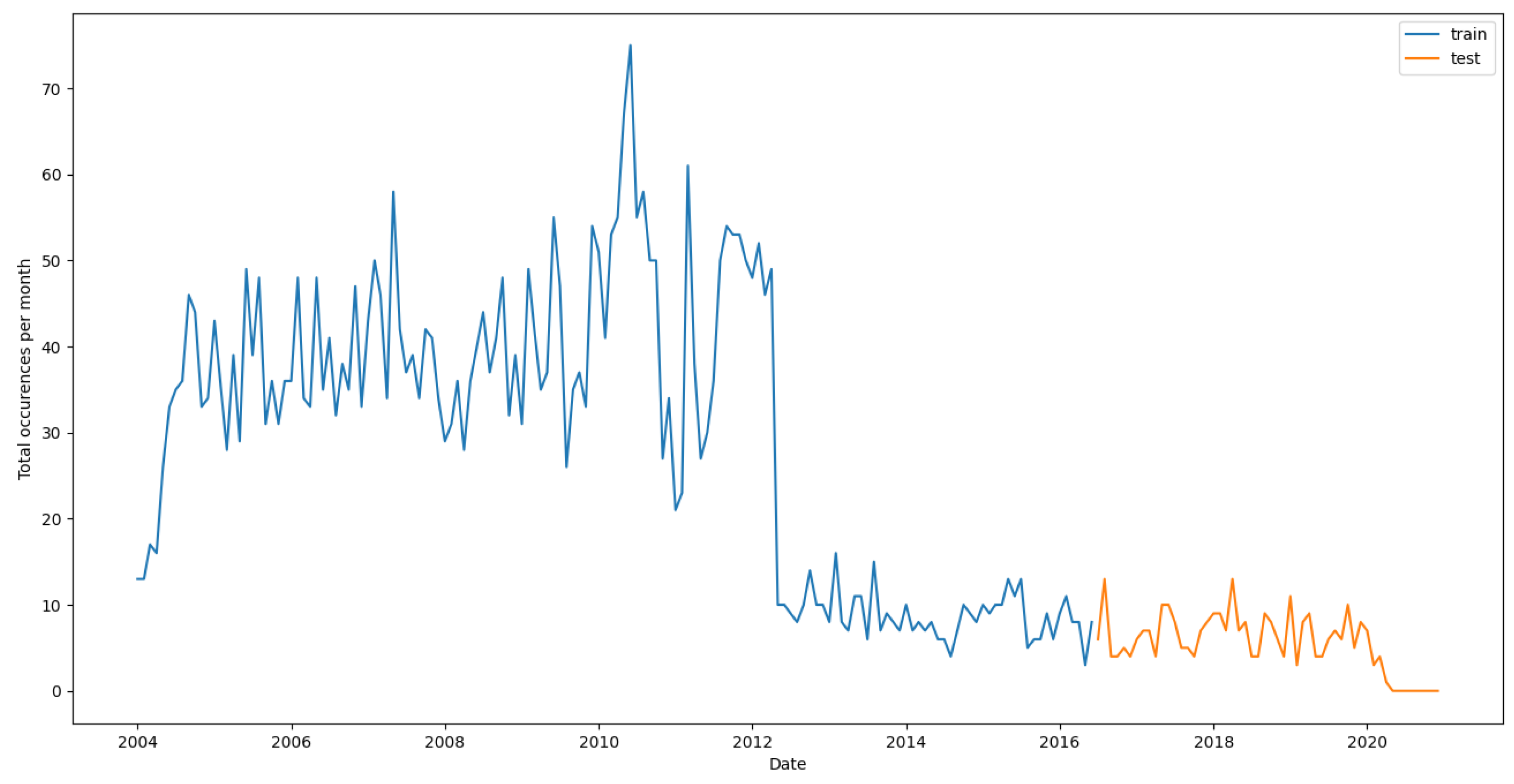
Following the conclusion, we use sampled monthly from 2004 to 2020 as the data points for analyzing the temporal signals without any exogenous variables from the features because we want to analyze how the counts of violent movements vary with time and its dependencies with past values .
Next, we split the data into training and testing, and the re-sampled monthly data of the counts is shown in Figure 6.
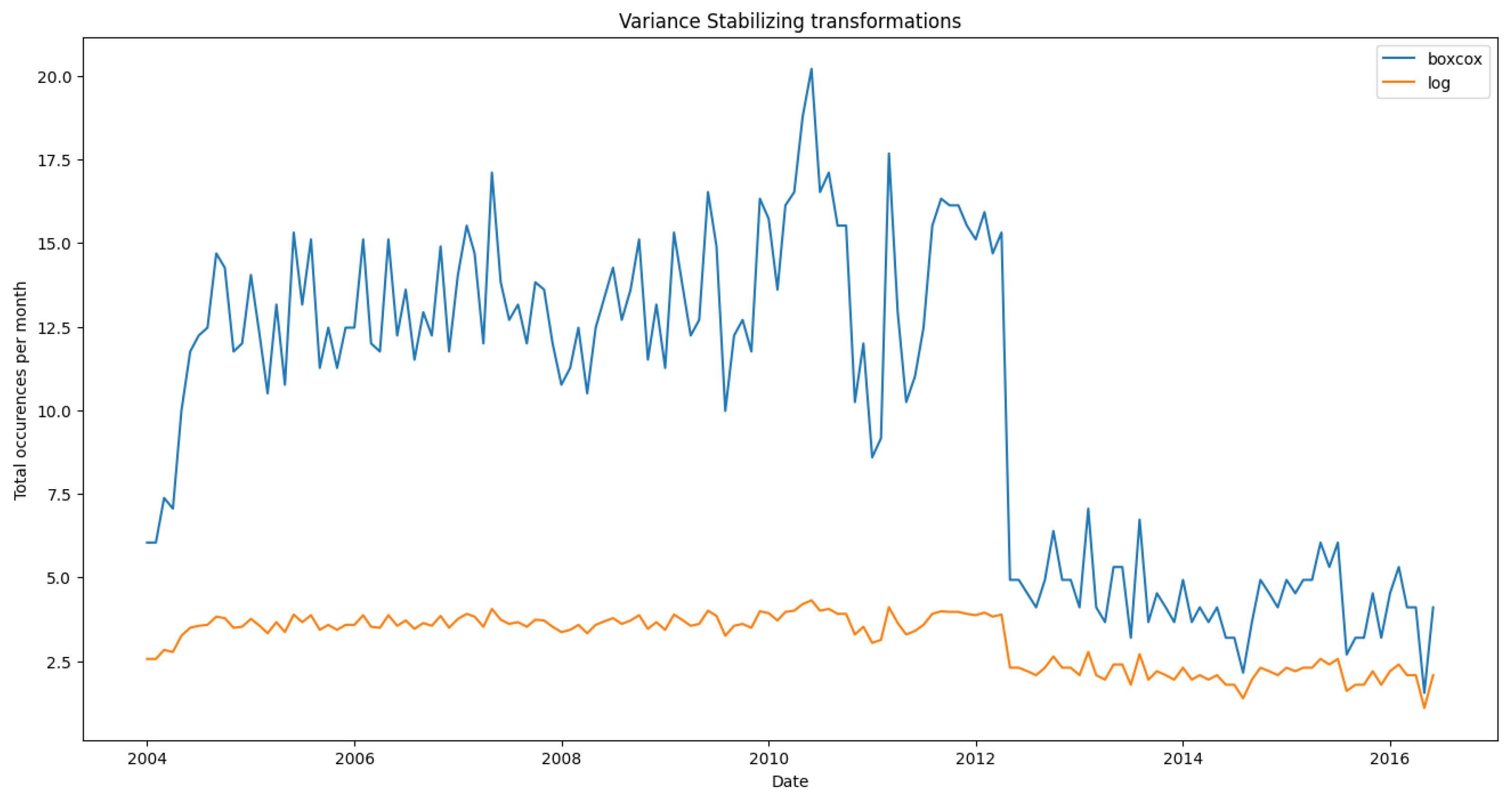
As it is evident, there is much variance in the data, so we will have to perform a variance stabilization transformation. We try both boxcox, given by as well as log transformation given by and the results of this transformation are shown in Figure 7.
Figure 6.
Monthly violence counts splitted into training and test.
Figure 6.
Monthly violence counts splitted into training and test.
Figure 7.
Comparison of the effects of Box-Cox and Log transformations on the original data to stabilize variance. Log transformation does a better job of stabilizing the variance.
Figure 7.
Comparison of the effects of Box-Cox and Log transformations on the original data to stabilize variance. Log transformation does a better job of stabilizing the variance.
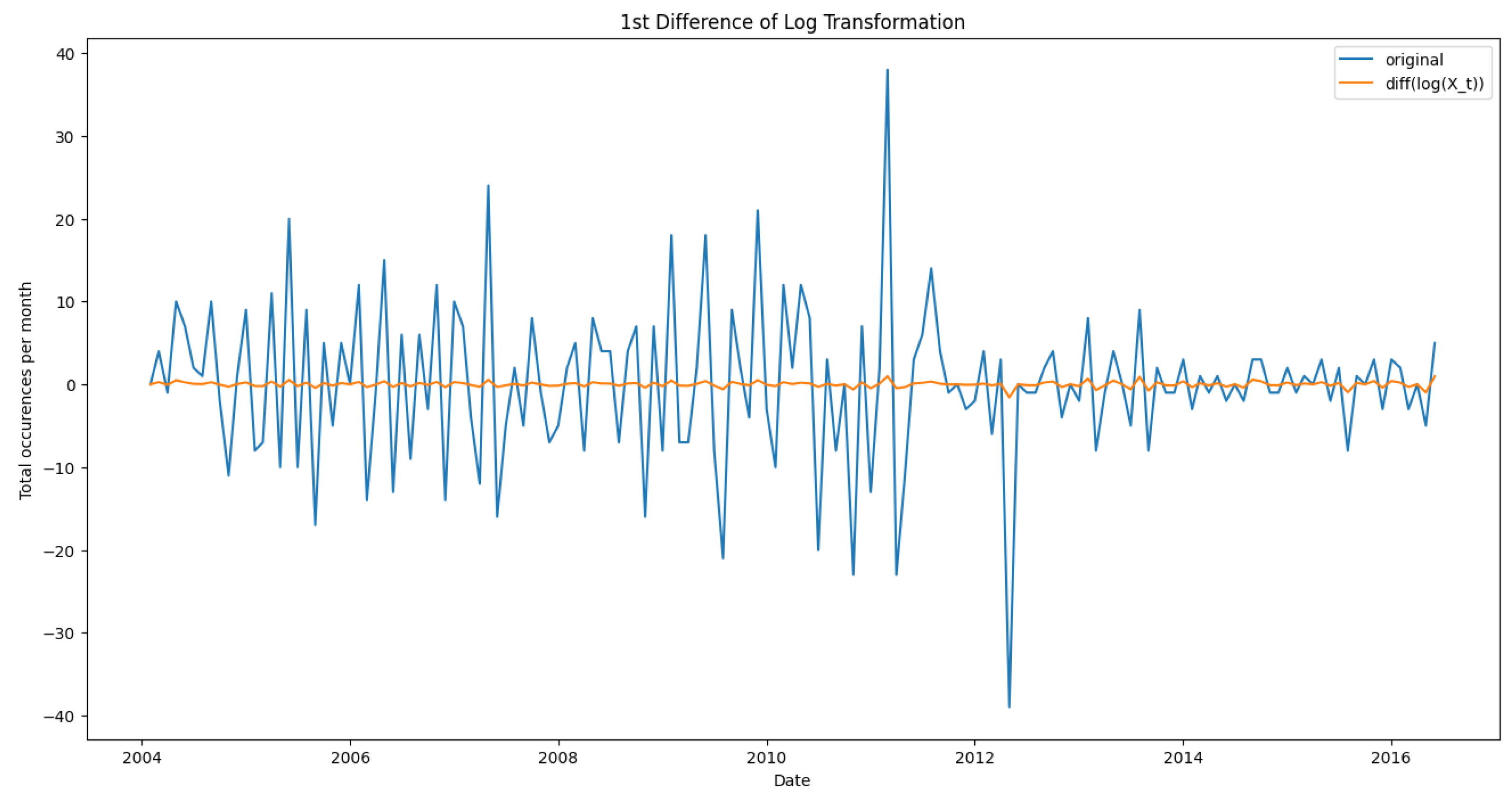
Now that the variance is stabilized, we must make the data stationary before fitting any model. For that, we take the first difference of the log-transformed series given by . Figure 8 shows the differenced variance transformed data compared to the differenced original data without any variance stabilization.
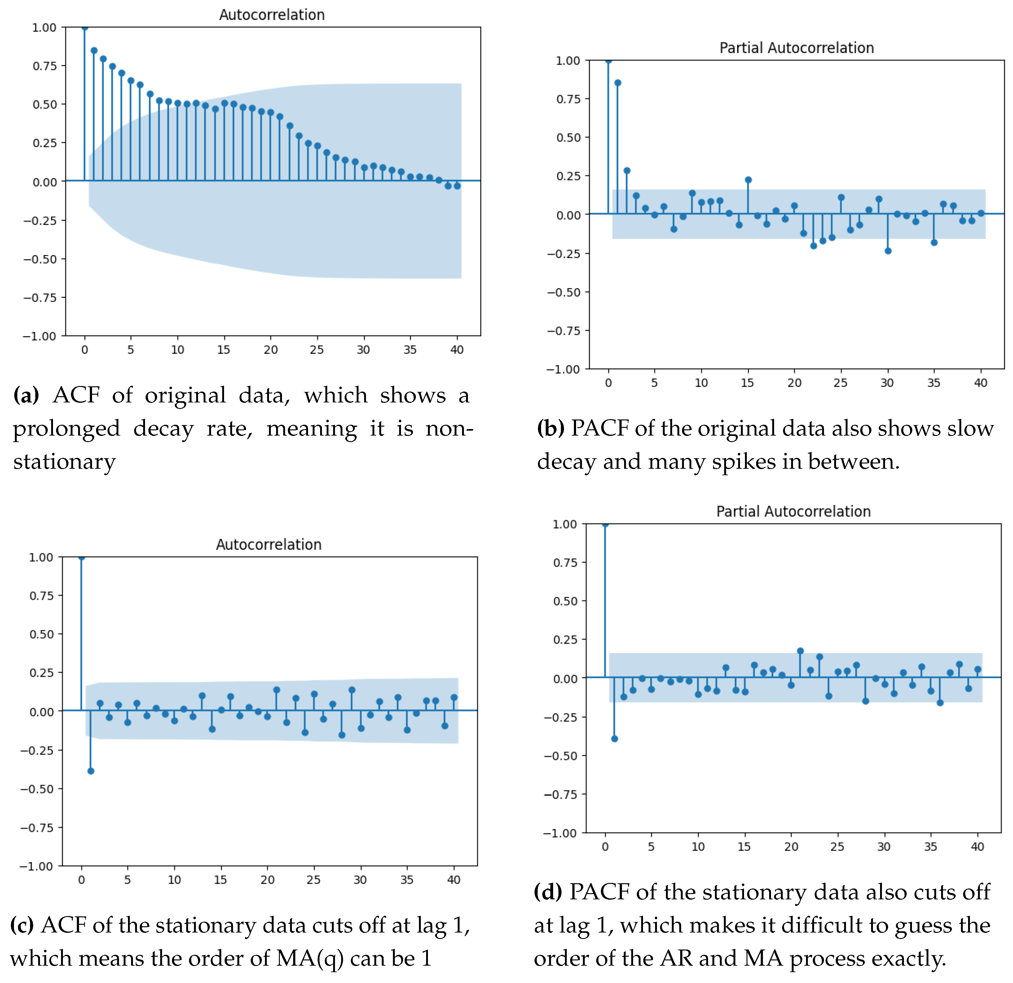
We can now fit an ARMA model to the data. but we need to figure out the parameters p and q for the AR, MA parts respectively, given by or can be written in compact form , where and represent the characteristic polynomial of the AR(p) and MA(q) process. We use the ACF and PACF plots to estimate the order of those characteristic polynomials to get the values of p and q. Figure 9 shows the ACF and PACF plot of the original data as well as the final transformed difference data. The ACF and PACF of the original data reveal the need for stationarity using differencing since the ACF is decaying very slowly. The ACF and PACF of the stationary data cut off at lag 1, which means we need to try a combination of models before we can estimate the right model parameters for the data.
Figure 8.
Comparison of differenced original data without variance stabilization versus differenced data with variance-stabilizing log transformation. The large wiggles on the original data show that stationarizing the data is insufficient. It also needs some variance stabilization due to the presence of noise.
Figure 9.
ACF and PACF plots for checking stationarity.
Figure 9.
ACF and PACF plots for checking stationarity.
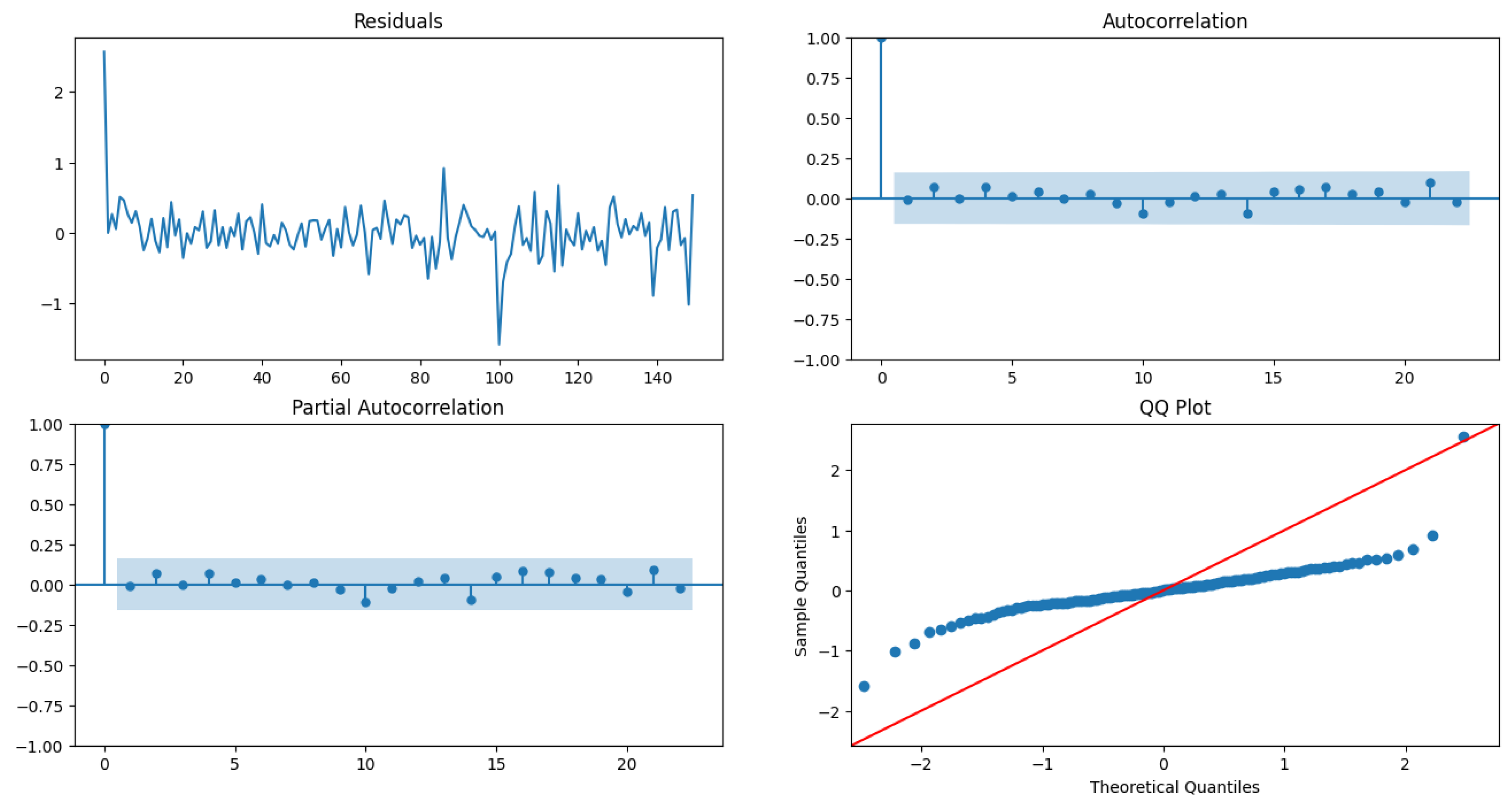
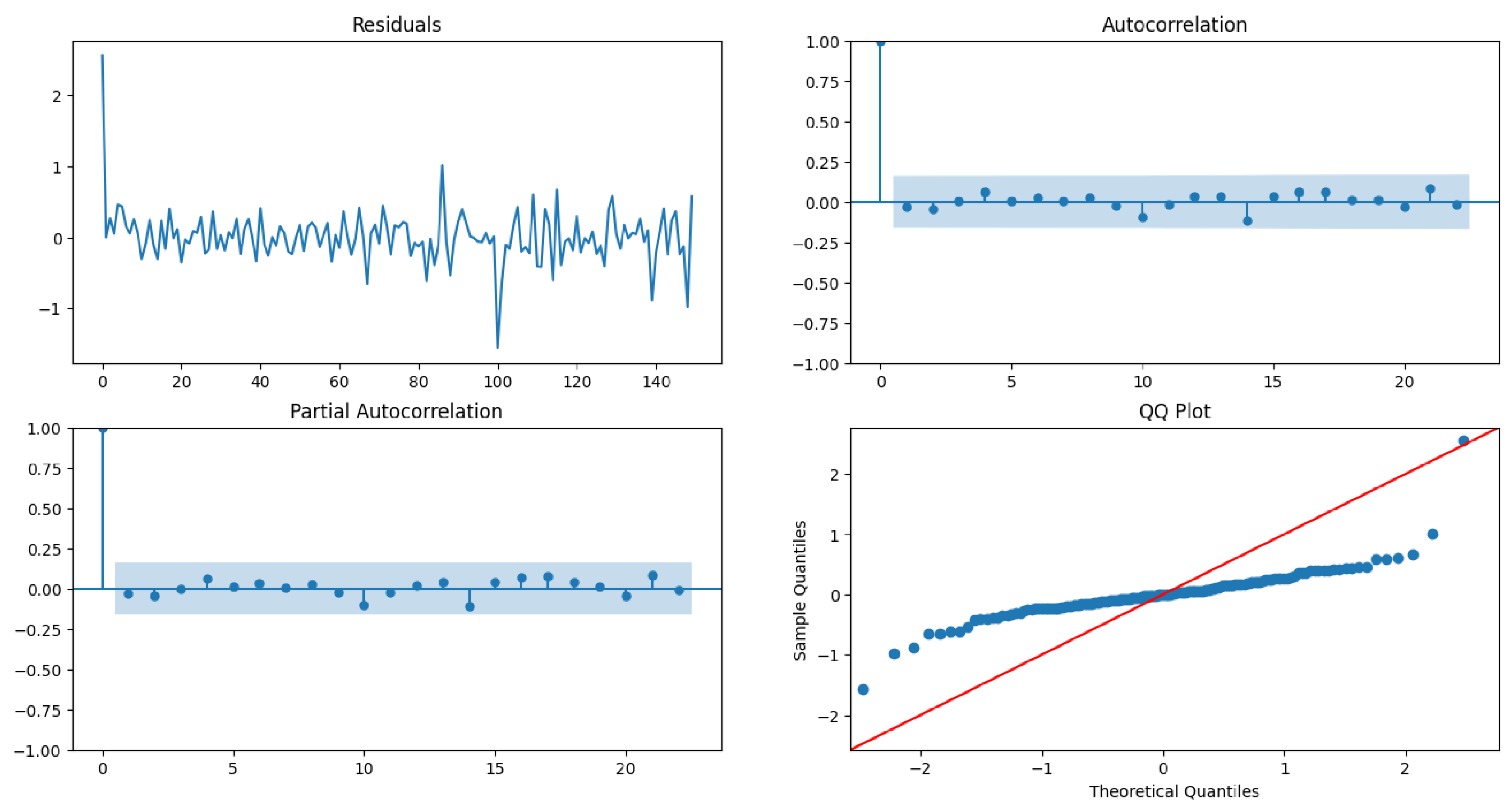
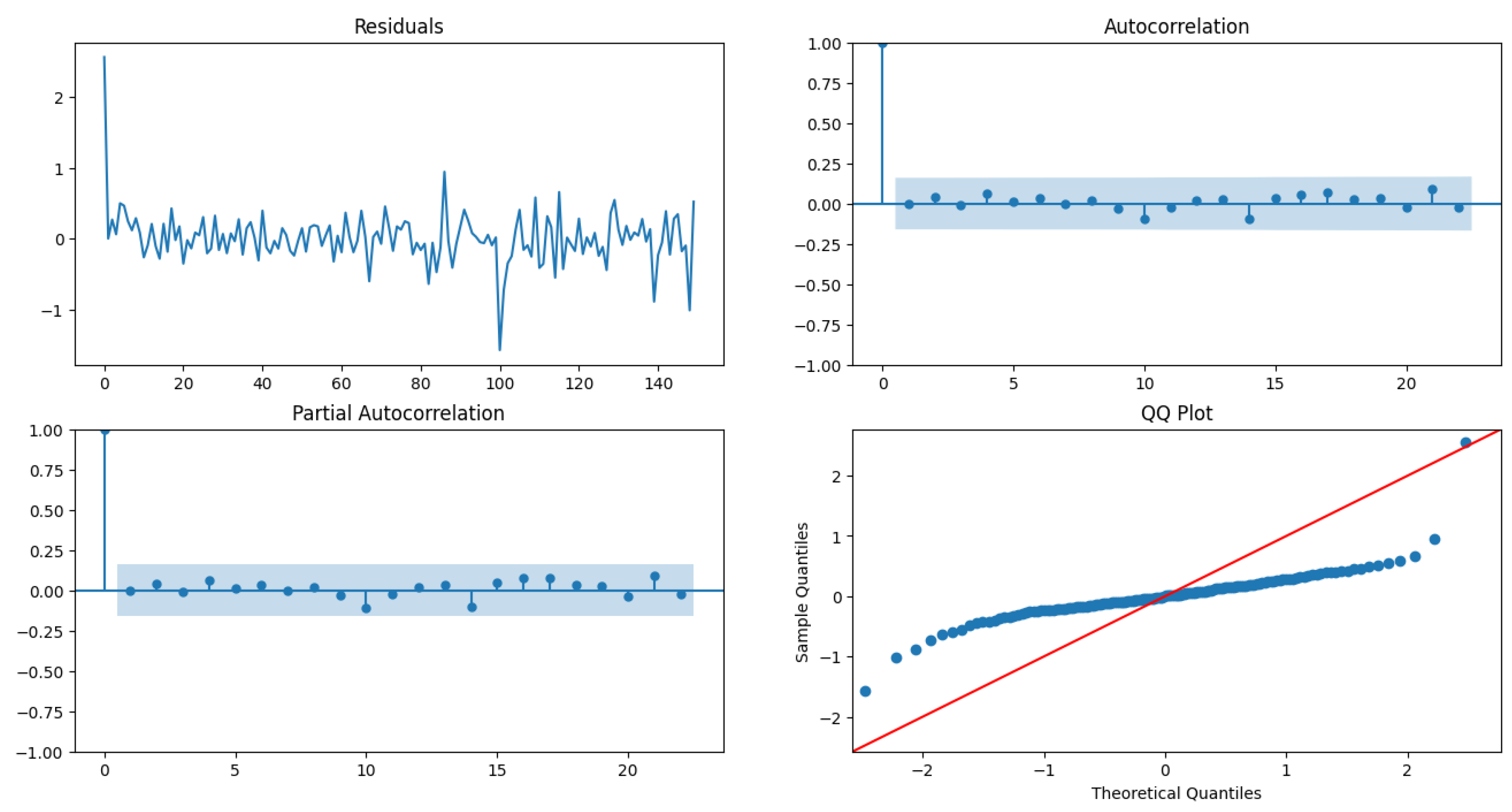
We fit three different models viz ARIMA(0,1,1), ARIMA(1,1,0), and ARIMA(1,1,1) on and measure the BIC of each model as well as perform residual diagnostics to select our best model. The model fit results are shown in Table 10, Table 11 and Table 12 whereas the residual plot diagnostics are shown in Figure 10, Figure 11 and Figure 12.
Figure 10.
Residual plot diagnostics for ARIMA(0,1,1).
Figure 10.
Residual plot diagnostics for ARIMA(0,1,1).
Figure 11.
Residual plot diagnostics for ARIMA(1,1,0).
Figure 11.
Residual plot diagnostics for ARIMA(1,1,0).
Figure 12.
Residual plot diagnostics for ARIMA(1,1,1).
Figure 12.
Residual plot diagnostics for ARIMA(1,1,1).
Table 10.
Model fit results of ARIMA(0,1,1) having a BIC of 90.
Table 10.
Model fit results of ARIMA(0,1,1) having a BIC of 90.
| Random Variable |
coef |
std err |
|
[0.025 |
0.975] |
| ma.L1 |
-0.4398 |
0.058 |
0.0 |
-0.554 |
-0.325 |
|
0.0987 |
0.006 |
0.0 |
0.086 |
0.111 |
Table 11.
Model fit results of ARIMA(1,1,0) having a BIC of 88.
Table 11.
Model fit results of ARIMA(1,1,0) having a BIC of 88.
| Random Variable |
coef |
std err |
|
[0.025 |
0.975] |
| ar.L1 |
-0.4082 |
0.064 |
0.0 |
-0.534 |
-0.282 |
|
0.1001 |
0.007 |
0.0 |
0.087 |
0.113 |
Table 12.
Model fit results of ARIMA(1,1,1) having a BIC of 92.
Table 12.
Model fit results of ARIMA(1,1,1) having a BIC of 92.
| Random Variable |
coef |
std err |
|
[0.025 |
0.975] |
| ar.L1 |
-0.1212 |
0.189 |
0.521 |
-0.491 |
0.249 |
| ma.L1 |
-0.3364 |
0.180 |
0.061 |
-0.689 |
0.016 |
|
0.0985 |
0.006 |
0.0 |
0.086 |
0.111 |
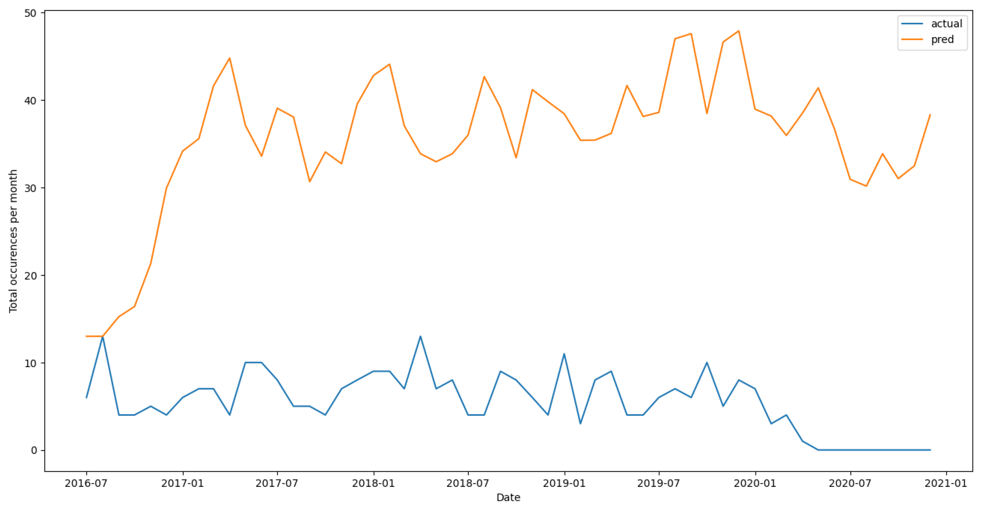
The model fit Table 10 shows evidence that ARIMA(1,1,0) has the least BIC, has a low model variance as well as low standard deviation for the estimate of the AR(1) coefficient , compared to other two models as shown in Table 11 and Table 12. The residuals plot diagnostics look pretty good, although the QQ plot of the residuals shows that they are not normally distributed and have a light tail. The ACF and PACF of the residuals do not have any random spikes, showing no auto-correlation between the residuals. The LB statistic has , which shows that the residuals are independent. The model is evaluated on the test data from 2016-07, as shown in Figure 13.
The Root Mean Squared Log Error on the test data is 2.07. The model can capture the data’s ups and downs but cannot learn the scale, as seen in the figure. All of these results point us to a conclusion: The model is a decent fit on the data but is very well spitting the fact that the univariate time series data of the counts of violent crimes is dependent on past 1 lag, i.e., . This motivates us to remove all the other lagged files and only use the first two files, and , outlined in the sections below.
Figure 13.
Model prediction results on unseen test data from 2016-07.
Figure 13.
Model prediction results on unseen test data from 2016-07.
3.2.3. Pre Processing
We first load the Lag 1 file into the memory. Then we filtered the data from 2004 because many demographical features like homicide and population were missing till 2003’s end. After filtering the data, we selected the 647 municipalities with majority and minority classes and discarded the rest. For this case, we do not add an extra municipality to make the count 648 because the CNN2D + LSTM architecture neural networks did not show much potential in the last phase, so we will not be training any of those architectures for this phase. Next, we select the top 300 features with the highest variance for this lagged file. The same procedure with the same features is used for the Lag2 file version to create 600 features. We then split the data at this stage into training and testing to prevent data leakage. Training data in until 2015-06, and the rest goes to test .
3.2.4. Methods
We first fit a couple of models that can handle the imbalanced data well with the default set of parameters to gauge the performance of the models on the new set of features. LightGBM classifier has the highest F1 score of 24 % followed by XGBoost with 23 % and random Forest with 23 %.
Hyperparameter tuning is a pivotal step in training the classifiers. It helps prevent overfitting by finding an optimal parameter space using various distributed methods like Grid Search CV and Randomized Search CV. We will primarily be restricting ourselves to Randomized Search CV because instead of trying out all possible given combinations like the Grid Search, it evaluates a given number of random combinations by selecting a random value for each hyperparameter at every iteration, and this approach has benefits like:
If we let the randomized search run for 1000 iterations, this approach will explore 1000 different values for each hyperparameter
Simply by setting the number of iterations, we have more control over the computing budget
Tuning gives optimal results for models like Random Forest and Decision Tree but gives suboptimal results for XGBoost and Light GBM. So, we stick to the default parameters for the latter models.
Once we have the tuned models, we fit a voting classifier using the three best-performing models viz decision tree, gradient boosting, and quadratic discriminant analysis classifier using both soft and hard voting. The former is defined as which predicts the class label as the class having the greater average of the predicted probabilities from each of the m models in the ensemble; while the latter is defined as which predicts the class label based on the majority vote from the m models.
Next, the voting classifier is evaluated on by trying three combinations of voting classifiers. The performance is measured using the F1 score, and the difference in precision and recall between the tied models breaks ties. Finally, the three different voting classifiers can be grouped into three different groups:
Voting Classifier 1: This voting classifier ensemble has a similar range of precision and recall scores, yielding the highest F1 score. This voting classifier uses a Decision Tree, Naive Bayes, QDA, and Light GBM.
Voting Classifier 2: These models have high precision but marginally low recall values, yielding a good F1 score. This voting classifier uses a Decision Tree, Light GBM, Random Forest, and XGBoost.
Voting Classifier 3: These models have low precision but significantly high recall values, again yielding a low F1 score. This voting classifier is formed using just QDA and Naive Bayes.
3.2.5. Results
Hyperparameter tuning using RandomisedSearchCV on the decision tree has led to a significant change in its F1 score and for Random Forest and XGBoost, while LightGBM’s F1 score after tuning stays the same. The QDA and Naive Bayes have poor precision but high recall, which means they predict most of them from minority classes and hence have large false positives.
As mentioned above, we have used voting classifiers with both soft as well as hard vote settings for different combinations of classifiers as follows:
Voting Classifier 1: This consists of Decision Tree(Tuned), QDA, Gaussian Naive Bayes and Light GBM(Baseline). The hard voting gave a significantly better result than the soft vote setting, which gives a high recall but very low precision.
Voting Classifier 2: This consists of Decision Tree(Tuned), Light GBM(Baseline), Random Forest(Tuned) and XGBoost(Baseline).
Voting Classifier 3: This consists of just QDA and Gaussian Naive Bayes and has a poor F1 score for both hard and soft settings because both are weak classifiers and produce an overall weak ensemble.
As we can see, using just the 600 features from the first two lagged files, we get a slightly better F1 score than the previous version of random forest, which acts as a benchmark for this version’s result. One thing to keep in mind for this section is that although we are trying to improve the performance of our model, we are more concerned with reducing the complexity of the model. The best-performing model was the voting classifier 1 with hard vote setting, an ensemble of Decision Trees (Tuned), Light GBM(Baseline), Random Forest(Tuned), and XGBoost(Baseline), which gave the highest F1 score of 26 % with a precision of 41 % and a recall of 18 %, better than all the standalone models. The hard methods do not have any AUC score since they cannot spit out a score because of the majority rule used as voting for the final class. The results can be seen in Table 13.
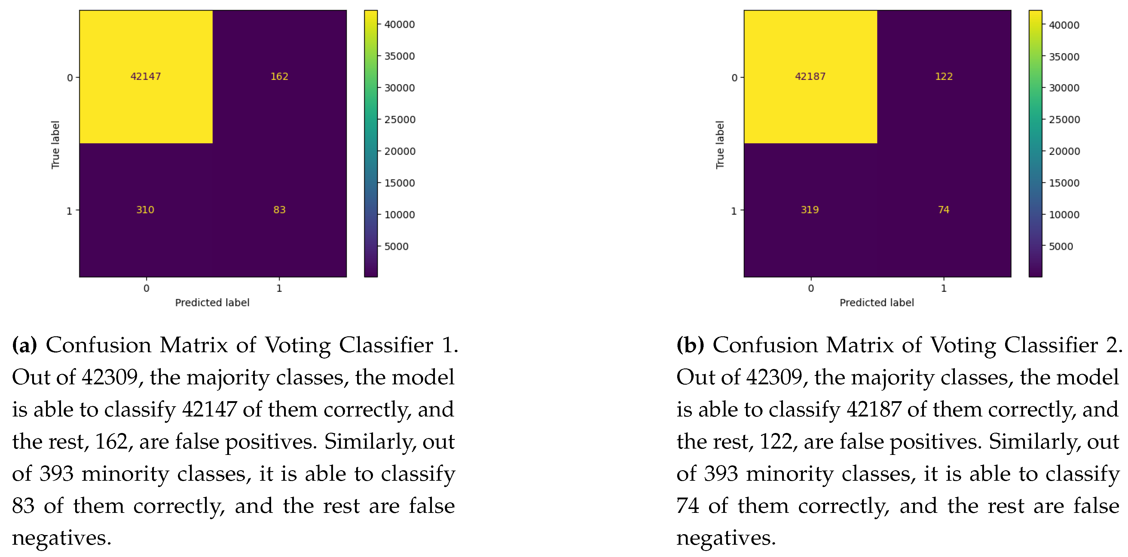
Figure 14 shows the performance of voting classifiers 1 and 2 on the test dataset. We can easily gauge the degree of imbalance in the dataset where the majority class distribution is almost 96 %. Considering this high imbalance, voting classifier 1 has high true negatives but low true positives compared to voting classifier 2. However, the difference is insignificant for the true positives, where the former has 83, and the latter has 74. On the contrary, voting classifier 1 has significantly fewer false positives than voting classifier 2, even though the latter performs marginally better than the former.
Table 13.
Evaluation on test set for the models tested on the new dataset from first 2 lagged files.
Table 13.
Evaluation on test set for the models tested on the new dataset from first 2 lagged files.
| Model |
Class |
Precision |
Recall |
F1 |
AUC |
Support |
| Decision tree(Baseline) |
0 |
0.99 |
0.94 |
0.97 |
0.42 |
442309 |
| Decision tree(Baseline) |
1 |
0.04 |
0.22 |
0.06 |
0.57 |
393 |
| Decision tree(Tuned) |
0 |
0.99 |
1 |
1 |
0.3 |
42309 |
| Decision tree(Tuned) |
1 |
0.68 |
0.14 |
0.23 |
0.69 |
393 |
| Random Forest(Baseline) |
0 |
0.99 |
1 |
1 |
0.3 |
42309 |
| Random Forest(Baseline) |
1 |
0.49 |
0.14 |
0.22 |
0.69 |
393 |
| Random Forest(Tuned) |
0 |
0.99 |
1 |
0.99 |
0.29 |
42309 |
| Random Forest(Tuned) |
1 |
0.36 |
0.19 |
0.25 |
0.7 |
393 |
| Gaussian Naive Bayes |
0 |
0.99 |
0.89 |
0.94 |
0.32 |
42309 |
| Gaussian Naive Bayes |
1 |
0.04 |
0.45 |
0.07 |
0.69 |
393 |
| LightGBM(Baseline) |
0 |
0.99 |
0.99 |
0.99 |
0.3 |
42309 |
| LightGBM(Baseline) |
1 |
0.25 |
0.24 |
0.24 |
0.69 |
393 |
| LightGBM(Tuned) |
0 |
0.99 |
0.99 |
0.99 |
0.29 |
42309 |
| LightGBM(Tuned) |
1 |
0.28 |
0.22 |
0.24 |
0.70 |
393 |
| XGBoost(Baseline) |
0 |
0.99 |
0.99 |
0.99 |
0.33 |
42309 |
| XGBoost(Baseline) |
1 |
0.25 |
0.22 |
0.23 |
0.66 |
393 |
| XGBoost(Tuned) |
0 |
0.99 |
0.99 |
0.99 |
0.30 |
42309 |
| XGBoost(Tuned) |
1 |
0.28 |
0.23 |
0.25 |
0.69 |
393 |
| QDA |
0 |
0.99 |
0.83 |
0.99 |
0.31 |
42309 |
| QDA |
1 |
0.03 |
0.52 |
0.05 |
0.69 |
393 |
| Voting Classifier 1(Hard) |
0 |
0.99 |
1 |
0.99 |
NA |
42309 |
| Voting Classifier 1(Hard) |
1 |
0.34 |
0.21 |
0.26 |
NA |
393 |
| Voting Classifier 1(Soft) |
0 |
0.99 |
0.89 |
0.94 |
0.29 |
42309 |
| Voting Classifier 1(Soft) |
1 |
0.04 |
0.45 |
0.07 |
0.70 |
393 |
| Voting Classifier 2(Hard) |
0 |
0.99 |
1 |
0.99 |
NA |
42309 |
| Voting Classifier 2(Hard) |
1 |
0.38 |
0.19 |
0.25 |
NA |
393 |
| Voting Classifier 2(Soft) |
0 |
0.99 |
1 |
0.99 |
0.29 |
42309 |
| Voting Classifier 2(Soft) |
1 |
0.3 |
0.2 |
0.24 |
0.7 |
393 |
| Voting Classifier 3(Hard) |
0 |
0.99 |
0.89 |
0.94 |
NA |
42309 |
| Voting Classifier 3(Hard) |
1 |
0.04 |
0.45 |
0.07 |
NA |
393 |
| Voting Classifier 3(Soft) |
0 |
0.99 |
0.89 |
0.94 |
0.31 |
42309 |
| Voting Classifier 3(Soft) |
1 |
0.04 |
0.45 |
0.07 |
0.7 |
393 |
Figure 14.
Confusion Matrix of Voting Classifier 1 and 2 on test data.
Figure 14.
Confusion Matrix of Voting Classifier 1 and 2 on test data.
The fact that we can get the same performance with fewer features tells us that this model is much more parsimonious and, hence, less complex according to Occam’s razor, hence achieving what our main goal for this section was. This further motivates us to perform full-scale feature selection using the state-of-the-art efficient variable selection methods widely present in the literature.
3.3. Phase III
3.3.1. Motivation
There was a significant improvement in the classical machine learning models compared to the initial modeling with all the lagged files. However, we saw that the time series model could not generalize the data well, so the actual and predicted were slightly off in scale. Examining the QQ plot shows us an apparent deviation from normality, with a light-tailed skewness. This means there are some missing terms in the model fit.
As described in the previous section, the best-performing voting classifier is trained on a large feature space of 600 predictors with just two lag files, which makes the model very complex and less parsimonious for unseen new data and hence is less generalized and more prone to overfitting.
These analyses give us an undeniable conclusion: apart from just two lags, there might be a combination of features from the exhaustive list of predictors, which might be smaller and give better results. The third modeling phase focuses on feature selection from all the lagged files.
3.3.2. Pre Processing
Similar to the last section, we first load all the six lagged files in the memory, selecting all the 1210 predictors from each file, which makes the final dataset with 518247 samples and 7260 predictors. Next, we filtered the data from 2004 and removed records with municipalities that did not have the minority class. For this section, we add one extra municipality to make the total municipalities count as 648, as we would also experiment with the neural network architecture. In this case, we split the data in a 70:30 split for all the classical algorithms because we are not considering the spatiotemporal structure when using the classical methods, while the split for the spatiotemporal structure for neural network experiments stays the same.
3.3.3. Methods
As outlined in the above sections, we use various variable selection methodologies to select important variables to get a lower dimensional feature space, thus making the model more parsimonious. We use a two-stage approach to identify a good subset of predictors and a good performing model, using the Voting Classifier 1 with hard voting as the baseline by tuning the model on the validation set. First, we use a base classifier(Random Forest in our case) to get hold of the subset of feature space. Secondly, we then tune various models to optimize the predictive performance of the models on the selected feature space. We start with the three most common methods as outlined below:
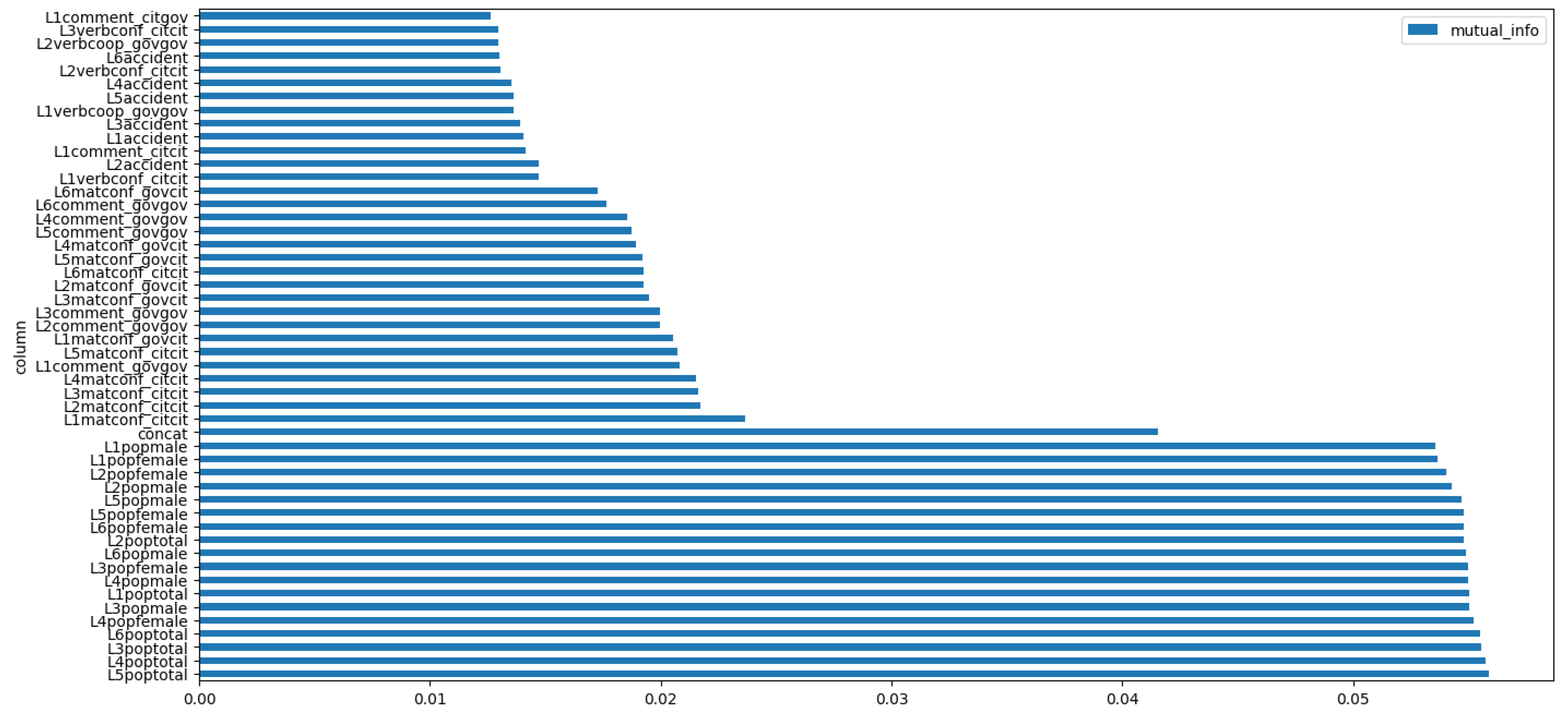
Mutual Information Gain: Mutual Information is a non-negative measure indicating the dependency between two random variables. It equals zero only when the variables are independent, and larger values indicate stronger dependency. The technique utilizes nonparametric approaches derived from entropy estimation using distances from k-nearest neighbors as described in [22] and [34]. Let be a pair of random variables, where X acts as a predictor and Y acts as a target, where the values are over the space . If their joint distribution is and the marginal distributions are and , the mutual information is defined as , where is the Kullback-Leibler divergence.
Forward Stepwise Regression: Stepwise regression is a technique for constructing regression models wherein the selection of predictive variables is automated. At each step, a variable from the set of predictors is evaluated for inclusion based on a predefined threshold, typically the p-value of the resultant variable upon addition to the model. Since our task is a classification problem, we first fit a logistic regression model with just a constant and no predictors. Then, we iterate over all the predictors and select the predictor whose addition results in the most significant p-value of the added predictor. Similarly, the process goes on until there is no significant improvement in p-value after adding any variable. One thing to note is that since this method adds new predictors in a stepwise fashion instead of a greedy fashion, it will only give suboptimal results.
Recursive Feature Elimination (RFE) is a wrapper-style feature selection algorithm [15]. It utilizes a different classifier within its core and is wrapped by RFE to aid in feature selection. This differs from filter-based feature selection methods that assess each feature individually and select those with the highest scores. RFE combines wrapper-style and filter-based feature selection techniques by internally using filter-based methods. It accomplishes this by fitting the specified classifier, ranking predictors by importance, discarding the least important features iteratively, and refitting the model. This process continues until a predetermined number of features remain. Each predictor receives a range of ranks, with the selected features assigned a rank of 1.
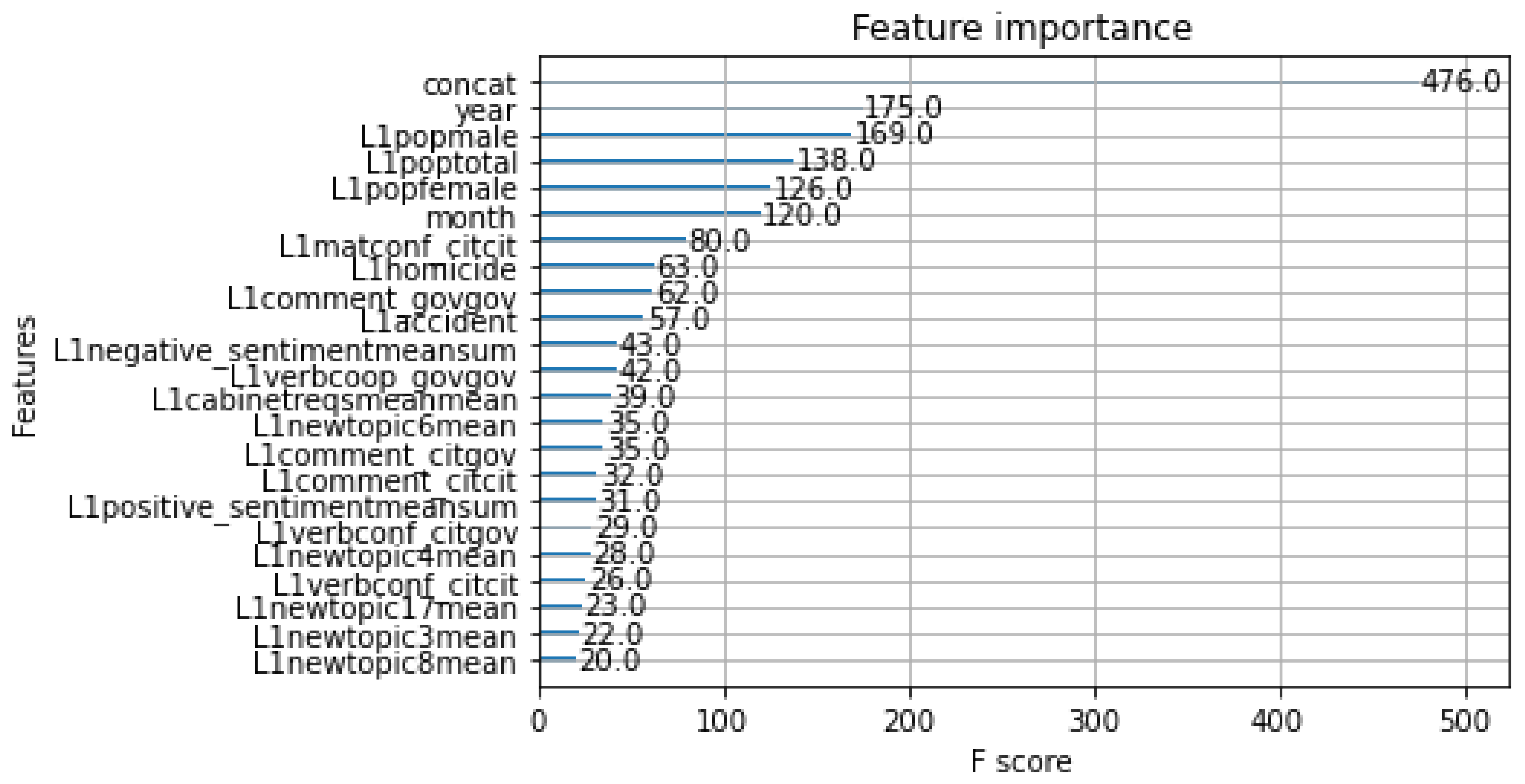
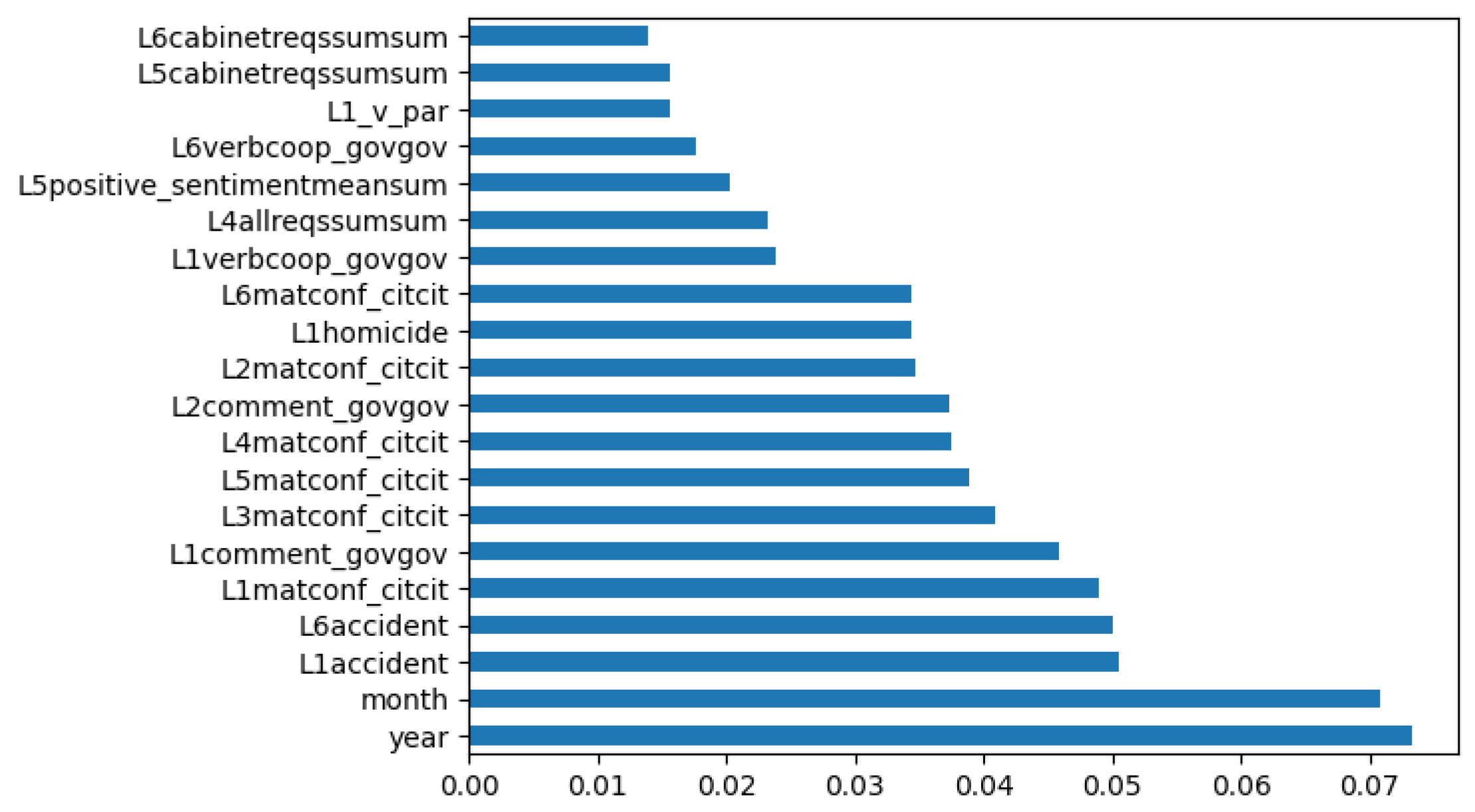
Feature Importance: We utilize a robust algorithm called XGBoost [6] to train a model on our dataset. This algorithm leverages multiple decision trees to make highly accurate predictions. During the training process, the model is fed with various features and their corresponding target variables. Once the model is trained, it generates a feature importance score for each feature in the dataset. This score is derived using the gain metric, which measures the improvement in the model’s objective function when a particular feature is split. A higher gain value indicates that the feature is more important than others. We then rank the features based on their importance scores to identify the most influential ones in the dataset. Features with higher importance scores are more informative in predicting the target variable. This approach helps us to understand which features are most relevant to our prediction task, enabling us to make more informed decisions. The Figure 15 shows that features, namely L1poptotal, L1popmale, L1matconf_citcit, L1homicide, L1accident, and month are critical features selected by the model when trained using the data pre-processed from sliding window approach.
Figure 15.
Relative Feature Importance from Random Forest using sliding window approach.
Figure 15.
Relative Feature Importance from Random Forest using sliding window approach.
- 5.
Principal Component Analysis (PCA): Principal Component Analysis (PCA) [18,32,42] is a statistical method designed to condense high-dimensional data into a lower-dimensional space while preserving essential information. It reduces dimensionality by identifying a new set of orthogonal variables known as principal components. These components represent linear combinations of the original variables and are ordered according to the variance they capture in the data. The first principal component captures the most significant variance, with subsequent components capturing the maximum remaining variance orthogonal to the preceding ones. PCA is valuable for exploring and visualizing complex data structures and patterns, particularly in high-dimensional datasets. By reducing dimensionality, PCA helps mitigate challenges such as the curse of dimensionality, which arises from the increased complexity and sparsity of data as dimensions increase. Additionally, PCA aids in feature extraction and data compression, as the lower-dimensional representation requires less storage and computational resources. This approach proves advantageous, mainly when applied with Support Vector Machines, particularly when handling extensive datasets like those from Mexico.
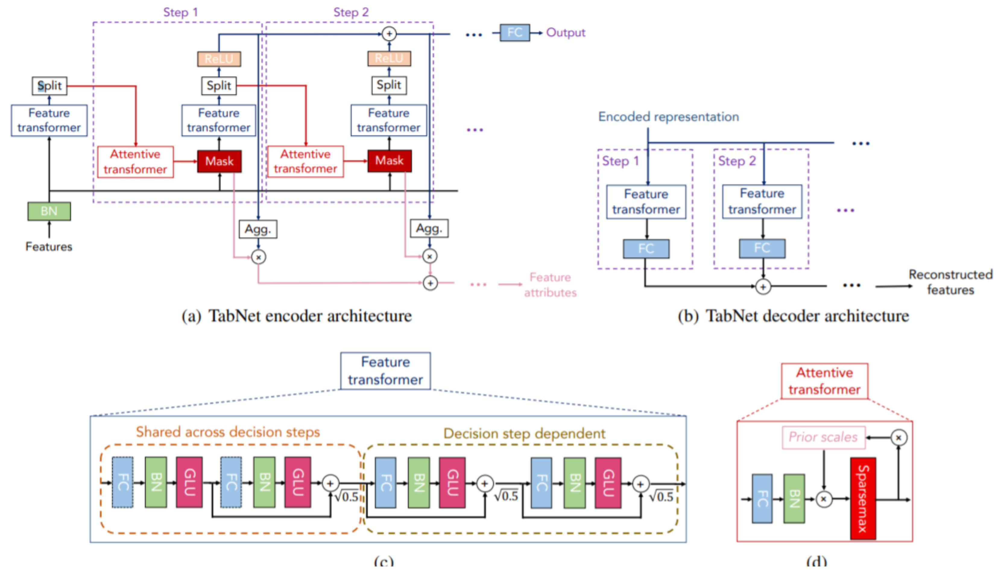
To train the data, we fit several classical machine learning models like XGBoost, CatBoost, LightGBM, and SVM. We also use the state-of-the-art TabNet neural network, designed explicitly for tabular datasets. TabNet [4] is a deep learning model designed for tabular data, capturing complex relationships and making accurate predictions. TabNet uses a method that combines a structured attention mechanism and a sequential decision-making process to find and use valuable features. The model architecture consists of multiple decision steps comprising an encoder and an attentive transformer. TabNet identifies significant features and runs them through the encoder during each decision step. The encoder then applies a sequence of transformations, resulting in feature representations. The feature selection process in TabNet is governed by a binary gating mechanism, enabling the model to focus on relevant features while suppressing noise. After the encoder output, the attentive transformer takes over and conducts another round of transformations to create high-level representations. The final prediction is made using a prediction head that takes the output from the attentive transformer and produces the desired output. As mentioned earlier, we use the sliding window concept on the first lag file to generate lagged features, which are used to train and evaluate the models.
Figure 16.
Structure of TabNet.
Figure 16.
Structure of TabNet.
Ensemble models combine the predictions of multiple individual models to create a more robust and accurate final prediction. The ensemble of XGBoost, LightGBM, CatBoost, and TabNet leverages the unique strengths of each model to improve predictive performance. XGBoost, LightGBM, CatBoost, and TabNet are machine-learning algorithms with outstanding performance in different tasks and domains. They are powerful tools to consider. Each model has its distinct characteristics and advantages. By combining these models, we can leverage their diverse approaches, enabling us to capture different patterns and information within the data. This ensemble approach helps mitigate the limitations and biases of individual models, leading to enhanced predictive power—the ensemble constructed here by combining the individual predictions using a weighted average. The ensemble model benefits from the collective intelligence of these state-of-the-art algorithms. XGBoost, LightGBM, CatBoost, and TabNet excel in different aspects, such as handling gradient boosting, categorical features, and attention-based modeling. The combination allows us to leverage their strengths and improve overall predictive accuracy. Table 14 shows the performance of the models.
Table 14.
Evalution Matrix.
Table 14.
Evalution Matrix.
| Model |
Training |
Confidence |
Precision |
Recall |
F1 Score |
ROC |
KS |
| Name |
Time |
Level |
(Class 1) |
(Class 1) |
(Class 1) |
AUC |
Score |
| |
|
0.35 |
0.35 |
0.19 |
0.25 |
|
|
| XGBoost |
1.85 min |
0.50 |
0.50 |
0.15 |
0.23 |
0.855 |
53.00 |
| |
|
0.65 |
0.56 |
0.11 |
0.19 |
|
|
| |
|
0.35 |
0.06 |
0.08 |
0.07 |
|
|
| LightGBM |
0.15 min |
0.50 |
0.09 |
0.06 |
0.07 |
0.828 |
48.60 |
| |
|
0.65 |
0.15 |
0.06 |
0.09 |
|
|
| |
|
0.35 |
0.35 |
0.19 |
0.24 |
|
|
| CatBoost |
3.8 min |
0.50 |
0.44 |
0.17 |
0.25 |
0.843 |
48.19 |
| |
|
0.65 |
0.53 |
0.16 |
0.24 |
|
|
| |
|
0.35 |
0.34 |
0.12 |
0.17 |
|
|
| TabNet |
51.36 min |
0.50 |
0.57 |
0.08 |
0.15 |
0.822 |
48.10 |
| |
|
0.65 |
0.00 |
0.00 |
0.00 |
|
|
| |
|
0.35 |
0.39 |
0.16 |
0.23 |
|
|
| Ensemble |
57.16 min |
0.50 |
0.59 |
0.11 |
0.19 |
0.847 |
50.10 |
| |
|
0.65 |
0.70 |
0.05 |
0.12 |
|
|
| |
|
0.35 |
0.40 |
0.08 |
0.13 |
|
|
| SVM |
31.6 min |
0.50 |
0.42 |
0.07 |
0.13 |
0.574 |
2.19 |
| |
|
0.65 |
0.40 |
0.06 |
0.10 |
|
|
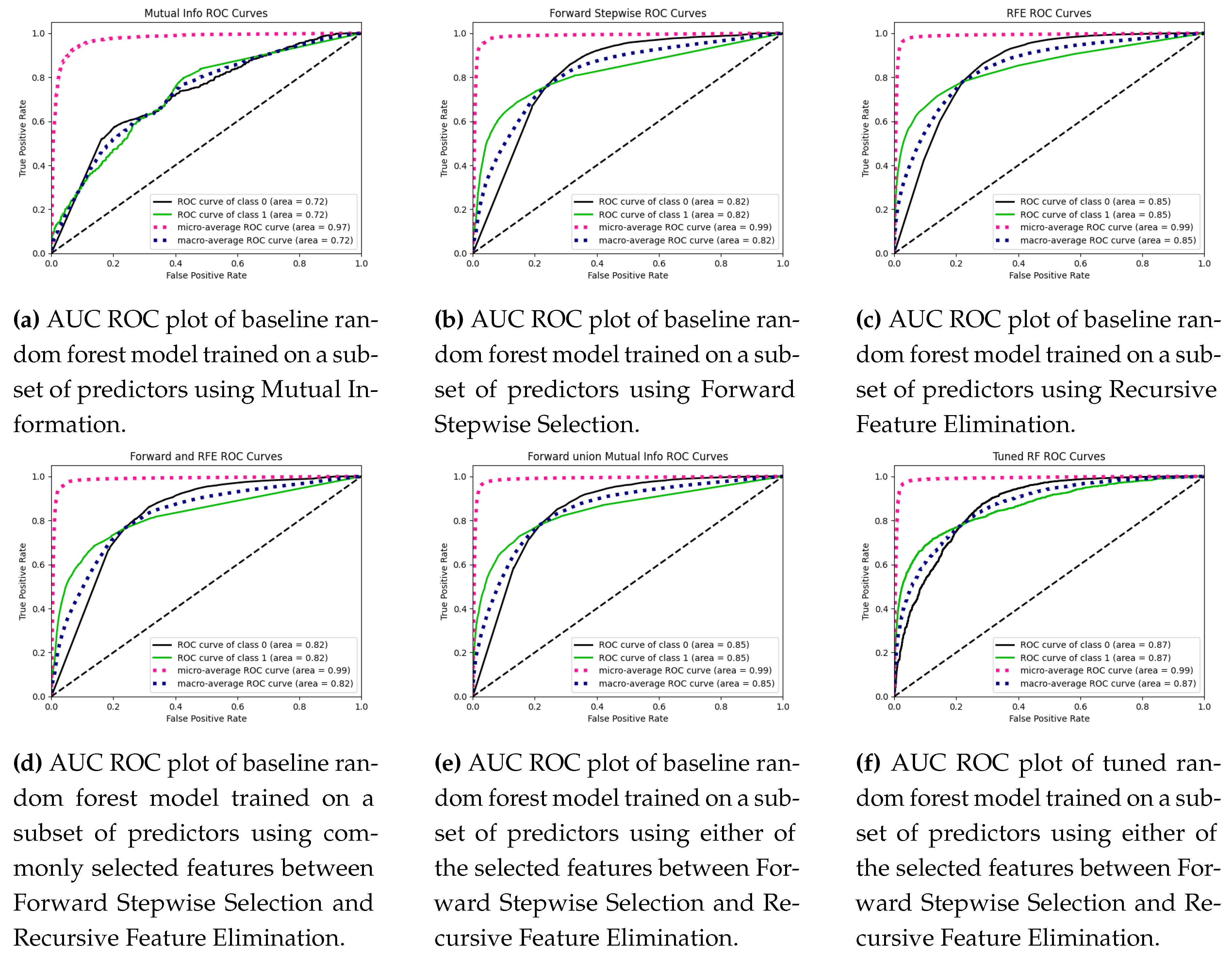
We also select the commonly selected predictors between forward stepwise regression and RFE and the union of the selected features between forward stepwise and mutual information. The motivation behind this is that since some are parametric and some are non-parametric methods of feature selection, we aim to take advantage of both worlds to get a good subset of final predictors. Also, we use standard features between RFE and Forward Stepwise because RFE has more than 3000 features, and taking a union instead would have increased the dimensionality.
Next, we fit a baseline random forest model using the selected features from those five strategies mentioned above and plot the ROC curves to measure the degree of separation the model can perform on the test data. The five mentioned strategies show that the union of selected features between Mutual Information and Forward Stepwise outperforms other methods and is most parsimonious. Hence, we tune the baseline random forest model trained on the data with a subset of predictors selected from standard features between Mutual Information and Forward Stepwise and see a vast improvement in the F1 score, and the AUC score also increases marginally.
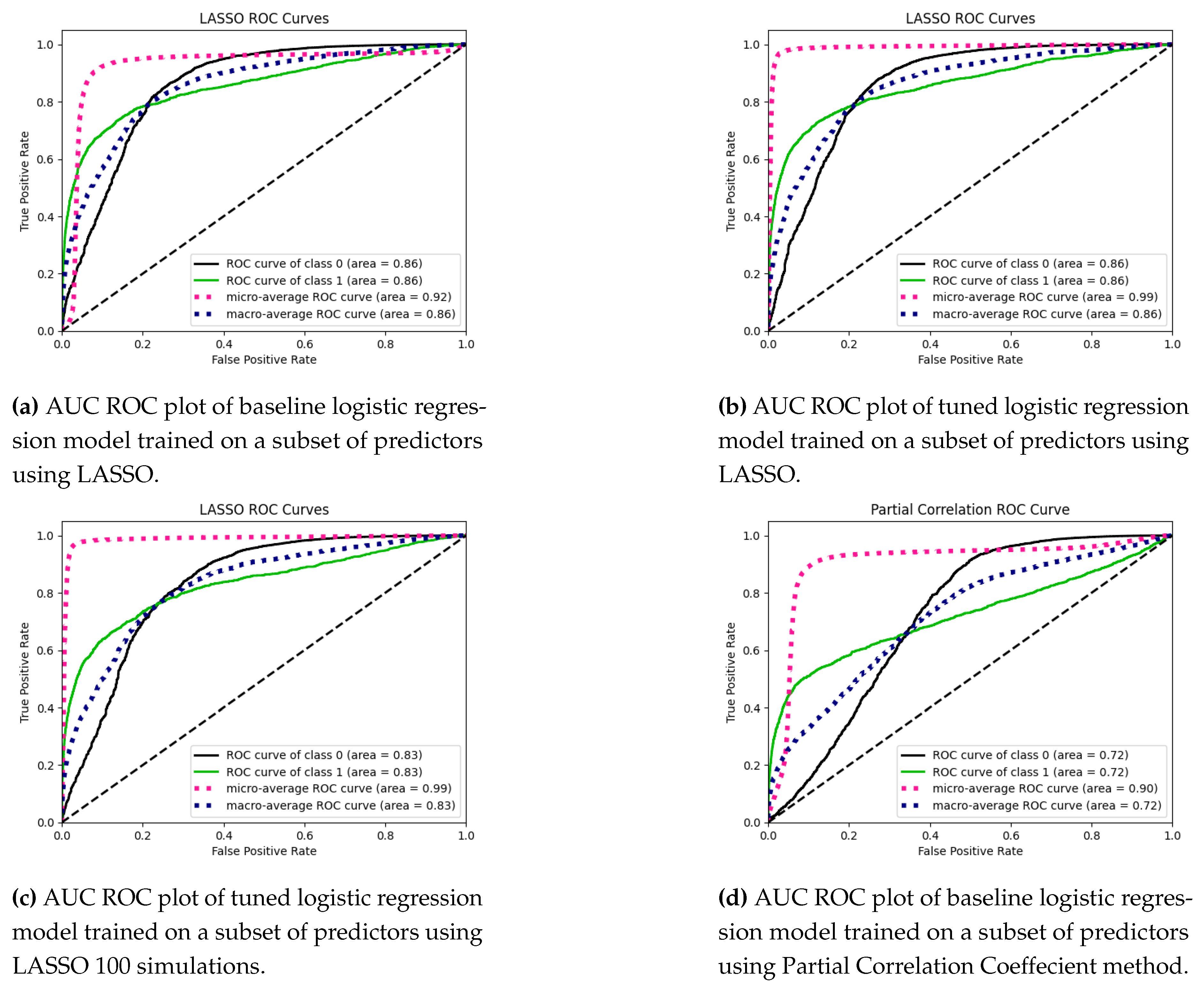
Next, we try using the LASSO and partial correlation coefficient methods to get more optimal subsets of predictors as mentioned below:
LASSO: Lasso [40] is a regression analysis method that performs both variable selection and regularization, but our preference here would be to use it as a feature selection method. LASSO penalizes the sum of the coefficients’ L1 norms, which tends to eliminate the weights of the least important features by shrinking them to zero. This makes the model more interpretable and reduces the curse of dimensionality due to high dimensional feature space. Let X denote the design matrix, Y denote the vector of outputs, and N denote the total samples in the training set. Then, the LASSO optimization is defined as: where denotes the regularization strength. Next, we perform 100 independent simulations of Lasso on a random subset of 2000 samples with replacement from the original training dataset, which is cross-validated on ten folds. Let denote the subset of predictors selected by Lasso during the iteration. The final set of predictors used to evaluate the test set is denoted by
Partial Correlation Coefficient: The partial correlation coefficient quantifies the strength of association between two random variables after accounting for the influence of a set of control variables. This approach aims to mitigate the potential bias introduced by confounding variables when assessing the relationship between two variables using the standard correlation coefficient. Accounting for these confounding factors helps prevent overestimating or underestimating the correlation, providing a more accurate basis for variable selection. The partial correlation coefficient between X and Y given a set of n controlling variables written by is the correlation between the residuals and resulting from regressing and fitting a logistic model on since we have binary labels for Y and not continuous values.
We fit a baseline logistic regression model with the subset of predictors from the LASSO method and then tune the logistic regression model. Similarly, we fit a tuned logistic regression model with the subset of predictors selected from the 100 simulations of the LASSO model. The reason behind just using a selective class of classifiers is that, at this stage, we want to analyze the capabilities of different variable selection methods to give the best sub-optimal set of predictors. This can be done by selecting a classifier and training the same classifier across various various selection methodologies. Similarly, we fit a baseline logistic regression model to the data with the subset of predictors selected using the partial correlation coefficient method.
After exploring the capabilities of all the methodologies, we see that the LASSO with 100 simulations outperforms all others by a considerable margin and with the least number of predictors. This makes the model parsimonious as well. We fit all possible classical machine learning algorithms and evaluate those on the test data. Next, we tune the Random Forest, use the previously tuned Logistic Regression, tune the XGBoost model along with a QDA model, and fit a voting classifier model with soft voting, giving the best F1 and AUC score.
3.3.4. Results
Figure 17 shows the mutual information of the top 50 features selected using the method. Population, material and verbal conflicts between citizens and government, and accidents are the predictors having the highest dependence on the target.
Figure 17.
50 largest Mutual Information gain of the predictors w.r.t to the target variable.
Figure 17.
50 largest Mutual Information gain of the predictors w.r.t to the target variable.
As shown in Table 15, the tuned random forest model with predictors selected from Forward Stepwise ∪ Mutual Information has a better F1 score. The AUC score of the classifier is also the highest, as seen in Figure 18. After we use LASSO, we see that LASSO has a better F1 score of 0.41, which is better than LASSO 100 simulations. However, on the other hand, LASSO 100 simulations are significantly parsimonious compared to LASSO, having only selected 82 features out of more than 7000 predictors.
Table 15.
Evaluation of different variable selection methods on test dataset. Finally, we tune a random forest model using the (Forward ∪ Mutual Information) variable selection method.
Table 15.
Evaluation of different variable selection methods on test dataset. Finally, we tune a random forest model using the (Forward ∪ Mutual Information) variable selection method.
| Method(No. of selected features) |
Class |
Precision |
Recall |
F1 |
Support |
| Mutual Information(50) |
0 |
0.97 |
1.00 |
0.98 |
38181 |
| Mutual Information(50) |
1 |
0.61 |
0.17 |
0.27 |
1416 |
| Forward Stepwise(77) |
0 |
0.97 |
0.99 |
0.98 |
38181 |
| Forward Stepwise(77) |
1 |
0.37 |
0.18 |
0.24 |
1416 |
| RFE(3616) |
0 |
0.97 |
1.00 |
0.98 |
38181 |
| RFE(3616) |
1 |
0.79 |
0.13 |
0.23 |
1416 |
| Forward ∩ RFE(49) |
0 |
0.97 |
0.99 |
0.98 |
38181 |
| Forward ∩ RFE(49) |
1 |
0.36 |
0.18 |
0.24 |
1416 |
| Forward ∪ Mutual Information(117) |
0 |
0.97 |
1.00 |
0.98 |
38181 |
| Forward ∪ Mutual Information(117) |
1 |
0.67 |
0.17 |
0.27 |
1416 |
| Random Forest(Tuned) |
0 |
0.97 |
1.00 |
0.98 |
38181 |
| Random Forest(Tuned) |
1 |
0.73 |
0.21 |
0.33 |
1416 |
Figure 18.
AUC ROC plots of random forest using different variable selection methodologies.
Figure 18.
AUC ROC plots of random forest using different variable selection methodologies.
Figure 19.
AUC ROC plots of logistic regression using LASSO and PCC variable selection methodologies.
Figure 19.
AUC ROC plots of logistic regression using LASSO and PCC variable selection methodologies.
Figure 20 shows the cumulative distribution of all variables’ partial correlation coefficients. This is divided into two parts: variables with significant p-values and those with non-significant p-values, which are in orange and blue, respectively. We use a novel method for selecting the variables using this distribution. The large chunk of coefficients having insignificant p-values are only present between -0.2 and 0.2. Hence, we selected all those variables with an absolute coefficient value of more than 0.25 just to be safe. The partial correlation coefficient does not perform well as it has a low F1 score and has more than 2000 selected features, which makes the model very complex.
We also see the tuning results of logistic regression using LASSO and LASSO 100 simulations variable selection on five-fold stratified cross-validation in Figure 21. The results are divided into two groups with a marginal difference in mean F1 score for each combination of hyperparameters. Still, we can see that some sets have high IQR, which means they cannot generalize well. Hence, we stick to the hyperparameters with the lowest IQR and no significant outliers.
We fit all the classical machine learning models to the data with a subset of predictors selected using the LASSO 100 simulations method and show the results in Table 16. The logistic regression, random forest, and XGBoost perform exceptionally well in this case. The models mentioned above, except random forest, perform better when tuned using Randomised search with 5-fold cross-validation. Also, although the QDA model has poor precision, it has the highest recall, which the other models lack. Hence, we combine the tuned logistic regression, xgboost, baseline random forest, and QDA using a voting classifier with a soft voting strategy, which has the best F1 score of 0.41 with the least possible features. In the previous section, LASSO gave a similar result but with far more features. LASSO 100 simulations with a voting classifier are much more parsimonious, with 82 important predictors. The AUC ROC plot of the voting classifier also reveals that it is strongly superior to all other models, as shown in Figure 22.
Figure 20.
Cummulative distributions of partial correlation coeffecient. The orange color shows the distribution of those having significant p-values.
Figure 20.
Cummulative distributions of partial correlation coeffecient. The orange color shows the distribution of those having significant p-values.
Figure 21.
Hyperparameter tuning results of Logistic Regression using LASSO variable selection.
Figure 21.
Hyperparameter tuning results of Logistic Regression using LASSO variable selection.
Figure 22.
AUC ROC plot of voting classifier with LASSO 100 simulations.
Figure 22.
AUC ROC plot of voting classifier with LASSO 100 simulations.
Table 16.
Performance of various classifeirs on test dataset with the 82 most important predictors using LASSO 100 simualtions.
Table 16.
Performance of various classifeirs on test dataset with the 82 most important predictors using LASSO 100 simualtions.
| Model |
Class |
Precision |
Recall |
F1 |
Support |
| Logistic Regression(Baseline) |
0 |
0.97 |
1 |
0.98 |
38181 |
| Logistic Regression with LASSO(479) |
1 |
0.71 |
0.22 |
0.34 |
1416 |
| Decision Tree(Baseline) |
0 |
0.97 |
0.97 |
0.97 |
38181 |
| Decision Tree(Baseline)) |
1 |
0.27 |
0.32 |
0.29 |
1416 |
| Random Forest(Baseline) |
0 |
0.97 |
1.00 |
0.98 |
38181 |
| Random Forest(Baseline) |
1 |
0.68 |
0.20 |
0.31 |
1416 |
| KNN(Baseline) |
0 |
0.97 |
1 |
0.98 |
38181 |
| KNN(Baseline) |
1 |
0.67 |
0.17 |
0.27 |
1416 |
| Gaussian Naive Bayes(Baseline) |
0 |
0.98 |
0.92 |
0.95 |
38181 |
| Gaussian Naive Bayes(Baseline) |
1 |
0.16 |
0.40 |
0.23 |
1416 |
| SVM(Baseline) |
0 |
0.97 |
1.00 |
0.98 |
38181 |
| SVM(Baseline) |
1 |
0.78 |
0.14 |
0.24 |
1416 |
| QDA(Baseline) |
0 |
0.98 |
0.87 |
0.92 |
38181 |
| QDA(Baseline) |
1 |
0.15 |
0.60 |
0.23 |
1416 |
| XGBoost(Baseline) |
0 |
0.97 |
0.99 |
0.98 |
38181 |
| XGboost(Baseline) |
1 |
0.64 |
0.25 |
0.36 |
1416 |
| Logistic Regression(Tuned) |
0 |
0.97 |
1.00 |
0.98 |
38181 |
| Logistic Regression(Tuned) |
1 |
0.68 |
0.27 |
0.39 |
1416 |
| Random Forest(Tuned) |
0 |
0.97 |
1.00 |
0.98 |
38181 |
| Random Forest(Tuned) |
1 |
0.81 |
0.15 |
0.25 |
1416 |
| XGBoost(Tuned) |
0 |
0.97 |
0.99 |
0.98 |
38181 |
| XGBoost(Tuned) |
1 |
0.62 |
0.27 |
0.38 |
1416 |
| Voting Classifier |
0 |
0.97 |
0.99 |
0.98 |
38181 |
| Voting Classifier |
1 |
0.60 |
0.31 |
0.41 |
1416 |
Table 17.
Initial Evaluation of different variable selection methods on test dataset using Logistic Regression. Finally, we tune a Logistic Regression model using LASSO.
Table 17.
Initial Evaluation of different variable selection methods on test dataset using Logistic Regression. Finally, we tune a Logistic Regression model using LASSO.
| Method(No. of selected features) |
Class |
Precision |
Recall |
F1 |
Support |
| Logistic Regression with LASSO(479) |
0 |
0.99 |
0.92 |
0.95 |
38181 |
| Logistic Regression with LASSO(479) |
1 |
0.24 |
0.66 |
0.35 |
1416 |
| Logistic Regression with PCC(2213) |
0 |
0.98 |
0.91 |
0.94 |
38181 |
| Logistic Regression with PCC(2213) |
0 |
0.17 |
0.50 |
0.26 |
1416 |
| Tuned Logistic with LASSO(479) |
0 |
0.97 |
1.00 |
0.99 |
38181 |
| Tuned Logistic with LASSO(479) |
1 |
0.73 |
0.29 |
0.41 |
1416 |
Our second objective was to analyze how and which predictors play an essential role in deciding whether or not the conflict will be violent. This can help predict violent movements, resulting in the prevention of lives and properties. For this, we use two approaches:
Random Forest Wrapper Feature Importance: A Random Forest comprises a collection of independent decision trees, each consisting of internal nodes and leaves. At internal nodes, features are selected to partition the dataset into subsets with similar responses, using criteria such as Gini impurity or information gain for classification and variance reduction for regression. Feature importance is gauged by how much they decrease split impurity, with the highest decreasing feature chosen for each node. The average impurity reduction for each feature across all trees in the forest determines its importance. This approach is implemented in Scikit-learn’s Random Forest for classification and regression tasks. It is crucial to assess the importance of features relative to one another. The primary advantage lies in computational speed, as all necessary values are computed during training. However, the method favors numerical and high-cardinality categorical features and may need to pay more attention to the importance of correlated features, potentially leading to erroneous conclusions. Figure 23 shows the top 20 most important features from the baseline random forest model. One thing to note over here is that Random Forest thinks that month and year are the most important predictors, which strengthens our initial hypothesis that there are temporal dependencies in the data and also proves that there are some times when the violence is high as we saw in the counts of violence across time. Apart from this, the important predictors are the material and verbal conflicts between citizens, between governments, and between citizens and governments. Although month and year turn out to be most important in the future, we cannot rely on just month and year because, as a single entity, they do not convey any information in the future unseen data. They are probably confounded with some tragic events or a notorious phase that took place in those months and years, which resulted in higher counts of violence.
Figure 23.
Feature importance using ginni impurity of random forest on 82 features selected using LASSO 10 sims.
Figure 23.
Feature importance using ginni impurity of random forest on 82 features selected using LASSO 10 sims.
- 2.
Shapley Additive Explanations: SHAP values (Shapley Additive exPlanations) is a method based on cooperative game theory and is used to increase the transparency and interpretability of machine learning models. Linear models, for example, can use their coefficients as a metric for the overall importance of each feature. However, they are scaled with the scale of the variable itself, which might lead to distortions and misinterpretations. Also, the coefficient cannot account for the local importance of the feature and how it changes with lower or higher values. The same can be said for the feature importance of tree-based models, which is why SHAP is useful for the interpretability of models. Consider a cooperative game with the same number of players as the name of features. SHAP will disclose the individual contribution of each player (or feature) to the model’s output for each example or observation. We only select a random subset of size 100 from the unseen test data because extracting shap values from the whole test data would take a week and is very inefficient. Figure 24 shows the impact of the predictors on the final prediction probability for a single random sample x. Figure 24a shows that non-verbal conflict between citizens is driving the chances of being a violent conflict, as shown in red. Figure 24b shows that although the year has an increasing impact on the chances, the material conflict between citizens and their lags is reducing the chances. This can be interpreted as the conflicts having a temporal dependency, significantly impacting the final predictions. Similarly, Figure 25 shows the stacked version of the impact of the variables year and accident over the entire subset of observations. The sample index is present at the top of the plot. Figure 25a shows that the year mostly positively impacts the predictions due to the red peaks in the plot. There are specific samples for which the year has a negative impact. This can also be seen in the temporal analysis of counts, which clearly shows that some years had a higher count of violent conflicts than others.
Figure 24.
Shap values of a random sample selected from random subset of size 100 from the test data, showing the directional importance of predictors. Red means a positive impact on the base prediction probability making it higher and blue means a negative impact on the base prediction probability making it lower.
Figure 25.
Shap values of the whole subset from test sample showing the directional importance of predictors. Red means a positive impact on the base prediction probability making it higher and blue means a negative impact on the base prediction probability making it lower.
Figure 25.
Shap values of the whole subset from test sample showing the directional importance of predictors. Red means a positive impact on the base prediction probability making it higher and blue means a negative impact on the base prediction probability making it lower.
3.4. Phase IV
Phase I focused on modeling the data using CNN to encode the spatial signals and LSTM to encode the temporal signals. Nevertheless, the performance of the model and its different variations were poor, as the deep neural networks could not model the spatiotemporal imbalanced data well. The following two phases focused more on temporal analysis and generalized feature selection, respectively, which showed significant improvement compared to their predecessors and were less complex than the previous models. The spatial structure of the data has yet to be analyzed explicitly in any of the previous phases. Understanding global and local spatial dependency can help us identify crucial clusters of violent zones that strongly influence neighboring spatial locations. Modeling the global spatial dependency using Tree Boosted Gaussian Process can help us decide if the spatial dependency is insignificant. We can use classical machine learning methods to make inferences. Phase IV analyzes global spatial dependency using global Moran’s I, visualizes the overall distribution of conflicts and local clusters geographically using local Moran’s I, and models the spatial data using GPBoost.
3.4.1. Global Analysis
UUsing only the first file without lags, we merge the geographical coordinates data to find the distance between different spatial locations. Using the unique location IDs for each spatial location, we calculate the distance matrix using geodesic distance between every pair of spatial locations. Treating the distance matrix as features and aggregated conflict counts as a response, we divide the data into training and test using a 70:30 split and train a K Nearest Neighbors(KNN) model on the train data to identify the optimal number of neighbors, a spatial location is related to. Using the test set, we conclude that k=2 has the least MAPE. This means that a given spatial location is spatially related to its two nearest neighbors. We use the optimal value of k to create a weight matrix W such that: , where is the distance between a spatial location and its second nearest neighbor.
Using the weight matrix W, we calculate the global Moran’s I. For the conflict data, the observations are related spatially. We also have a temporal relationship for each spatial location, so we cannot directly apply the classical Moran index. In order to quantify the spatial autocorrelation of a spatiotemporal series, we measure the temporal trend proximity and the magnitudes deviation, as stated by [12] to extend the index for spatiotemporal data. The temporal trend proximity is evaluated using time-lagged cross correlation between the temporal series of a location and the series of global mean values, given by and magnitudes deviation is measured using the deviation in accumulated volumes between the location and the series of global mean values, given by (). Then, the temporal variance and accumulative volume are integrated to set up a deviation measure . Finally, the global Moran’s index for spatiotemporal data is given as . Using the method described above, we calculate the global Moran’s index which comes out to be 0.11. As shown by [31], using a set of equally like random permutations of n events, we can calculate the moments of under the null hypothesis, which can be used to calculate the Z score and hence the p-value, which comes out to be .
3.4.2. Local Analysis
Moran’s index can also find the local clusters or clusters among the data. Local clusters can be classified into four types: HH represents high values surrounded by high values, LL represents low values surrounded by low values, HL represents high values surrounded by low values(hotspots), and LH represents low values surrounded by high values(coldspots). As we can see in Figure 26, the regions near Mexico City, Guadalajara, Monterrey, and Merida are some of the few places having clusters of conflicts. Using the same values calculated before, we compute the local Moran’s index . For the scope of this section, we are only interested in finding the clusters having at least a single high-type region, i.e., HH, HL, or LH. We then analyze the top 15 locations having the largest Moran index.
Starting with the original data, we filter out the locations with the 15 largest indexes for further analysis. Then, we aggregate the data on each spatial location, giving us a time series ranging from 2003 to 2020. Analyzing the temporal signals of these clusters can give us an understanding of the differences or similarities between the global set of locations and these locations. We use the log transform to stabilize the variance. Differencing does not yield any improvements, as there is a significant dip from 2012 to 2014. Using the ACF and PACF plot, we see that the ACF does not cut off, whereas the PACF cuts off after lag 1. So, we fit an AR(1) model along with other ARMA models to the data and thus infer that the BIC of the AR(1) model is the least, which is 41. The model diagnostics show that the AR(1) model is a decent fit on the series if not a very good fit. The ACF, PACF, and LB statistics show no autocorrelation among the residuals. The QQ plot of the residuals shows that they are not normally distributed and have a light tail. This tells us that the temporal signals of these clusters are, in fact, very similar to the global conflict data, and on a spatial level, they differ when the local spatial dependency is analyzed using Moran’s index. Figure 27 shows the presence of various clusters having either high influence on their neighbors or being high conflict zones themselves. As we can see from the plot, the regions having clusters are consistent with Figure 26, which shows the high presence of conflicts near Mexico City, Merida, and Monterrey. We can also see some less conflict-prone regions like Sinaloa and Oaxaca popping up in the plot. These are those regions that have low violent conflicts but are surrounded by zones of high conflicts.
Figure 26.
This plot shows the occurrences and spread of conflicts in Mexico across time. The red dot represent the violent cases(1) and the green ones represent the non violent cases(0).
Figure 26.
This plot shows the occurrences and spread of conflicts in Mexico across time. The red dot represent the violent cases(1) and the green ones represent the non violent cases(0).
Figure 27.
This plot shows local cluster centers of conflicts, which are either HH, HL, or LH type.
Figure 27.
This plot shows local cluster centers of conflicts, which are either HH, HL, or LH type.
3.4.3. Spatial Modelling
Gaussian Processes are one of the most widely used methods for modeling spatial data, mainly because of their ability to make probabilistic predictions; they can be seen as probable prior models that can be effectively used to model spatial correlation among the samples. However, if the spatial data has additional covariates, the standard spatial Gaussian process assumes a linear relationship between the covariates and response, thus introducing bias in the model. Boosting techniques are non-parametric methods that create an ensemble of uncorrelated trees. They differ from random forests because they build upon the previous errors by giving more weight to those examples using some strategy. However, they disregard any potential spatial correlation among samples, produce discontinuous spatial predictions, and do not consider any reasonable prior information about two adjacent locations.
GPBoost [39] is an algorithm that combines the strengths of Gaussian processes and tree boosting methods, which iteratively learns the covariance parameters of the Gaussian process and adds a new tree using the gradient boosting step to account for the spatial correlation in the data. It is assumed that , where y is the response variable, X contains the predictor variables with F being a potentially non-linear function, is a Gaussian process where S denotes the spatial locations and is the error term.
We aggregate the data on location, thus making it a spatial series followed by thresholding the response , where 1 means there is at least a single violent conflict in the location over time. Next, we split the data into train and test with stratification using a 70:30 split ratio, where 70 % goes into train and the rest into the test. We train the GPBoost model on the training data(X) and the geographical coordinates(S) using Bernoulli probit likelihood since we have a binary response. After the model is trained, we get the predictions on the test set by thresholding the probability values that the model returns as . Using these predictions, we evaluate the model using the F1 score and AUC ROC score to compare the model with previous phases.
Figure 28 shows the AUC ROC score of the GPBoost model, which is evaluated on the test set. The AUC of the model is just above 50% with an F1 score of 20%, which is very low compared to the Voting Classifier from Phase III. The autocorrelation analysis using global and local Moran’s Index and the spatial GPBoost model tells us that the dataset does not have significant global spatial dependency among the samples. This means that, without loss of generality, the dataset can be treated as a tabular dataset without considering the spatial relationship between the locations.
Figure 28.
AUC ROC curve of GPBoost model on the test set.
Figure 28.
AUC ROC curve of GPBoost model on the test set.
4. Model Comparison
When solving machine learning problems, researchers and practitioners often have to choose between classical machine learning models and neural network models. Both approaches have their strengths and weaknesses, and the decision depends on several factors, such as the complexity of the problem, the availability of data, computational resources, interpretability requirements, and performance expectations. This section will compare classical machine learning and deep neural network models to provide insights into their characteristics.
Model Complexity: Traditional machine learning algorithms like decision trees and logistic regression typically feature simpler architectures than neural networks. These models operate on predefined algorithms and mathematical formulas to generate predictions based on input features. They offer easier interpretability, making them suitable for scenarios where understanding the model’s inner workings is crucial, such as finance or healthcare, or in cases where identifying key variables contributing to anti-government conflicts is a secondary objective. In contrast, neural network models consist of interconnected layers of artificial neurons that can directly learn complex patterns and relationships from the data. While neural networks can capture intricate nonlinearities and potentially achieve higher predictive accuracy, their opaque nature often poses challenges in interpreting and comprehending the model’s internal mechanisms.
Feature Engineering: Classical machine learning models often require manual feature engineering, where domain experts select and engineer relevant features to represent the problem effectively. This process can be time-consuming and requires expertise in the specific domain. However, with well-engineered features, classical models can perform well even with limited data. Neural network models, particularly deep learning architectures, have the advantage of automatically learning features from raw data. They can extract meaningful representations and hierarchical features through multiple layers of abstraction. This feature learning capability reduces the need for manual feature engineering, making neural networks more suitable for scenarios with large and complex datasets.
Scalability and Computational Resources: Classical machine learning models are generally more computationally efficient than neural network models, especially for smaller datasets. Training a classical model requires less computational power and memory, enabling faster iterations and experimentation. This advantage makes them useful when computational resources are limited or time constraints are critical. In contrast, neural network models, especially deep learning models, are computationally demanding and often require powerful hardware, such as GPUs or specialized hardware accelerators, to train efficiently. They excel when dealing with large-scale datasets and complex problems, but this scalability comes at the cost of increased computational resources and longer training times.
Generalization and Performance: Classical machine learning models can perform well when the dataset is relatively small and the problem separates classes or features. These models are less prone to overfitting and can be generalized effectively. They are also suitable for problems with high-dimensional but sparse feature spaces. Neural network models, with their ability to learn intricate patterns and nonlinear relationships, excel in tasks where the data is abundant and the problem is highly complex. However, they are more prone to overfitting, especially when the dataset is limited. Regularization techniques, such as dropout and weight decay, are often employed to mitigate overfitting in neural networks.
Finally, we quantify these contrast measures using model performance between the classical methods and neural network models. Table 18 compares the neural network models used in the first phase and baseline classical machine learning algorithms. It can be seen that the ensemble-based models(Random Forest and Gradient Boosting) outperform all the other models in terms of F1 score. If we talk about complexity, the gradient boosting algorithm is the most complex, which takes around 1042 unit times for training. On the other hand, KNN has the least training time, within a unit time, but is most expensive during evaluation. Because KNN is essentially an algorithm that stores the data during the training phase, thus creating a map or database. During the testing phase, it calculates the distance between the new unseen record and all previously stored records, making it very complex.
Table 19 compares the neural network models and classical methods with ensembles used in the second phase with just two lag files. The classical ensemble-based voting classifiers are again outperforming the neural networks, although there is no significant improvement in the ensemble models compared to phase one. The best-performing neural network model has a lower F1 score in the second phase than the first. Similar to the previous phase, the neural networks model has a very low precision but the highest recall among others, meaning they have many false positives. Voting Classifier 2 outperforms all the other models because all the base classifiers are non-parametric. There is a difference in the distribution of the majority and minority classes between the neural networks and the classical models. Although the minority class count remains the same, the count of majority classes is higher in neural network-based models. This is because we randomly add a municipality from the municipalities with just the majority class in the undersampled dataset. This makes the municipalities count in the undersampled data 648 for neural networks but only 647 for the classical methods. We do this to get an even count divisible by three so that the architecture of the neural network is feasible.
In the final phase of the research, we use various feature selection methodologies, out of which LASSO stands out by a considerable margin in terms of performance and complexity. A novel variation of LASSO, referred to as LASSO 100 sims in this paper, was used to make the LASSO more parsimonious and reduce the number of non-zero predictors to 82 from 479. As in the previous phases, the neural networks are still struggling to break even, and the magnitude of the difference between the performance of neural networks and classical methods has increased colossally, as shown in Table 20. The poor performance of the neural networks might lead to the conclusion that there is no statistically significant spatial autocorrelation between the conflicts because, on the same data, the classical methods can perform better by a considerable margin without the spatial structure. The distribution of classes in classical methods is different from neural networks because we use random stratified splitting for classical methods, thus ignoring the spatiotemporal auto-correlation and assuming it is a tabular dataset.
Table 18.
Phase 1 comparison of classical machine learning models with deep neural networks showing the poor performance of neural networks. The classical methods are trained on original data with all the municipalities.
Table 18.
Phase 1 comparison of classical machine learning models with deep neural networks showing the poor performance of neural networks. The classical methods are trained on original data with all the municipalities.
| Model |
Precision(1) |
Recall(1) |
F1(1) |
Training Time (sec) |
Evaluation Time (sec) |
Support distribution |
| CNN+LSTM |
0.00 |
0.31 |
0.01 |
569 |
4 |
132377(0) vs 301(1) |
| CNN + LSTM (Undersampled) |
0.01 |
0.38 |
0.02 |
227 |
3 |
132377(0) vs 301(1) |
| CNN + LSTM (Concatenation with Undersampling) |
0.01 |
0.78 |
0.02 |
249 |
3 |
132377(0) vs 301(1) |
| CNN + LSTM (2 Independent Datasets with Undersampling) |
0.03 |
0.34 |
0.05 |
192 |
1 |
132377(0) vs 301(1) |
| Logistic Regression |
0.13 |
0.02 |
0.03 |
20.92 |
0.11 |
132377(0) vs 301(1) |
| Decision Tree |
0.04 |
0.24 |
0.06 |
70.93 |
0.21 |
132377(0) vs 301(1) |
| Random Forest (Un-weighted) |
0.55 |
0.16 |
0.25 |
241.41 |
4.17 |
132377(0) vs 301(1) |
| KNN |
0.11 |
0.23 |
0.15 |
0.22 |
788.92 |
132377(0) vs 301(1) |
| Naive Bayes |
0.02 |
0.51 |
0.04 |
3.41 |
1.29 |
132377(0) vs 301(1) |
| Gradient Boosting |
0.30 |
0.22 |
0.25 |
1041.19 |
0.64 |
132377(0) vs 301(1) |
Table 19.
Phase 2 comparison of classical machine learning models with deep neural networks showing the poor performance of neural networks. The classical methods are trained on undersampled data with 647 municipalities having both the majority and minority class.
Table 19.
Phase 2 comparison of classical machine learning models with deep neural networks showing the poor performance of neural networks. The classical methods are trained on undersampled data with 647 municipalities having both the majority and minority class.
| Model |
Precision(1) |
Recall(1) |
F1(1) |
Training Time (sec) |
Evaluation Time (sec) |
Support distribution |
| CNN + LSTM (Concatenation with Undersampling) |
0.02 |
0.63 |
0.03 |
209 |
3 |
42375(0) vs 393(1) |
| CNN + LSTM (2 Independent Datasets with Undersampling) |
0.01 |
0.74 |
0.02 |
234 |
3 |
42375(0) vs 393(1) |
| Logistic Regression |
0.19 |
0.12 |
0.15 |
5.22 |
0.06 |
42309(0) vs 393(1) |
| Decision Tree |
0.04 |
0.23 |
0.07 |
11.22 |
0.08 |
42309(0) vs 393(1) |
| Random Forest (Un-weighted) |
0.36 |
0.18 |
0.24 |
45.08 |
1.35 |
42309(0) vs 393(1) |
| KNN |
0.14 |
0.17 |
0.15 |
0.28 |
40.49 |
42309(0) vs 393(1) |
| Naive Bayes |
0.04 |
0.45 |
0.07 |
0.90 |
0.38 |
42309(0) vs 393(1) |
| Gradient Boosting |
0.26 |
0.22 |
0.24 |
116.62 |
0.29 |
42309(0) vs 393(1) |
| Voting Classifier 1 (Hard) |
0.34 |
0.21 |
0.26 |
37.68 |
2.50 |
42309(0) vs 393(1) |
| Voting Classifier 2 (Hard) |
0.38 |
0.19 |
0.25 |
228.91 |
6.58 |
42309(0) vs 393(1) |
| Voting Classifier 3 (Hard) |
0.04 |
0.45 |
0.07 |
11.07 |
1.99 |
42309(0) vs 393(1) |
Table 20.
Phase 3 comparison of classical machine learning models with deep neural networks where neural networks continue to perform poorly. The classical methods are trained on whole data with 647 municipalities with 7232 predictors having both the majority and minority class. The neural networks and the voting classifier are trained on 82 predictors from the union of predictors from 100 independent LASSO simulations.
| Model |
Precision(1) |
Recall(1) |
F1(1) |
Training Time (sec) |
Evaluation Time (sec) |
Support distribution |
| CNN + LSTM (Concatenation with Undersampling) |
0.01 |
0.65 |
0.02 |
105 |
1 |
42375(0) vs 393(1) |
| CNN + LSTM (2 Independent Datasets with Undersampling) |
0.03 |
0.36 |
0.05 |
50 |
1 |
42375(0) vs 393(1) |
| Logistic Regression |
0.67 |
0.27 |
0.38 |
44.68 |
1.43 |
38181(0) vs 1416(1) |
| Decision Tree |
0.27 |
0.30 |
0.29 |
557.99 |
1.67 |
38181(0) vs 1416(1 |
| Random Forest (Un-weighted) |
0.82 |
0.17 |
0.28 |
497.22 |
4.97 |
38181(0) vs 1416(1 |
| KNN |
0.55 |
0.11 |
0.18 |
17.22 |
420.84 |
38181(0) vs 1416(1 |
| Naive Bayes |
0.15 |
0.34 |
0.20 |
14.34 |
5.15 |
38181(0) vs 1416(1 |
| Gradient Boosting |
0.66 |
0.27 |
0.39 |
1120.34 |
2.69 |
38181(0) vs 1416(1) |
| Voting Classifier with LASSO 100 sims (Soft) |
0.60 |
0.31 |
0.41 |
34.24 |
1.39 |
38181(0) vs 1416(1) |
| Voting Classifier with LASSO complete (Soft) |
0.63 |
0.33 |
0.43 |
111.96 |
2.90 |
38181(0) vs 1416(1) |
5. Algorithm
The following algorithm describes the stepwise process to model the event-type spatiotemporal datasets followed by the extraction of a set of important features.
|
Algorithm 1: Deep learning STDM
|
-
Require:
, -
Ensure:
, ▹ T = time axis, S = spatial axis, P = feature space |
| |
1. Divide . denotes training set, denotes validation set and denotes test set.
2. Divide the data into batches of size b such that where and so on for validation and test dataset.
3. Initialise a deep NN model with CNN layers followed by LSTM layers, keeping the input and output shape as desired. is the set of hyperparameters that define the neural network model consisting of initialisers, number of filters, kernel size, and so on.
4. Train the model on the . Use the validation set to tune and get the optimal hyperparameters .
5. Train the fine tuned model on the whole dataset .
6. Get the prediction probabilities . Using the decile method as shown above, find the lower threshold of the decile having the largest KS value, given by .
7. Using as threshold, classify the predicted probabilites as 1 or 0 using .
8. Plot the ROC curve using and and the confusion matrix as well to evaluate the model predictions.
9. If the results are not as desired go to step 4 and re-tune the model using a more exhaustive strategy, for eg: using grid search on a large number of values. (Note: This might be more complex and could take more resources).
10. If the AUC score is still very low, go to Algorithm 2.
|
|
Algorithm 2: Finding k temporal lags
|
-
Require:
, -
Ensure:
, ▹ T = time axis, S = spatial axis, P = feature space |
| |
1. If there are any spatial locations having only a single class for all the temporal points, drop those instances then split the data into training, validation and test as defined in Algorithm 1.
2. Aggregate the whole data on time by taking the sum of violence counts for all spatial locations at time t, given by , where is the violence label for spatial location s at time t.
3. Perform variance stabilizing transformations using log transformations, , where is a very small quantity to handle zero counts. Next, stationarize the data differencing, .
4. Plot the ACF and PACF of to estimate the p and q parameters. If both the ACF and PACF cut off at some lags, use hit and trial method to select the model having least BIC. If the model having least BIC comes out to be a MA model, select the best performing AR model.
5. Use the k lags of the selected model to select those many lags of the predictor variables and train the previously defined NN model as well as some classical ML models like Decision tree, Logistic Regression and Random Forest on the training set as defined in Algorithm 1.
6. Tune the best performing model on validation data and refit the tuned model on the entire training + validation dataset.
7. Get the predictions on the test set as described in Algorithm 1. Plot the ROC curve and the confusion matrix. If the AUC score is still not as desired, go to Algorithm 3.
|
|
Algorithm 3: Feature selection and importance
|
-
Require:
, -
Ensure:
, ▹ T = time axis, S = spatial axis, P = feature space |
| |
1. Transpose and in a tabular data format having dimensions as spatial*temporal instances and features, dim(X) = ST*P.
2. Next, perform 100 independent simulations of LASSO on a random subset of 2000 samples with replacement from the original training datatset which is cross validated on 10 folds. The subset size could be increased depending on the availability of computing resources.
3. Let denote the set of predictors having non-zero coefficients from LASSO during the iteration. The final set of predictors used to evaluate on the test set is denoted by .
4. Using as the reduced predictor space, train the NN and the classical ML methods and then tune the top 3 performing models on validation dataset.
5. Selecting the top 3 performing model, train a voting classifier with soft voting on the the whole training + validation dataset, selecting only the features in .
6. Get the predictions using the voting classifier and plot the ROC and confusion matrix.
7. Train a random forest model, if not already used in the voting classifier on the complete dataset and using the feature importance wrapper method, plot the relative feature importance.
|
6. Discussions and Conclusions
We tried several approaches to fit a model to this data as parsimonious as possible using neural network architecture and classical machine learning models with and without feature selection, analyzing the importance of the predictors in classifying the conflicts as violent or non-violent.
We first try to fit a deep learning CNN2D + LSTM model with 3D data with the three axes representing municipalities, time, and features, respectively. We fit different variations of the architecture, but all of them perform poorly. Simultaneously, we also fit a Random Forest model, which performs significantly better. This might be because there are no significant spatial or temporal dependencies in the data, or there might be more noise in the data compared to signals that can be resolved using dimensionality reduction, speaking just from the data perspective. We expect this kind of difference between classical methods and neural networks for tabular datasets because neural networks are overly smooth functions and invariant to rotations for tabular datasets, making them inferior compared to classical methods just for tabular datasets.
We analyze the univariate time series data on the counts of violent conflicts over the years aggregated over the municipalities sampled monthly. We see that the number of violent conflicts dropped significantly after 2012. We also analyzed the temporal dependencies of the violence counts over the years and found that they follow an ARIMA(1,1,0) model. This means the violent counts are only dependent on the last month’s counts and no more. This motivates us to keep only the first two files and drop the rest.
After dropping excess lags, we fit the data using several models. The voting classifier 1 with hard voting outperforms all other methods and performs similarly to the random forest trained on the complete data. This further motivates us to reduce the feature dimensionality to make the model less complex.
We finally use various parametric and non-parametric variable selection methodologies to select the most important variables and thus reduce the noise. Out of all those methods, LASSO outperformed the other methods by a considerable margin. LASSO shrinks all unimportant variables’ coefficients to zero, making it effective for sparse datasets like this. The only issue was that it selected more than 400 features, which was enormous. We randomly selected 2000 samples from training data with replacement, fit the LASSO method 100 times independently, and took the union of all the predictors selected in each simulation. Next, we fit all the models on this subset of predictors. The voting classifier with QDA XGBoost, Random Forest, and Logistic Regression in a soft setting gives us a very similar performance with an F1 score of 0.41 with just 82 features. This is the final model, and we select the random forest sub-model of the voting classifier to analyze the feature’s importance.
Using the random forest feature importance, we see that the demographical variables like accident and material conflicts between citizens and governments and verbal conflicts between citizens and governments are the crucial drivers for conflict. Year and month are shown to be most important, but that may be because they have high cardinality, which is why the Ginni impurity methods think they are important while splitting the node. One issue with this method is that we do not know if the crucial predictors increase the chances of violent conflicts or reduce them. For that reason, we use Shap values, which give that information. We see that the year has mainly positive effects, and accident also has positive effects(red peaks), but for most regions, it has less negative impact(plateau of blue curves).
The generalizability of a model to a different region is a critical aspect, especially when considering the importance of features in predicting outcomes. Feature importance analysis helps identify the key variables contributing significantly to the model’s performance. When extending a model to a different region, assessing whether the identified important features remain relevant and influential across diverse geographical contexts is essential. Robust generalizability relies on the stability of these crucial features in capturing patterns and relationships within the new region. If the model’s important features exhibit consistency and maintain their predictive power in the face of regional variations, it suggests a higher likelihood of successful generalization. However, careful consideration and validation are necessary to ensure the model’s adaptability to the unique characteristics of the new region, as shifts in important features may occur due to environmental, cultural, or economic differences. To summarise, if the predictors like accidents, homicides, and material conflicts remain as crucial as they are in the current scenario when the model is applied to a different region without any significant covariate shift, the model will have similar performance and generalize well for different regions.
We also analyze the spatial structure of the dataset using extended global and local Moran’s autocorrelation index and model the data using GPBoost. The global analysis shows us that the global spatial dependency is very low. Hence, we can disregard the assumption of any significant global spatial dependency among the samples. Following the global analysis, the local analysis highlights the fact that although there might not be a significant global spatial dependency among the samples, there are clusters of regions that have either the potential to spread the conflicts to nearby locations or are just surrounded by locations with high conflicts, classified as HH or LH zones. These zones match the pattern of the actual spatial distribution of conflicts in Mexico. Finally, we model the spatial data using GPBoost, which, when evaluated on the test set, shows us that the model is unreliable for unseen data and cannot generalize well. These analyses point us to one common conclusion, which is the fact that there is no significant spatial dependency present among the samples.
References
- Federico Amato, Fabian Guignard, Sylvain Robert, and Mikhail Kanevski. A novel framework for spatio-temporal prediction of environmental data using deep learning. Scientific reports 2020, 10, 22243. [Google Scholar] [CrossRef]
- Luc Anselin. Local indicators of spatial association—lisa. Geographical analysis 1995, 27, 93–115. [Google Scholar] [CrossRef]
- Luc Anselin, Ibnu Syabri, Oleg Smirnov, et al. Visualizing multivariate spatial correlation with dynamically linked windows. In Proceedings, CSISS Workshop on New Tools for Spatial Data Analysis, Santa Barbara, CA, 2002.
- Sercan Ö Arik and Tomas Pfister. Tabnet: Attentive interpretable tabular learning. In Proceedings of the AAAI conference on artificial intelligence, volume 35, pages 6679–6687, 2021.
- Shao-Kuan Chen, Wei Wei, Bao-Hua Mao, and Wei Guan. Analysis on urban traffic status based on improved spatio-temporal moran’s i. 2013.
- Tianqi Chen and Carlos Guestrin. Xgboost: A scalable tree boosting system. In Proceedings of the 22nd acm sigkdd international conference on knowledge discovery and data mining, pages 785–794, 2016.
- Kyunghyun Cho, Bart Van Merriënboer, Dzmitry Bahdanau, and Yoshua Bengio. On the properties of neural machine translation: Encoder-decoder approaches. arXiv 2014, arXiv:1409.1259. [Google Scholar]
- Andrea Cini, Ivan Marisca, Filippo Maria Bianchi, and Cesare Alippi. Scalable spatiotemporal graph neural networks. In Proceedings of the AAAI conference on artificial intelligence, volume 37, pages 7218–7226, 2023.
- Abhirup Datta, Sudipto Banerjee, Andrew O Finley, and Alan E Gelfand. Hierarchical nearest-neighbor gaussian process models for large geostatistical datasets. Journal of the American Statistical Association 2016, 111, 800–812. [Google Scholar] [CrossRef]
- Jean Dubé and Diègo Legros. A spatio-temporal measure of spatial dependence: An example using real estate data. Papers in Regional Science 2013, 92, 19–30. [Google Scholar] [CrossRef]
- Marco Fraccaro, Søren Kaae Sønderby, Ulrich Paquet, and Ole Winther. Sequential neural models with stochastic layers. Advances in neural information processing systems, 29, 2016.
- Yong Gao, Jing Cheng, Haohan Meng, and Yu Liu. Measuring spatio-temporal autocorrelation in time series data of collective human mobility. Geo-Spatial Information Science 2019, 22, 166–173. [Google Scholar] [CrossRef]
- Anthony C Gatrell, Trevor C Bailey, Peter J Diggle, and Barry S Rowlingson. Spatial point pattern analysis and its application in geographical epidemiology. Transactions of the Institute of British geographers, pages 256–274, 1996.
- Robert C Geary. The contiguity ratio and statistical mapping. The incorporated statistician 1954, 5, 115–146. [Google Scholar] [CrossRef]
- Isabelle Guyon, Jason Weston, Stephen Barnhill, and Vladimir Vapnik. Gene selection for cancer classification using support vector machines. Machine learning 2002, 46, 389–422. [Google Scholar] [CrossRef]
- Valeria Helle, Andra-Stefania Negus, and Jakob Nyberg. Improving armed conflict prediction using machine learning: views+. 2018.
- Zhe Jiang, Shashi Shekhar, Xun Zhou, Joseph Knight, and Jennifer Corcoran. Focal-test-based spatial decision tree learning. IEEE Transactions on Knowledge and Data Engineering 2014, 27, 1547–1559. [Google Scholar]
- Ian T Jolliffe. Principal component analysis: a beginner’s guide—i. introduction and application. Weather 1990, 45, 375–382. [Google Scholar] [CrossRef]
- Nitish Shirish Keskar, Dheevatsa Mudigere, Jorge Nocedal, Mikhail Smelyanskiy, and Ping Tak Peter Tang. On large-batch training for deep learning: Generalization gap and sharp minima. arXiv 2016, arXiv:1609.04836. [Google Scholar]
- Mahdi Khodayar and Jianhui Wang. Spatio-temporal graph deep neural network for short-term wind speed forecasting. IEEE Transactions on Sustainable Energy 2018, 10, 670–681. [Google Scholar]
- Diederik P Kingma and Jimmy, Ba. Adam: A method for stochastic optimization. arXiv 2014, arXiv:1412.6980. [Google Scholar]
- Alexander Kraskov, Harald Stögbauer, and Peter Grassberger. Estimating mutual information. Physical review E 2004, 69, 066138. [Google Scholar] [CrossRef] [PubMed]
- Alex Krizhevsky, Ilya Sutskever, and Geoffrey E Hinton. Imagenet classification with deep convolutional neural networks. Advances in neural information processing systems, 25, 2012.
- Yann LeCun, Bernhard Boser, John Denker, Donnie Henderson, Richard Howard, Wayne Hubbard, and Lawrence Jackel. Handwritten digit recognition with a back-propagation network. Advances in neural information processing systems, 2, 1989.
- Jay Lee and Shengwen, Li. Extending moran’s index for measuring spatiotemporal clustering of geographic events. Geographical Analysis 2017, 49, 36–57. [Google Scholar] [CrossRef]
- Mengzhang Li and Zhanxing Zhu. Spatial-temporal fusion graph neural networks for traffic flow forecasting. In Proceedings of the AAAI conference on artificial intelligence, volume 35, pages 4189–4196, 2021.
- Jian Lian, Xiaojuan Li, Huili Gong, and Yonghua Sun. The spatial pattern analysis of economic growth of jingjinji metropolitan region. pages 1–5, 06 2010.
- Fernando López and Coro Chasco. Time-trend in spatial dependence: Specification strategy in the first-order spatial autoregressive model. 2007.
- Patrick AP Moran. Notes on continuous stochastic phenomena. Biometrika 1950, 37, 17–23. [Google Scholar] [CrossRef]
- David Muchlinski, Xiao Yang, Sarah Birch, Craig Macdonald, and Iadh Ounis. We need to go deeper: Measuring electoral violence using convolutional neural networks and social media. Political Science Research and Methods 2021, 9, 122–139. [Google Scholar] [CrossRef]
- J Keith Ord and Arthur Getis. Local spatial autocorrelation statistics: distributional issues and an application. Geographical analysis 1995, 27, 286–306. [Google Scholar] [CrossRef]
- Karl Pearson. Liii. on lines and planes of closest fit to systems of points in space. The London, Edinburgh, and Dublin philosophical magazine and journal of science 1901, 2, 559–572. [Google Scholar] [CrossRef]
- Idan Porat, Maxim Shoshany, and Amnon Frenkel. Two phase temporal-spatial autocorrelation of urban patterns: Revealing focal areas of re-urbanization in tel aviv-yafo. Applied Spatial Analysis and Policy 2012, 5, 137–155. [Google Scholar] [CrossRef]
- Brian C Ross. Mutual information between discrete and continuous data sets. PloS one 8735, 9, e87357. [Google Scholar]
- David E Rumelhart, Geoffrey E Hinton, and Ronald J Williams. Learning representations by back-propagating errors. Nature 1986, 323, 533–536. [Google Scholar] [CrossRef]
- Olga Russakovsky, Jia Deng, Hao Su, Jonathan Krause, Sanjeev Satheesh, Sean Ma, Zhiheng Huang, Andrej Karpathy, Aditya Khosla, Michael Bernstein, et al. Imagenet large scale visual recognition challenge. International journal of computer vision 2015, 115, 211–252. [Google Scholar] [CrossRef]
- Franco Scarselli, Marco Gori, Ah Chung Tsoi, Markus Hagenbuchner, and Gabriele Monfardini. The graph neural network model. IEEE Transactions on Neural Networks 2008, 20, 61–80. [Google Scholar]
- Xingjian Shi, Zhourong Chen, Hao Wang, Dit-Yan Yeung, Wai-Kin Wong, and Wang-chun Woo. Convolutional lstm network: A machine learning approach for precipitation nowcasting. Advances in neural information processing systems, 28, 2015.
- Fabio Sigrist. Gaussian process boosting. The Journal of Machine Learning Research 2022, 23, 10565–10610. [Google Scholar]
- Robert Tibshirani. Regression shrinkage and selection via the lasso. Journal of the Royal Statistical Society Series B: Statistical Methodology 1996, 58, 267–288. [Google Scholar]
- Christopher K Wikle. Modern perspectives on statistics for spatio-temporal data. Wiley Interdisciplinary Reviews: Computational Statistics 2015, 7, 86–98. [Google Scholar] [CrossRef]
- Svante Wold, Kim Esbensen, and Paul Geladi. Principal component analysis. Chemometrics and intelligent laboratory systems 1987, 2, 37–52. [Google Scholar] [CrossRef]
|
Disclaimer/Publisher’s Note: The statements, opinions and data contained in all publications are solely those of the individual author(s) and contributor(s) and not of MDPI and/or the editor(s). MDPI and/or the editor(s) disclaim responsibility for any injury to people or property resulting from any ideas, methods, instructions or products referred to in the content. |
© 2024 by the authors. Licensee MDPI, Basel, Switzerland. This article is an open access article distributed under the terms and conditions of the Creative Commons Attribution (CC BY) license (https://creativecommons.org/licenses/by/4.0/).
