1. Introduction
Glass and plastic greenhouses have been used for centuries in agricultural production in various forms with the basic function of keeping the plants safe from extreme weather conditions. By this is meant that the plants are growth within the area with controlled atmosphere, where optimum air temperature and humidity are provided, as well as the other processes such as irrigation and plant nutrition. The principle of greenhouses operation consists of an isolated area with transparent film through which the solar radiation provides the lighting within the space on one hand, and on the other hand provides a certain level of heating inside the building. Depending on the location of a greenhouse, in most cases it is necessary to carry out additional heating of the building during the winter months, using any conventional source of energy or renewable energy source to improve the energy efficiency of the building. The problem of greenhouses heating was discussed by many scientists over the past few decades, as these buildings entered into mass use in this part of the European continent [
1,
2,
3,
4,
5].
Greenhouses have long since outgrown their original purpose of space in which it is possible to extend the vegetation of plants throughout the year and grew into serious buildings whose thermal behaviour depends on numerous factors that change stochastically. Nowadays, they are very complex and dynamic thermo-technical and agricultural systems where internal conditions such are inside temperature, relative humidity, sensible and latent heat load are strongly dependent from outside unpredictable climate conditions. This interaction is particularly intense is systems with natural ventilation systems, which from the other side affect on inside concentration of carbon-dioxide (CO2) [
6]. Regarding the heating systems, most of existing studies are focused on renewable energy sources implementation, aiming the increase overall facility energy efficiency and reduce the operational costs [
7]. It is primarily thought on various solar energy active and passive systems (thermal, PV, PV-thermal) and geothermal energy application [
8,
9,
10].
In addition to designing an efficient heating system, it is necessary to design a good ventilation system inside the greenhouse, which must be available throughout the year. Independent from temperature and relative air humidity inside a greenhouse, which must suits the physiological needs of plants, the recommended amount of fresh air needed to meet the required amount of CO
2 that plants require, is a minimum of 2 ACH. In most cases, from the smallest and simplest structure to the complex systems with large areas, this amount of fresh air is provided through natural ventilation in greenhouses, by opening one part of the roof domes. In this case ventilation system is based on single-sided natural ventilation through the opening of one half of the roof dome and depends on numerous parameters of the external atmosphere. Although it can be assumed that the effect of natural ventilation in a building depends on the local wind speed, this fact must be taken with caution because the intensity of natural ventilation depends on the ratio between wind direction and surface normal, and it could easily happen that the entire opening is in leeward. In addition, for safety reasons, a situation in which the domes should be closed must be foreseen because of strong gusts of wind that are usually present at the outside air speed exceeding 35km/h. Considering that during night in the winter season the domes are closed in order to maintain the temperature in the space, in order to provide a stable growth of plants it is necessary to predict an alternative way for continuous ventilation of space. In addition to wind effect, in the case of natural ventilation the ventilation plays an important role due to temperature differences, to which attention should be paid especially in the winter months due to great temperature [
11,
12,
13,
14,
15,
16,
17].
Building thermal behavior numerical modelling and overall system dynamic simulation in well know technique and it is widespread in residential and commercial buildings, but also is attractive in greenhouses. To simulate greenhouse, it is necessary to create a complex model that include all greenhouses mutually dependent variables, while at the same time dependent on the unpredictable outside conditions. These models are generally based on solar radiation processing, main thermal source in facility [
18,
19,
20]. Unsteady state equations numerical can be solved by various available engineering software, like MATLAB [
21], or using various scientific Pyhton modules in machine learning algorithms [
6]. The annual greenhouse heating and cooling demand successfully can be simulated with building energy simulation software such as TRNSYS. Although is primarily developed for residential and commercial multi-zone buildings, Type 56 in TRNSYS efficiently can be used also for greenhouse thermal load design [
22]. Along the standard components, it also possible to develop new components and link them with other simulations tools [
23]. The results obtained from these dynamic simulations cannot be taken as facility thermal behavior in real time, primarily because they are based on pre-processed meteorological data (such in TMY, f.e.). Errors also can be generated by simplifying infiltration and ventilation rate, but generally, models developed by TRNSYS can be used for system optimization and energy efficiency improving in facility as whole.
Different machine learning methods can be usefully applied in greenhouse thermal design [
24,
25], whether are inside air parameters or thermal load calculated. Concept of Deep Learning and Artificial Neutral Networks (ANNs) are well known in agricultural applications like yield and irrigation prediction, plant disease detection, image recognition [
26,
27,
28,
29]. ANNs are used in greenhouses for prediction of microclimatic parameters, producing very remarkable and clear results. Modelling inside air temperature and relative humidity, soil temperature, or energy demand [
30,
31], can be achieved with high accuracy based on outside weather condition. Concept of ANNs is based of signals transferring from the nodes (neurons) of the input layer to the nodes of a “hidden layer”, which are activated according to their power, and finally transferring to the output layer. Model accuracy depends from careful choice of “hidden layer” and neurons number, activation function (“hidden layer” power), and number of variables introduced in network. Sing & Tiwari tested ANNs with one hidden layer with different number of nodes [
32], and after several experiments it was found that network with four nodes showed best results for inside air temperature and relative humidity determination. From the other side, Castañeda & Castaño [
33], created a multilayer perception Neural Network with Levenberg–Marquardt as a training algorithm, which can predict the indoor temperature for winter and summer season.
The present study aims to create a model using artificial neutral networks (ANNs), which can predict greenhouse optimal microclimatic parameters, based on outside temperature and relative humidity, as well as inside air and relative humidity from validated TRNSYS model for existing greenhouse. This method can significantly reduce complex algorithm of creating structure for TYPE 56 in TRNSYS simulation, maintaining necessary results accuracy.
2. Materials and Methods
This study was conducted on a greenhouse in region of Šabac municipality in Serbia. In order to validate both models, TNSYS TYPE 56 and ANNs, various types of data were collected from sensors located in the greenhouse, used for controlling thermal conditions.
2.1. TRNSYS Generalized Thermal Load Model
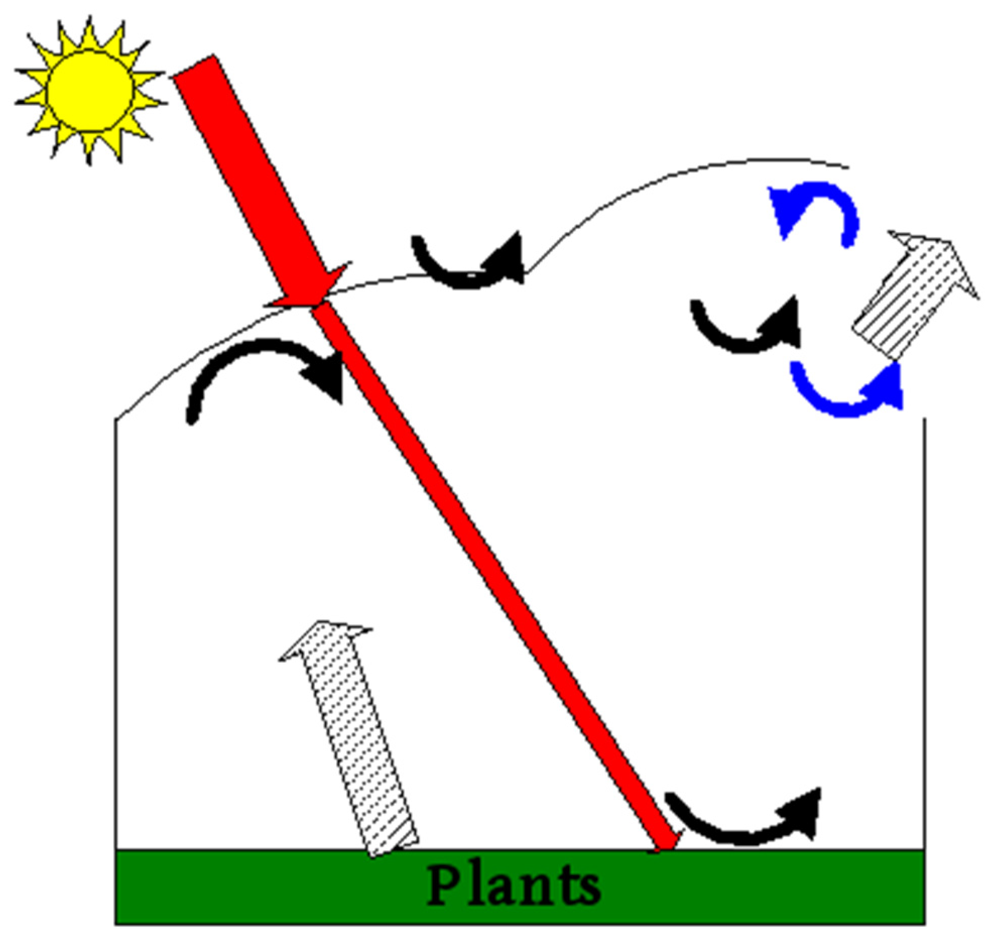
In defining the mathematical model of greenhouse thermal load, tree components play an important role: plants inside the space, air in the building and covering material. Unlike construction buildings, greenhouse has a transparent film whose role is to transmit the solar radiation which is then absorbed by soil and plants. In order to obtain energy flow inside a greenhouse, as shown in
Figure 1, it is necessary to introduce the following preconditions in order to reduce complexity:
- External atmospheric parameters are constant during the time step calculation (hourly values of outside air parameters do not change)
- There is no condensation inside the building, or in the inner surfaces of film
- Change in temperature and relative humidity inside the building is uniform
Heat flux which is transmitted by convection into the air of the building can be expressed by the following equation [
34,
35,
36]:
where
heat flux transmitted by convection from soil into air,
losses due to infiltration,
losses due to ventilation,
thermal load due to internal sources of energy in the building and
heat flux delivered by convection from the walls of the building film into air.
Heat flux which is delivered by radiation to the inner surface of the building film can be represented by the following equitation:
where
is heat flux received by inner surface of the film,
shortwave solar radiation that has passed through the film of the building and directly absorbed by the inner surfaces,
long wave solar radiation that is exchanged between the adjacent inner surfaces of the film and
heat flux from plants towards the inner surfaces of the film of the building.
Energy balance for the film itself can be expressed by:
where
the heat flux that is by convection transmitted from the outside air to the film of the building and
heat flux of radiation between the sky and the outer surface of the covering.
To better determine the dynamic thermal behaviour of the building and monitoring of thermal load dependence due to changes in parameters of external environment, heat transfer coefficients from the outside and inside film of the building are also modelled dynamically. To determine the heat transfer coefficient in the outside film of the building, reduced air speed relative to the normal of the described surface must be determined and in line with [
37]:
surface located in direction of wind flow
surface located in the leeward (oriented opposite to the direction of wind flow)
Where v
l sign represents the local wind velocity towards the observed surface.
Forced convection heat transfer coefficient due to air flow over the outer surface is:
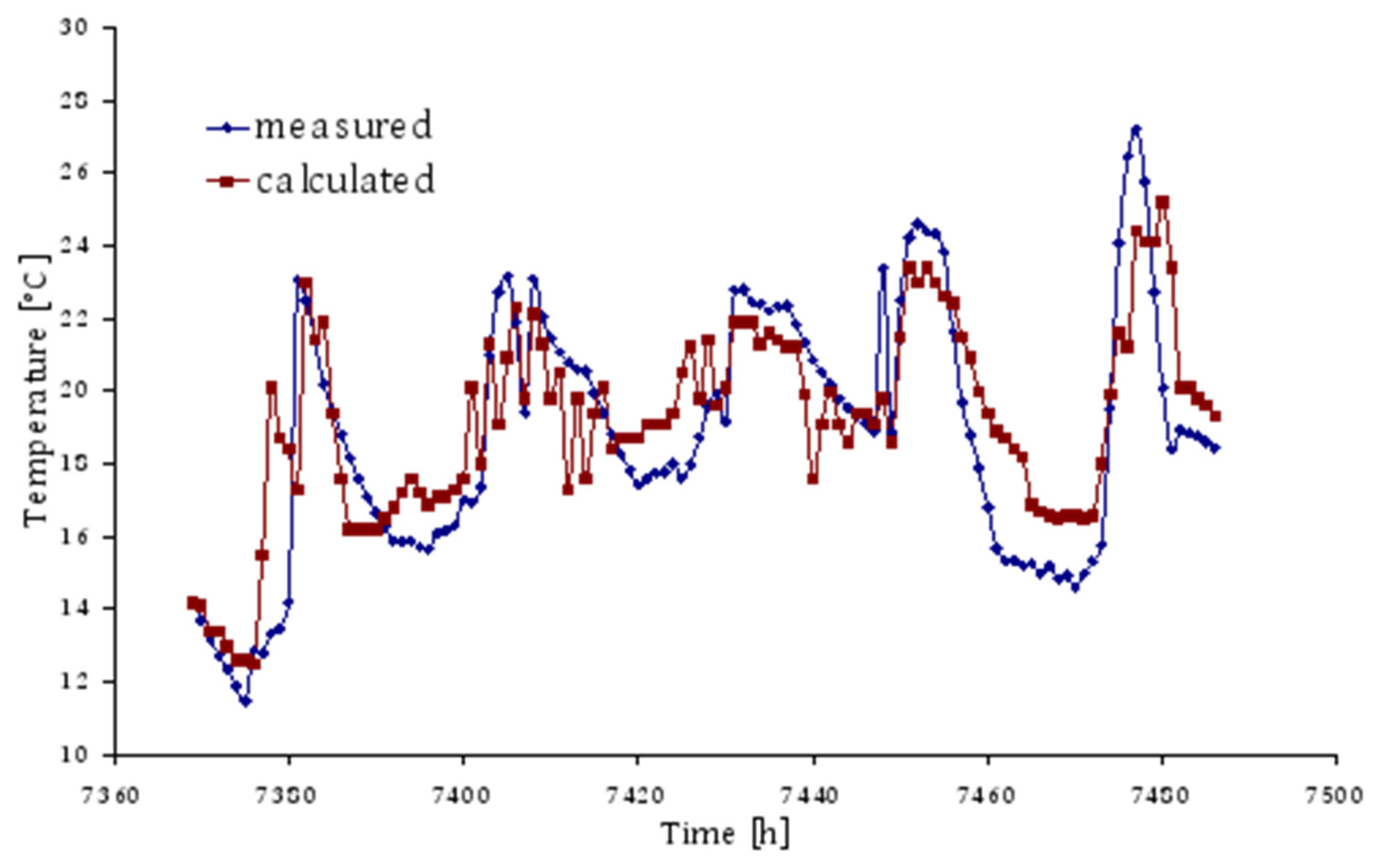
Heat transfer coefficient on the inner film surfaces of the building depends on the combined convection which occurs in the boundary layer directly to the surface and depends on the position, i.e. whether the surface is vertical or horizontal, temperature differences between inner surface and air in the observed zone, as well as on the number of changes of air inside the zone. Validation of the TRNSYS model was carried out on the basis of measured temperature values during the heating period when parameters of the condition of interior space were monitored. In
Figure 2 for five selected days in November a comparison of the air temperature in the house obtained by numerical simulation with the measured values is showed.
Simulation results match well with the measured values and thus it can be concluded that is well positioned and that can be improved by determining the optimal amount of fresh air introduced into the building through natural ventilation in order to create favorable conditions for plant growth during the period from October to May.
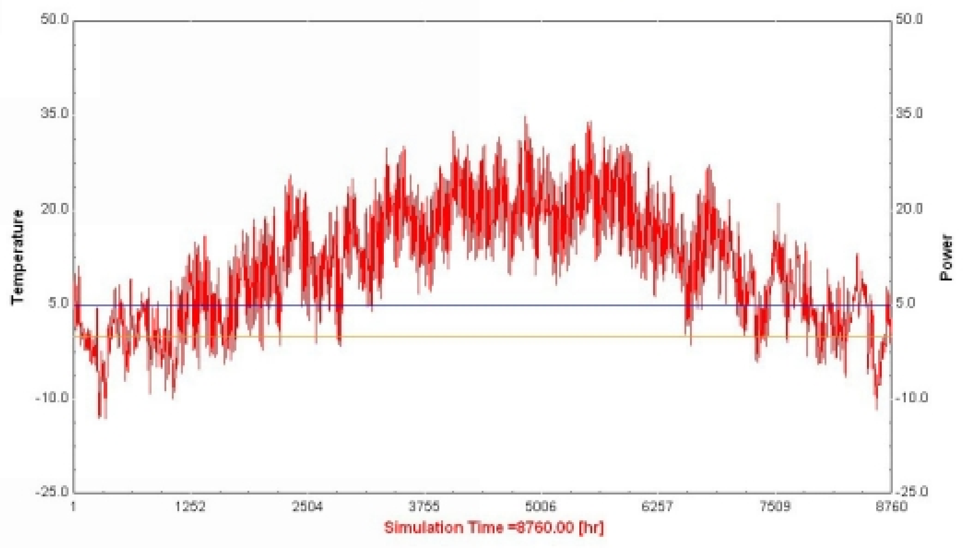
Changes in outside air temperature during the year are shown in
Figure 2. It can be clearly seen that in winter extremely low temperatures are not pronounced, which favorably affects the heat loss especially at night. Minimum temperature according to TMY in the winter is about -10 °C, and the maximum in summer is up to 35 °C.
2.2. Greenhouse Condition
The space inside the greenhouse covers 4.2 ha of area, divided in three parts. One part consists of technical rooms for staff offices, sanitary facilities, two chambers for germination of seeds and two chambers for cooling. In the technical part there is no heating system and temperature is maintained only by solar radiation that passes through the roof domes. A special area with controlled conditions, completely isolated from the rest of the greenhouse, is a part designed for preparation of seedlings in which the required temperature and relative humidity parameters are maintained throughout the year. The rest of the building is divided into four inter-connected areas without any barriers, which further complicates control of plant growth conditions, both in terms of maintaining defined atmospheric conditions and possible isolation of plants from eventual occurrence of diseases. In the central part of the greenhouse, irrigation tanks have been installed as well as pumps which deliver geothermal water for heating and plant nutrition tanks. Vegetable crops are cultivated throughout the year, mostly tomato, pepper and cucumber to a lesser extent and lettuce in the winter.
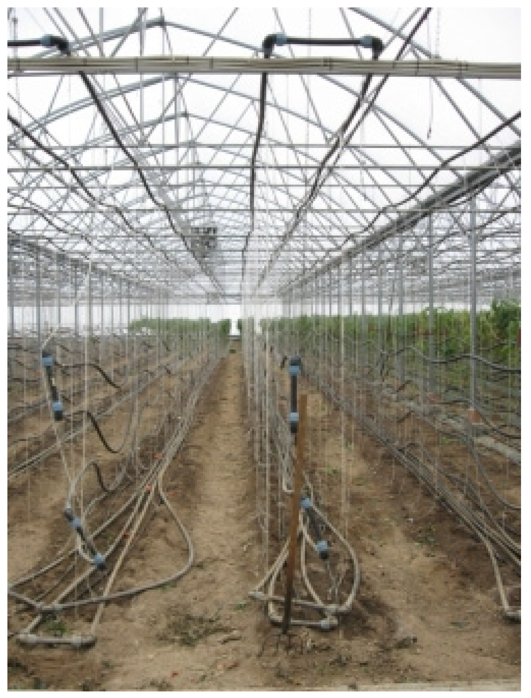
The existing heating system in the greenhouse is made of plastic tubes that are placed vertically on several levels so as to cover the zone where the plants grow (
Figure 4.). The capacity of geothermal energy is 22l/s and temperature of water is 53 °C. When water passes through the heating system in the greenhouse, is cooled to a temperature of 15 °C, and then discharged into the nearby river. Available heat flux for heating is then 2855kW. As part of the heating system, within the plant growing zone of the greenhouse, the tank of 20m
3 in volume is installed, from which the water is transported through pipes to the plant growing zone. Heating system that uses geothermal water covers only necessary plant growing area conditions, which means that during the night, temperature is set to 17°C, and during the day to 20°C.
In the greenhouse there is no system of forced ventilation. Lack of ventilation system has an adverse effect not only on the high temperature which occurs due to solar radiation over the summer, but also on air quality and quantity of CO2 which is necessary for growth and plants development during the day. In the summer, when the problem of high temperatures inside the greenhouse is particularly prevalent, natural ventilation is used for ventilation of the space in which plants are growing. The system is designed so that the domes on the roof aisles are open when the temperature in the greenhouse exceeds a critical given value. The domes are automatically closed when wind speed greater than 35 km/h is detected (due to the structural safety of the roof) or in the case of rainfall and other meteorological disasters. During the summer period, domes are mostly open, and during the winter period, domes are kept open for several hours during the day to ensure intake of fresh air into the greenhouse. According to the recommendations for growing plants in the areas with controlled atmosphere and depending on the area on which plants are cultivated, the minimum flow of fresh air for ventilation only providing sufficient quantities of CO2 should be 2—3 ACH.
The covering of greenhouse comprises of two five-layer foil covers with the air layer of 15cm thickness between them. The shape of the cover is maintained constant by means of overpressure. However, the condition of the foil is relatively bad and irregularly maintained. Therefore, the soiling of the foil reduces the solar flux, and the condition of the entire covering increases the infiltration rate, which is especially bad during the winter nights (despite the relatively high temperatures in the last couple of years), because the heating system fails to achieve the set inner temperature of 20 °C, so it drops to 17°C.
2.3. Artificial Neutral Network Structure
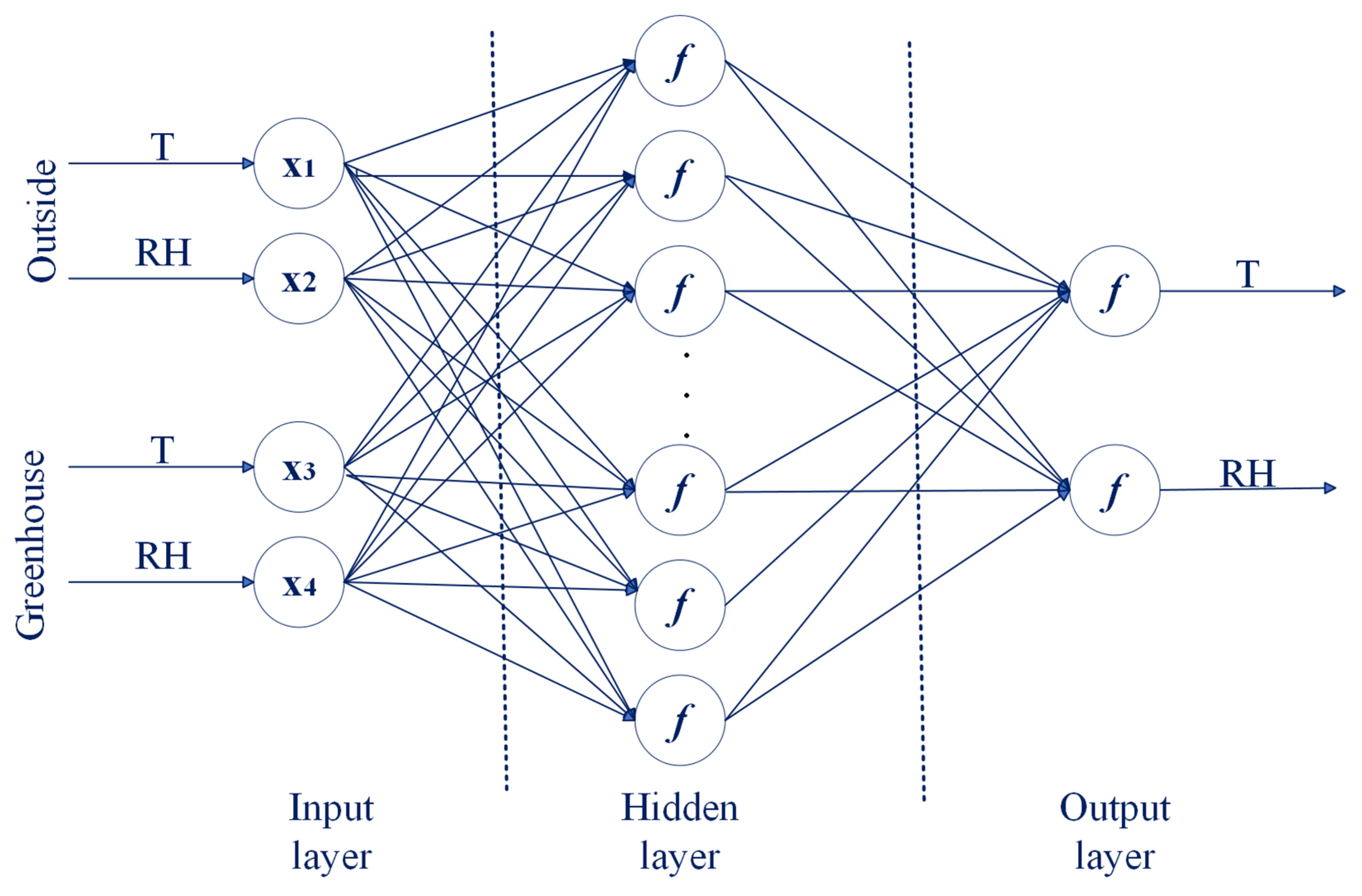
The training and model test set were constructed on the calculated data from TRNSYS simulation and real meteoroogical data for given location. Set of 8760 data was divided in train and test in order of 80: 20. Validation data set were selected from measured data in greenhouse for selected days in heating period. The backpropagation algorithm, which was one of the supervised learning techniques, was used for modeling with the hidden layers to improve the prediction rate of the model (
Figure 5). The ANNs featured outstanding performance since each neuron calculates the weight factor in two stages. The Levenberg-Marqardt algorithm [
38] was used for the learning technique.
Input layer neurons were 4. ANN model is set up on assumption that predicted values of microclimatic parameters–temperature and relative humidity can be improved with real outside conditions. Considering the fact that greenhouses thermal load structure is much more complex than residential building’s due to specific internal gains, ANN model aims to predict microclimatic parameters for specific facility in a simpler way. Output layer neurons were 2–optimal inside temperature and relative humidity. Number of hidden layers and neurons are important factor for model accuracy. Similar researches are mainly based on one hidden layer with number of neurons determined from input and put neurons sum [
30] or based on array of n/2, n, 2n, 2n+1 [
39]. In the study presented in this paper, optimization of the number of neurons, learning rate and number of epochs was carried out in order to find the optimal model that will have the best accuracy and the least losses compared to the initial model. The choice of model is shown in
Table 1.
Due to the reason that ANN model validation was not performed only from the origin data set, but also on the basis of measured real data greenhouse data, the performance measure is given by the linear correlation coefficient, the coefficient of determination, the mean absolute error and the mean square error [
32]. The reason for the double validation lies in the fact that the original data set was also formed on the basis of predictions obtained from the TRNSYS simulation, so the goal was to show how good both prediction models are.
The performance measure is usually given by the linear correlation coefficient (r), coefficient of determination (R2), mean absolute error (MAE) and root mean square error (RMSE):
where, ŷ is predicted value, y is measured value, y is the mean of measured variables and n is the number of samples.
3. Results and Discussion
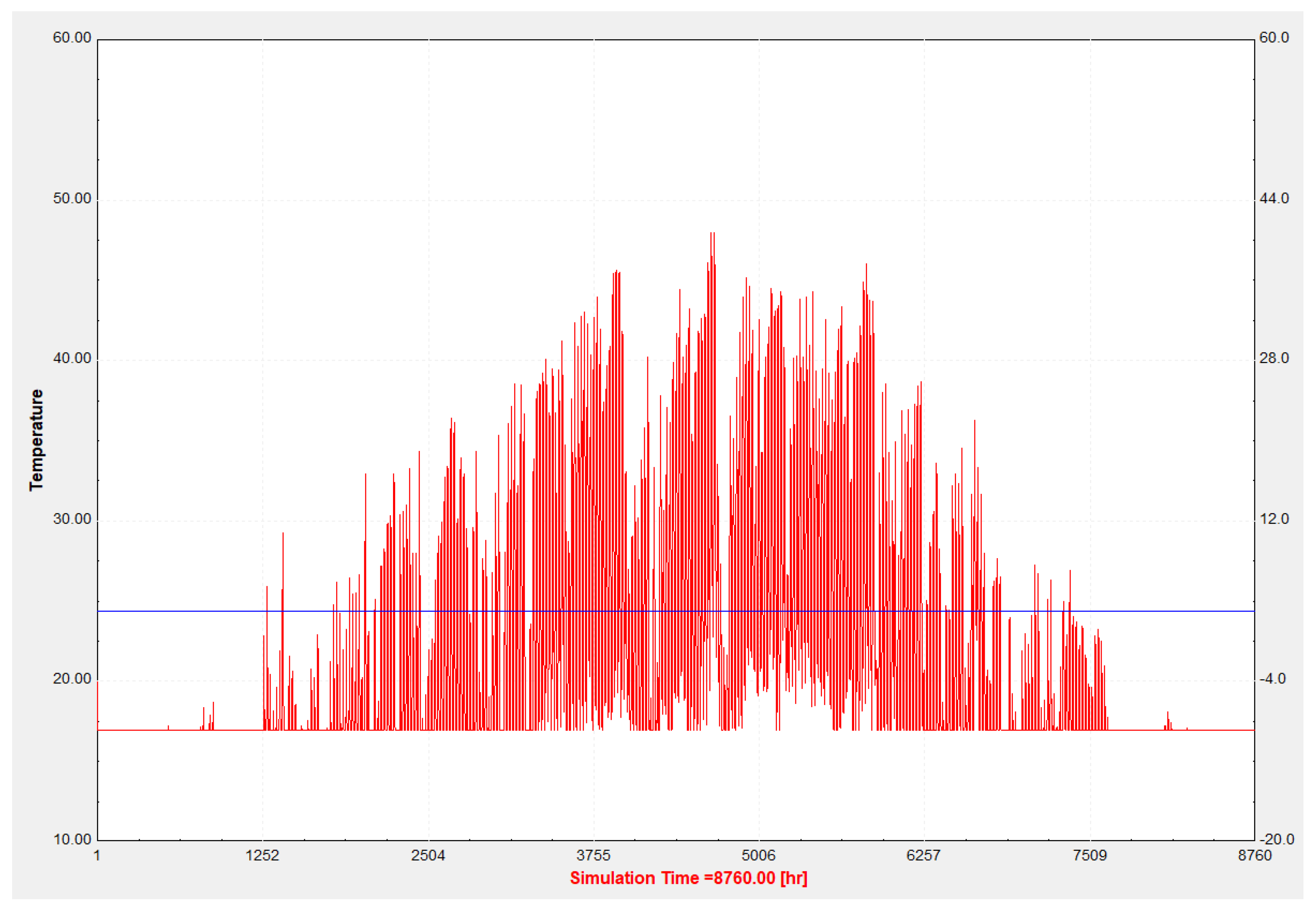
TRNSYS model dynamic simulation for the described object was performed according to the description from Chapter 2.1. The model itself, as it was explained earlier, is very complex and implies a precise definition of the object as a whole: covering, heating system, ventilation, air conditioning, infiltration and internal load. Compared to standard similar simulations, the simulation of the thermal load of the greenhouse is much more complex. The temperature inside the room is the result of complex connections between quantities that change stochastically, such as parameters of the external environment, and conditions inside the object that are dependent on the external environment. Exactly because of this, the goal of this paper is to show that a good ANN model can be created based on the predicted values. The change of the temperature obtained by TRNSYS simulation is shown in
Figure 6.
In the heating period, the TRNSYS model showed a good correlation, which was mentioned earlier. The high temperatures that appear in the model during the summer period are the result of the absence of a mechanical ventilation system. With the minimum adjustments of ACH, the temperatures in the summer period deviate from the measured values in the greenhouse, which is a consequence of lifting the side panels, in order to increase the air flow and reduce the internal temperature.
The model structure was a multi-layer perceptron network with only one hidden layer containing neurons with a hyperbolic tangential activation function and an output layer with two neurons with a linear activation function. In order to define the optimal ANNs model, varying the number of neurons in the hidden layer, the value for the learning rate and the number of epochs, as shown in
Table 1.
Table 1.
The chosen models in simulations with relevant parameters.
Table 1.
The chosen models in simulations with relevant parameters.
| Model |
ANNs neurons
sheme |
Learning rate |
Epoch |
| M01 |
4 - 2 - 2 |
0.02 |
200 |
| M02 |
4 - 3 - 2 |
| M03 |
4 - 4 - 2 |
| M04 |
4 - 5 - 2 |
| M05 |
4 - 6 - 2 |
| M06 |
4 - 7 - 2 |
| M07 |
4 - 8 - 2 |
| M08 |
4 - 9 - 2 |
| M09 |
4 - 10 -2 |
| M10 |
4 – 6 – 2
|
0.018 |
200 |
| M11 |
300 |
| M12 |
0.0079 |
200 |
| M13 |
300 |
The first step in determining the best model training algorithm is determining the number of neurons in the hidden layer according to the previously described settings of the entire ANN model. The results of this training are shown in
Table 2. Using the RMSE algorithm for value analysis, the M05 model showed the best values of the RMSE and mean absolute error (MAE), where the temperature difference between the initial data and the data predicted by the model was 0.4083 and 0.1670, respectively. The values for relative humidity were relatively uniform, so the M05 model was selected for fine-tuning, by varying the value of the learning rate and the number of epochs, which is shown in
Table 3.
Table 2.
Variation of RMSE, MAE and R2 values for different ANN models.
Table 2.
Variation of RMSE, MAE and R2 values for different ANN models.
| Model |
R2 |
MAE |
RMSE |
| Temperature |
RH |
Temperature |
RH |
Temperature |
RH |
| M01 |
0.8177 |
0.9957 |
0.1818 |
0.0043 |
0.4264 |
0.0653 |
| M02 |
0.8147 |
0.9954 |
0.1848 |
0.0045 |
0.4230 |
0.0675 |
| M03 |
0.8233 |
0.9957 |
0.1763 |
0.0043 |
0.4199 |
0.0656 |
| M04 |
0.8256 |
0.9957 |
0.1740 |
0.0043 |
0.4171 |
0.0655 |
| M05 |
0.8326 |
0.9955 |
0.1670 |
0.0044 |
0.4083 |
0.0666 |
| M06 |
0.8096 |
0.9954 |
0.1902 |
0.0046 |
0.4361 |
0.0680 |
| M07 |
0.8079 |
0.9944 |
0.1919 |
0.0056 |
0.4380 |
0.0750 |
| M08 |
0.8174 |
0.9943 |
0.1824 |
0.4271 |
0.4271 |
0.0757 |
| M09 |
0.8126 |
0.9946 |
0.1871 |
0.0053 |
0.4326 |
0.0731 |
According to the same criteria - values of RMSE and MAE, the model M13 performed the best, based on the modified learning rate and epochs, with values of 0.3166 and 0.1002 respectively, as shown in
Table 3. The results imply that the selected model M13 has the ability to predict the indoor air parameters in the greenhouse based on the average values obtained from TMY I data and simulation data.
Table 3.
Variation of RMSE, MAE and R2 values for different ANN models.
Table 3.
Variation of RMSE, MAE and R2 values for different ANN models.
| Model |
R2 |
MAE |
RMSE |
| Temperature |
RH |
Temperature |
RH |
Temperature |
RH |
| M10 |
0.8141 |
0.9947 |
0.1857 |
0.0053 |
0.4301 |
0.0729 |
| M11 |
0.8654 |
0.9956 |
0.1345 |
0.0043 |
0.3667 |
0.0660 |
| M12 |
0.8829 |
0.9962 |
0.1169 |
0.0037 |
0.3420 |
0.0610 |
| M13 |
0.8997 |
0.9966 |
0.1002 |
0.0034 |
0.3166 |
0.0587 |
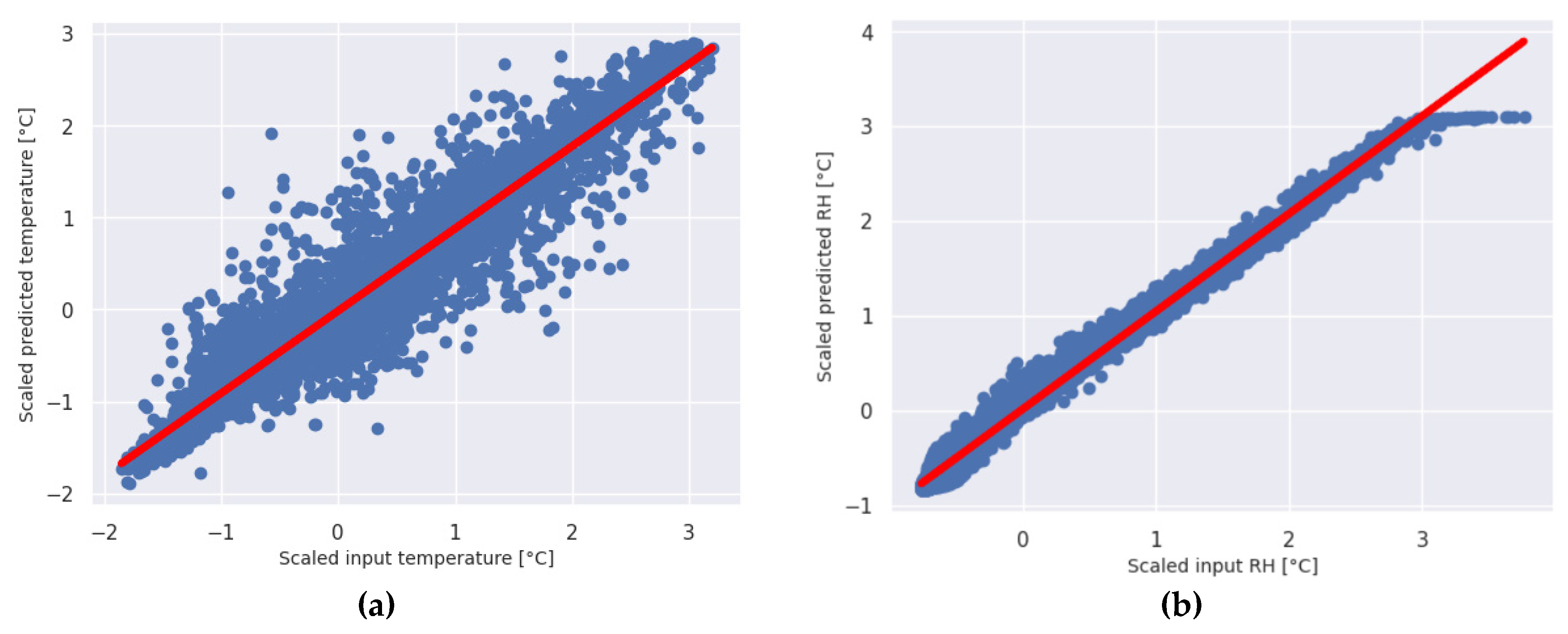
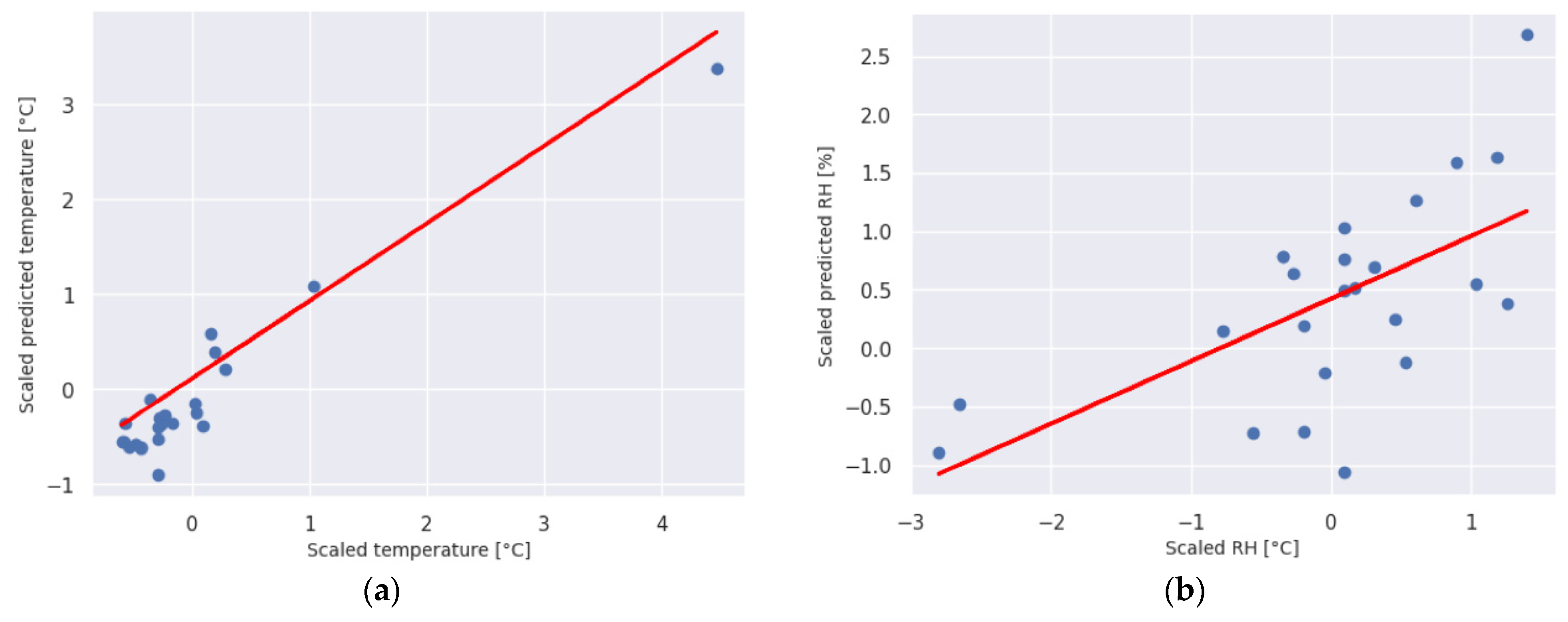
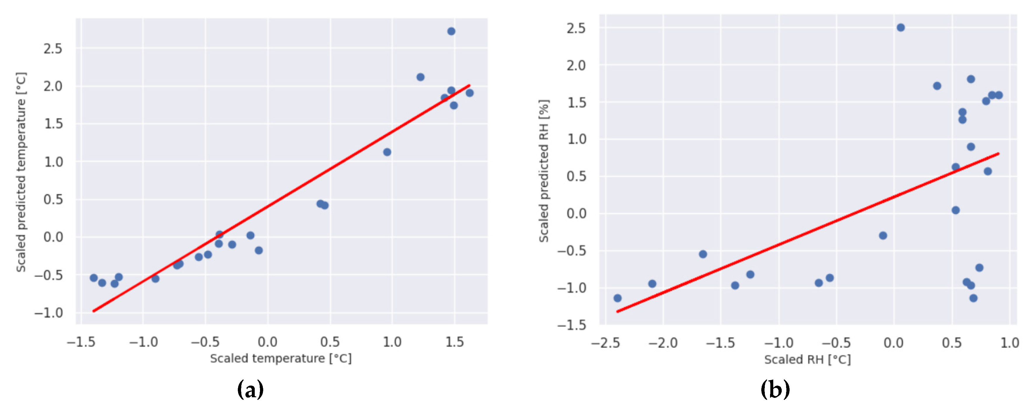
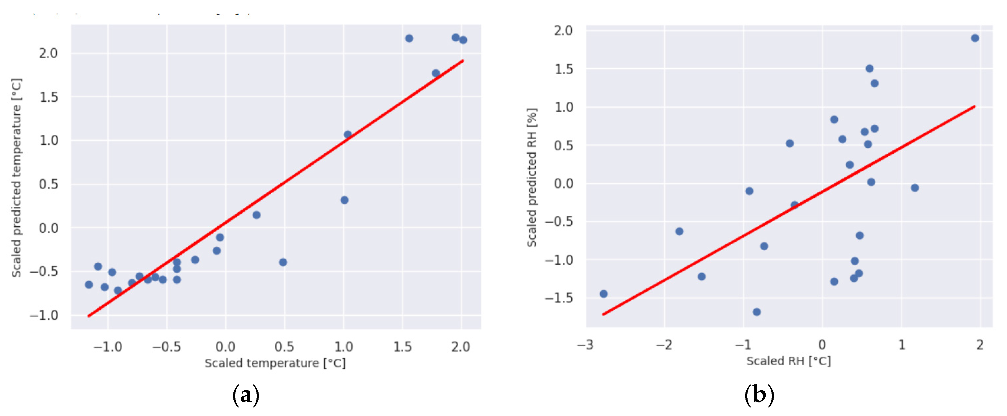
Figure 7 shows the relationship between predicted and TRNSYS data for the train data for mean temperature and relative humidity in the greenhouse, and
Figure 8 shows the relationship between the data for the test data. From the results shown in
Figure 7 and
Figure 8, it can be concluded that the selected model M13 showed a good agreement with the selected data and that it can completely replace the complex TRNSYS model for predicting temperature and relative humidity in the given object. From
Table 3 it can also be seen that the differences in the input data and the data obtained by prediction are very small.
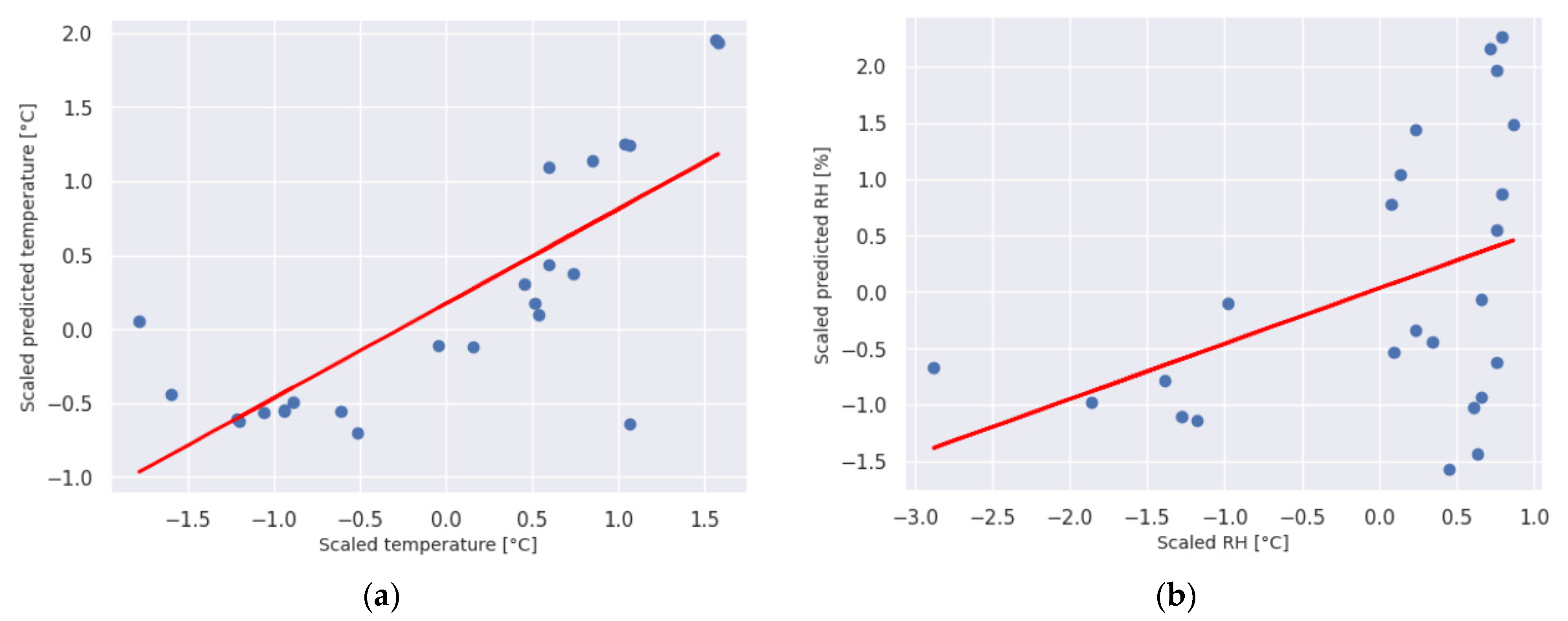
As the TRNSYS model is built using the information about the structure of the object, orientation and all other important inner object features, the predicted values for temperature and relative humidity depend of all parameters within such a complex object. It was stated earlier that the accuracy of the TRNSYS model of the object’s dynamic behavior depends on the accuracy of the data entered in TYPE 56. In the case of the examined greenhouse, the problem is the absence of mechanical ventilation and insufficient natural ventilation, which, together with a system of dewing, significantly affects the relative humidity inside the greenhouse. In order to further check the model, 4 days in the heating season (from 4.11. until 4.12.2022.) with weaker ventilation were chosen. Weaker ventilation was caused by external conditions, high wind speed and the opening of the domes were chosen. The results of the validation of the model with the actual measured data in those days are given respectively in
Figure 9,
Figure 10,
Figure 11 and
Figure 12.
Table 3.
The differences between the input data and the data obtained by prediction.
Table 3.
The differences between the input data and the data obtained by prediction.
| Data |
Parameter |
Equation |
Adj.R2
|
| train |
Temperature |
y = 0.7708*x + 0.0186 |
0.681 |
| Relative humidity |
y = 1.022*x + 0.0105 |
0.989 |
| test |
Temperature |
y = 0.8961*x – 0.0151 |
0.903 |
| Relative humidity |
y = 1.003*x + 0.00187 |
0.997 |
The value of the temperature in the object is primarily a result of the complex thermal load of the object: conduction through the covering of the object, convection at the external and internal surfaces, as well as solar radiation–transmitted, absorbed by internal surfaces and reflected. The actual measured data showed a relatively good match with respect to the average value of Adj. R2, which was in the interval from 0.681 to 0.989, and thus it is showed that for long-term prediction of the mean temperature in the greenhouses, the data obtained from a typical meteorological year, as well as the data obtained by simulations of the physical load of the object can be successfully used instead of the actual measured ones. Smaller variations related to the relative humidity are the result of deviations in real conditions on given days from the predicted model of natural ventilation. Namely, due to the strong wind, the domes were closed, and the moisture model did not fully correspond to the selected moisture model in the TRNSYS model itself, which resulted in a reduced overall accuracy of the model, but however still with a retained trend of correlation between the data.
5. Conclusions
The present study discusses the application and usefulness of artificial neural network-based modeling approach in predicating the greenhouse mean temperature and relative humidity.
In general, the application of ANN gives the possibility of determining non-linear relationships that exist between microclimatic data in buildings, such as temperature and relative humidity, wind speed and direction, direct and diffuse radiation, but also the orientation and geometry of the building, and especially internal loads. In most similar studies, the ANN model was formed on the basis of measured data in the object. However, another approach was applied in this paper, using data obtained from dynamic simulation of thermal load of the object based on meteorological data from a typical meteorological year. In this case, it is meteorological data combined in the period from 2007 to 2021, which opens up the possibility that the ANN model can be used more successfully in a longer period of time, instead of being based only on one-year data. The accuracy of the ANN model depends, first of all, on the accuracy of the TRNSYS model, and the more it corresponds to the real conditions of the object, the higher the accuracy of the obtained results will be. In the facility that is simulated in operation, due to the lack of a mechanical ventilation system, there is a degree of difference in the prediction of the corresponding data, as shown through the values of relative humidity and especially on selected days, when the actual state of ventilation is completely opposite to the previously defined ventilation in the starting model. A 3-layered neural network is designed and trained with the existing dataset and obtained a relationship between the existing non-linear parameters of micro-climate.
In order to find the optimal ANN model, different models were trained by varying hidden neurons, learning rate and epochs. Earlier preliminary analyzes showed that the Mean Squared Error during the training model decreases up to the number of epochs of 400, and in the case of the given ANN model, the optimal number was 331, while the optimal value of the learning rate was 0.079, with 6 hidden neurons.
RMSE and MAE statistical indicators showed small values that demonstrates the correct behavior of the developed forecasting models. The values of the correlation coefficient demonstrate the good agreement between predicted and measured values between temperature and humidity.
With this study, it can be concluded that with the combination of temperatures and relative humidity of the external environment and the object, an ANN model can be formed, which with more satisfactory accuracy can be used for predicting temperatures inside the object and eventual corrections in the heating and ventilation system. Although the results were not fully consistent with the specific parameters obtained by measurements directly on the object, they are certainly encouraging to extend the presented ANN network with more input data and more complex structures in the future.
Author Contributions
O.EĐ.: methodology, software, validation, formal analysis, visualization, investigation, data curation, resources, writing—original draft, writing—review and editing. M.M.: software, formal analysis, validation, data curation, investigation, writing—review and editing. A.DP.: data curation, writing—original draft. Z.M..: formal analysis, writing—review and editing. A.D. (formal analysis, writing—review and editing. R.M.: data curation, formal analysis, writing—review and editing. All authors have read and agreed to the published version of the manuscript.
Data Availability Statement
Dataset available on request from the authors.
Acknowledgments
In this section, you can acknowledge any support given which is not covered by the author contribution or funding sections. This may include administrative and technical support, or donations in kind (e.g., materials used for experiments).
Conflicts of Interest
The authors declare that the research was conducted in the absence of any commercial or financial relationships that could be construed as a potential conflict of interest.
References
- Al-Helal, I.M.; Abdel-Ghany, A.M. Energy Partition and Conversion of Solar and Thermal Radiation into Sensible and Latent Heat in a Greenhouse under Arid Conditions. Energy Build. 2011, 43, 1740–1747. [CrossRef]
- Jirka, V.; Kučeravý, V.; Malý, M.; Pech, F.; Pokorný, J. Energy Flow in a Greenhouse Equipped with Glass Raster Lenses. Renew. Energy 1999, 16, 660–664. [CrossRef]
- Aye, L.; Fuller, R.J.; Canal, A. Evaluation of a Heat Pump System for Greenhouse Heating. Int. J. Therm. Sci. 2010, 49, 202–208. [CrossRef]
- Kürklü, A.; Bilgin, S. Cooling of a Polyethylene Tunnel Type Greenhouse by Means of a Rock Bed. Renew. Energy 2004, 29, 2077–2086. [CrossRef]
- Berroug, F.; Lakhal, E.K.; El Omari, M.; Faraji, M.; El Qarnia, H. Numerical Study of Greenhouse Nocturnal Heat Losses. J. Therm. Sci. 2011, 20, 377–384. [CrossRef]
- Petrakis, T.; Kavga, A.; Thomopoulos, V.; Argiriou, A.A. Neural Network Model for Greenhouse Microclimate Predictions. Agric. 2022, 12, 1–17. [CrossRef]
- Shen, Y.; Wei, R.; Xu, L. Energy Consumption Prediction of a Greenhouse and Optimization of Daily Average Temperature. Energies 2018, 11. [CrossRef]
- Mahmood, F.; Govindan, R.; Bermak, A.; Yang, D.; Khadra, C.; Al-Ansari, T. Energy Utilization Assessment of a Semi-Closed Greenhouse Using Data-Driven Model Predictive Control. J. Clean. Prod. 2021, 324, 129172. [CrossRef]
- Tehnika, P. Energetska Optimizacija Sistema Za Korišćenje Geotermalne Energije Za Grejanje Plastenika. 2008, 49–55.
- Ghosal, M.K.; Tiwari, G.N. Mathematical Modeling for Greenhouse Heating by Using Thermal Curtain and Geothermal Energy. Sol. Energy 2004, 76, 603–613. [CrossRef]
- Fidaros, D.K.; Baxevanou, C.A.; Bartzanas, T.; Kittas, C. Numerical Simulation of Thermal Behavior of a Ventilated Arc Greenhouse during a Solar Day. Renew. Energy 2010, 35, 1380–1386. [CrossRef]
- Dayan, J.; Dayan, E.; Strassberg, Y.; Presnov, E. Simulation and Control of Ventilation Rates in Greenhouses. Math. Comput. Simul. 2004, 65, 3–17. [CrossRef]
- Teitel, M.; Tanny, J. Natural Ventilation of Greenhouses: Experiments and Model. Agric. For. Meteorol. 1999, 96, 59–70. [CrossRef]
- Kittas, C.; Karamanis, M.; Katsoulas, N. Air Temperature Regime in a Forced Ventilated Greenhouse with Rose Crop. Energy Build. 2005, 37, 807–812. [CrossRef]
- Molina-Aiz, F.D.; Fatnassi, H.; Boulard, T.; Roy, J.C.; Valera, D.L. Comparison of Finite Element and Finite Volume Methods for Simulation of Natural Ventilation in Greenhouses. Comput. Electron. Agric. 2010, 72, 69–86. [CrossRef]
- Boulard, T.; Fatnassi, H.; Roy, J.C.; Lagier, J.; Fargues, J.; Smits, N.; Rougier, M.; Jeannequin, B. Effect of Greenhouse Ventilation on Humidity of inside Air and in Leaf Boundary-Layer. Agric. For. Meteorol. 2004, 125, 225–239. [CrossRef]
- Parra, J.P.; Baeza, E.; Montero, J.I.; Bailey, B.J. Natural Ventilation of Parral Greenhouses. Biosyst. Eng. 2004, 87, 355–366. [CrossRef]
- Braun, J.E.; Mitchell, J.C. Solar Geometry for Fixed and Tracking Surfaces. Sol. Energy 1983, 31, 439–444. [CrossRef]
- Zhu, S.; Deltour, J.; Wang, S. Modeling the Thermal Characteristics of Greenhouse Pond Systems. Aquac. Eng. 1998, 18, 201–217. [CrossRef]
- Lim, A. A Comparative Study between TRNSYS and RC Thermal Models to Simulate a District Thermal Demand, 2020.
- Zhang, G.; Ding, X.; Li, T.; Pu, W.; Lou, W.; Hou, J. Dynamic Energy Balance Model of a Glass Greenhouse: An Experimental Validation and Solar Energy Analysis. Energy 2020, 198. [CrossRef]
- Baglivo, C.; Mazzeo, D.; Panico, S.; Bonuso, S.; Matera, N.; Congedo, P.M.; Oliveti, G. Data from a Dynamic Simulation in a Free-Floating and Continuous Regime of a Solar Greenhouse Modelled in TRNSYS 17 Considering Simultaneously Different Thermal Phenomena. Data Br. 2020, 33, 106339. [CrossRef]
- Baglivo, C.; Mazzeo, D.; Panico, S.; Bonuso, S.; Matera, N.; Congedo, P.M.; Oliveti, G. Complete Greenhouse Dynamic Simulation Tool to Assess the Crop Thermal Well-Being and Energy Needs. Appl. Therm. Eng. 2020, 179, 115698. [CrossRef]
- He, F.; Ma, C. Modeling Greenhouse Air Humidity by Means of Artificial Neural Network and Principal Component Analysis. Comput. Electron. Agric. 2010, 71. [CrossRef]
- Taki, M.; Ajabshirchi, Y.; Ranjbar, S.F.; Rohani, A.; Matloobi, M. Heat Transfer and MLP Neural Network Models to Predict inside Environment Variables and Energy Lost in a Semi-Solar Greenhouse. Energy Build. 2016, 110, 314–329. [CrossRef]
- Koirala, A.; Walsh, K.B.; Wang, Z.; McCarthy, C. Deep Learning–Method Overview and Review of Use for Fruit Detection and Yield Estimation. Comput. Electron. Agric. 2019, 162, 219–234. [CrossRef]
- Saleem, M.H.; Potgieter, J.; Arif, K.M. Plant Disease Detection and Classification by Deep Learning. Plants 2019, 8, 32–34. [CrossRef]
- Zhang, Q.; Liu, Y.; Gong, C.; Chen, Y.; Yu, H. Applications of Deep Learning for Dense Scenes Analysis in Agriculture: A Review. Sensors (Switzerland) 2020, 20, 1–33. [CrossRef]
- Pahlavan, R.; Omid, M.; Akram, A. Energy Input-Output Analysis and Application of Artificial Neural Networks for Predicting Greenhouse Basil Production. Energy 2012, 37, 171–176. [CrossRef]
- Uchida Frausto, H.; Pieters, J.G. Modelling Greenhouse Temperature Using System Identification by Means of Neural Networks. Neurocomputing 2004, 56, 423–428. [CrossRef]
- Fandel, G.; Letmathe, P.; Spengler, T.S.; Walther, G. Sustainable Operations. J. Bus. Econ. 2021, 91, 123–125. [CrossRef]
- Singh, V.K.; Tiwari, K.N. Prediction of Greenhouse Micro-Climate Using Artificial Neural Network. Appl. Ecol. Environ. Res. 2017, 15, 767–778. [CrossRef]
- Castañeda-Miranda, A.; Castaño, V.M. Smart Frost Control in Greenhouses by Neural Networks Models. Comput. Electron. Agric. 2017, 137, 102–114. [CrossRef]
- McDowell, T.P.; Emmerich, S.; Thornton, J.W.; Walton, G. Integration of Airflow and Energy Simulation Using CONTAM and TRNSYS. ASHRAE Trans. 2003, 109 PART 2, 757–770.
- Castellucci, S.; Carlini, M. Modelling and Simulation for Energy Production Parametric Dependence in Greenhouses. Math. Probl. Eng. 2010, 2010. [CrossRef]
- SCL Trnsys 18. Sol. Energy Lab. Univ. Wisconsin-Madison 2018, 3, 7–36.
- Djuric, O.E. Non-Isothermal Cavity Mixed Convection Research for Computational Fluid Dynamics and Thermal Behaviour Interoperability Development, University of Belgrade, 2008.
- Kanzow, C.; Yamashita, N.; Fukushima, M. Levenberg-Marquardt Methods with Strong Local Convergence Properties for Solving Nonlinear Equations with Convex Constraints. J. Comput. Appl. Math. 2004, 172, 375–397. [CrossRef]
- Kim, S.Y.; Lee, S.M.; Park, K.S.; Ryu, K.H. Prediction Model of Internal Temperature Using Backpropagation Algorithm for Climate Control in Greenhouse. Hortic. Sci. Technol. 2018, 36, 713–729. [CrossRef]
|
Disclaimer/Publisher’s Note: The statements, opinions and data contained in all publications are solely those of the individual author(s) and contributor(s) and not of MDPI and/or the editor(s). MDPI and/or the editor(s) disclaim responsibility for any injury to people or property resulting from any ideas, methods, instructions or products referred to in the content. |
© 2024 by the authors. Licensee MDPI, Basel, Switzerland. This article is an open access article distributed under the terms and conditions of the Creative Commons Attribution (CC BY) license (http://creativecommons.org/licenses/by/4.0/).


