Review of Fourth-Order Maximum Entropy Based Predictive Modelling and Illustrative Application to a Nuclear Reactor Benchmark. I. Typical High-Order Sensitivity and Uncertainty Analysis

Preprint

Review

Review of Fourth-Order Maximum Entropy Based Predictive Modelling and Illustrative Application to a Nuclear Reactor Benchmark. I. Typical High-Order Sensitivity and Uncertainty Analysis

Altmetrics

Downloads

Views

Comments

A peer-reviewed article of this preprint also exists.

This version is not peer-reviewed

Submitted:

25 March 2024

Posted:

25 March 2024

You are already at the latest version

Alerts

Abstract

This work (in two parts) will review the recently developed predictive modeling methodology called “4th-BERRU-PM” and its applicability to energy systems as exemplified by an illustrative application to the Polyethylene-Reflected Plutonium (acronym: PERP) OECD/NEA reactor physics benchmark. The acronym 4th-BERRU-PM designates the “Fourth-Order Best-Estimate Results with Reduced Uncertainties Predictive Modeling” methodology, which yields best-estimate results with reduced uncertainties for the first fourth-order moments (mean values, covariance, skewness, and kurtosis) of the optimally predicted posterior distribution of model results and calibrated model parameters. The 4th-BERRU-PM uses the Maximum Entropy (MaxEnt) principle to incorporate fourth-order experimental and computational information, including fourth (and higher) order sensitivities of computed model responses to model parameters, thus incorporating, as particular cases, the results previously predicted by the second-order predictive modeling methodology 2nd-BERRU-PM, and vastly generalizing the results produced by extant data assimilation and data adjustment procedures. The 4th-BERRU-PM methodology encompasses the scopes of high-order sensitivity analysis (SA), uncertainty quantification (UQ), data assimilation (DA) and model calibration (MC). The application of the 4th-BERRU-PM methodology to energy systems is illustrated by means of the above-mentioned OECD/NEA reactor physics benchmark, which is modeled using the neutron transport Boltzmann equation involving 21976 imprecisely known parameters, the solution of which is representative of “large-scale computations.” The model result (“response”) of interest is the leakage of neutrons through the outer surface of this spherical benchmark, which can be computed numerically and measured experimentally. Part 1 of this work illustrates the impact of high-order sensitivities, in conjunction with parameter standard deviations of various magnitudes, on the determination of the expected value and variance of the computed response in terms of the first four moments of the distribution of the uncertain model parameters. Part 2 of this work will illustrate the capabilities of the 4th-BERRU-PM methodology for combining computational and experimental information, up to and including forth-order sensitivities and distributional moments, for producing best-estimate values for the predicted responses and model parameters while reducing their accompanying uncertainties.

Keywords:

Subject: Physical Sciences - Applied Physics

1. Introduction

This work briefly reviews the “4^th-Order Best-Estimate Results with Reduced Uncertainties Predictive Modeling” (abbreviated as “4^th-BERRU-PM”) methodology developed recently by Cacuci [1] and illustrates its application to energy systems by considering the Polyethylene-Reflected Plutonium (acronym: PERP) OECD/NEA reactor physics benchmark [2]. The 4^th-BERRU-PM uses the Maximum Entropy (MaxEnt) Principle [3] to combine sensitivities and moments (up to and including fourth-order) of the distribution of model parameters and model responses (i.e., results of interest) which stem from model computations and imprecisely known external experimental measurements. Using this high-order computational and experimental information, the 4^th-BERRU-PM methodology yields the 4^th-order MaxEnt joint posterior distribution of model parameters and responses. In particular, this posterior distribution yields best-estimate results for the optimally predicted moments (up to and including fourth-order) of the best-estimate predicted model parameters (“model calibration”) and predicted responses. The 4^th-BERRU-PM methodology encompasses the scopes of high-order sensitivity analysis (SA), uncertainty quantification (UQ), data assimilation (DA) and model calibration (MC). The 4^th-BERRU-PM methodology is currently peerless and includes, as particular cases, the results delivered by the second-order “2^nd-BERRU-PM” predictive modeling methodology developed by Cacuci [4,5], while vastly generalizing the extant data adjustment [6,7] and data assimilation methodologies [8,9,10,11,12].

The fundamental importance of the new results provided by the 4^th-BERRU-PM methodology will be highlighted in this work by applying this predictive modeling methodology to the Polyethylene-Reflected Plutonium OECD/NEA reactor physics benchmark [2]. As has been detailed by Cacuci and Fang [13], the numerical modeling of the PERP benchmark is performed by using the neutron transport Boltzmann equation, involving 21976 imprecisely known parameters. The response (i.e., result) of interest for this benchmark is the total leakage of neutrons through the benchmark’s outer surface. The computation of high-order sensitivities of the leakage response with respect to the benchmark’s parameters is representative of “large-scale computations” and has been accomplished by applying the high-order adjoint sensitivity analysis methodology developed by Cacuci [14,15], which overcomes the curse of dimensionality [16] in sensitivity analysis.

Section 2 of this work reviews the mathematical forms of the “input information” that needs to be extracted from the computational model to be incorporated into the 4^th-BERRU-PM methodology. Extracting this information requires performing a “4^th-order sensitivity analysis” (4^th-SA) and a “4^th-order uncertainty quantification” (4^th-UQ) of the computational model by propagating the first four moments (including the means, variances, skewness, kurtosis) of the distribution of model parameters using the response sensitivities (from first- to fourth-order) to obtain the requisite moments (from first to fourth) of the distribution of computed responses. This Section also discusses briefly the computational issues required to alleviate the impact of the ”curse of dimensionality” [16]) when computing such 4^th-order sensitivities and uncertainties for energy systems.

Section 3 presents the application of the mathematical concepts reviewed in Section 2 to the PERP reactor physics benchmark, illustrating the effect of the high-order sensitivities on the expected value and variance of the computed model response, when considering: (i) parameters that are known with “high precision” having uniform standard deviations of 2%; (ii) parameters known with “medium precision” having uniform standard deviations of 5%; and (iii) parameters known with “low precision” having uniform standard deviations of 10%, respectively. Section 4 concludes this work by discussing the impact of the combination of parameter uncertainties with high-order sensitivities on the uncertainties in the computed model, and also prepares the ground for the continuation, in the accompanying Part 2 [17], of the application of the 4^th-BERRU-PM methodology for obtaining predicted best-estimate mean value, standard deviation, skewness, and kurtosis for the neutron leakage response of the PERP benchmark.

2. Model Sensitivity and Uncertainty Analysis Input for the Fourth-Order Maximum Entropy Based Predictive Modeling Methodology (4th-BERRU-PM): Review and Applicability to Energy Systems

The 4^th-BERRU-PM methodology uses as “input” the first four moments of the unknown distributions of the responses computed using a mathematical/computational model, which are combined using the maximum entropy principle with the first four moments of the distribution of measured responses. The moments of the distribution of the computed model responses are obtained by combining the moments of the distribution of model parameters with the sensitivities of the model responses with respect to the model parameters. Thus, the moments of the distribution of the computed model responses are obtained by performing (simultaneously or sequentially) a 4^th-order sensitivity analysis and a 4^th-order uncertainty analysis of the underlying mathematical/computational model.

The mathematical expressions of the moments of the computed responses are obtained in terms of the moments of the distribution of model parameters by expanding formally each response in a Taylor-series around the nominal or mean parameter values and subsequently using this series, within its radius of convergence, for obtaining expressions of the moments of the respective responses in terms of the moments of the model parameters and the response sensitivities (i.e., derivatives) with respect to the model parameters. General expressions, up to sixth-order sensitivities, for the moments of computed responses can be found in the book by Cacuci [14], which generalizes the expressions originally obtained by Tukey [18]. In particular, the following fourth-order Taylor-series expansion of a response, denoted as

r_{k} (α)

, as a function of the parameters

α ≜ {(α_{1}, \dots, α_{T P})}^{†}

, where

T P

denotes the total number of parameters under consideration, is used within the 4^th-BERRU-PM methodology to compute the various moments of the distribution of the leakage response in the phase-space of the benchmark’s total cross section (parameters):

\begin{array}{l} r_{k} (α) = r_{k} (α^{0}) + \sum_{j_{1} = 1}^{T P} {\frac{\partial r_{k} (α)}{\partial α_{j_{1}}}}_{α^{0}} δ t_{j_{1}} + \frac{1}{2} \sum_{j_{1} = 1}^{T P} \sum_{j_{2} = 1}^{T P} {\frac{\partial^{2} r_{k} (α)}{\partial α_{j_{1}} \partial α_{j_{2}}}}_{α^{0}} δ α_{j_{1}} δ α_{j_{2}} \\ + \frac{1}{3!} \sum_{j_{1} = 1}^{T P} \sum_{j_{2} = 1}^{T P} \sum_{j_{3} = 1}^{T P} {\frac{\partial^{3} r_{k} (α)}{\partial α_{j_{1}} \partial α_{j_{2}} \partial α_{j_{3}}}}_{α^{0}} δ α_{j_{1}} δ α_{j_{2}} δ α_{j_{3}} \\ + \frac{1}{4!} \sum_{j_{1} = 1}^{T P} \sum_{j_{2} = 1}^{T P} \sum_{j_{3} = 1}^{T P} \sum_{j_{4} = 1}^{T P} {\frac{\partial^{4} r_{k} (α)}{\partial α_{j_{1}} \partial α_{j_{2}} \partial α_{j_{3}} \partial α_{j_{4}}}}_{α^{0}} δ α_{j_{1}} δ α_{j_{2}} δ α_{j_{3}} δ α_{j_{4}} + ε_{k} . \end{array}

(1)

In Eq. (1), the notation

{}_{α^{0}}

indicates that the functional derivatives within the braces are computed at the known expected/nominal parameter values, which are denoted as

α_{i}^{0}

(using the superscript “0”); the corresponding column vector of nominal parameter values is denoted as

α^{0} ≜ {(α_{1}^{0}, \dots, α_{T P}^{0})}^{†}

. The quantity

ε_{k}

comprises all quantifiable errors in the representation of the computed response

r_{k} (α)

as a function of the model parameters

α ≜ {(α_{1}, \dots, α_{T P})}^{†}

. Vector and matrices will be denoted using bold letters while the dagger “

†

” will be used to denote “transposition.” The symbol “

≜

” will be used to denote “is defined as” or “is by definition equal to.” The radius/domain of convergence of the series in Eq. (1) determines the largest values of the parameter variations

δ α_{j}

which are admissible before the respective series becomes divergent. In turn, these maximum admissible parameter variations limit the largest parameter covariances/standard deviations which are acceptable for using the Taylor-expansion for computing moments of the distribution of computed responses.

2.1. Input to 4^th-BERRU-PM Methodology: 4th-Order Sensitivity and Uncertainty Analysis of Model Responses to Model Parameters

The moments of the computed model responses are obtained by using the Taylor-series expansion shown in Eq. (1) of a response in terms of parameter variations. The expression of these computed response moments up to sixth-order in moments and the parameter distribution and sensitivities can be found in the book by Cacuci [14]. The 4^th-BERRU-PM methodology incorporates computed response moments up to fourth-order, as provided below.

(i): The expected value, denoted as $E_{c} (r_{k})$ , of a computed response $r_{k} (α)$ , for $k = 1, \dots, T R$ ; the vector $E_{c} (r)$ of the computed responses is defined as follows: $E_{c} (r) ≜ {[E_{c} (r_{1}), \dots, E_{c} (r_{k}), \dots, E_{c} (r_{T R})]}^{†}$ . Up to, and including, the fourth-order response sensitivities to parameters, the expected value of a computed response has the following expression obtained by integrating formally Eq. (1) over the unknown distribution of parameters:

$\begin{array}{l} E_{c} (r_{k}) = r_{k} (α^{0}) + \frac{1}{2} \sum_{i = 1}^{T P} \sum_{j = 1}^{T P} {\frac{\partial^{2} r_{k} (α)}{\partial α_{i} \partial α_{j}}}_{α^{0}} c_{i j}^{α} + \frac{1}{6} \sum_{i = 1}^{T P} \sum_{j = 1}^{T P} \sum_{ℓ = 1}^{T P} {\frac{\partial^{3} r_{k} (α)}{\partial α_{i} \partial α_{j} \partial α_{ℓ}}}_{α^{0}} t_{i j ℓ}^{α} \\ + \frac{1}{4!} \sum_{i = 1}^{T P} \sum_{j = 1}^{T P} \sum_{ℓ = 1}^{T P} \sum_{m = 1}^{T P} {\frac{\partial^{4} r_{k} (α)}{\partial α_{i} \partial α_{j} \partial α_{ℓ} \partial α_{m}}}_{α^{0}} q_{i j ℓ m}^{α} + \dots \end{array}$

(2)

In Eq. (2), the moments up to and including fourth-order of the unknown distribution of model parameters are assumed to be known. These moments are as follows: (a) the covariances of two model parameters, $α_{i}$ and $α_{j}$ , are denoted as $c_{i j}^{α}$ , $i, j = 1, \dots, T P$ , where $T P$ denotes the total number of parameters under consideration; the parameter covariance matrix is denoted as $C_{α α} ≜ {[c_{i j}^{α}]}_{T P \times T P}$ ; (b) the triple-correlations of three model parameters $α_{i}$ , $α_{j}$ , and $α_{l}$ , are denoted as $t_{i j ℓ}^{α}$ , where $i, j, ℓ = 1, \dots, T P$ ; (c) the quadruple-correlations of four model parameters $α_{i}$ , $α_{j}$ , $α_{ℓ}$ , and $α_{m}$ , are denoted as $q_{i j ℓ m}^{α}$ , where $i, j, ℓ, m = 1, \dots, T P$ .
(ii): The correlation, denoted as $cor (α_{i}, r_{k})$ , between a parameter $α_{i}$ and a computed response $r_{k}$ , for $i = 1, \dots, T P$ and $k = 1, \dots, T R$ ; the correlation matrix between parameters and computed responses is denoted as $C_{α r}^{c} ≜ {[cor (α_{i}, r_{k})]}_{T P \times T R}$ . Up to, and including, the fourth-order response sensitivities to parameters, the correlation between a parameter and a computed response has the following expression:

$\begin{array}{l} cor (α_{i}, r_{k}) = \sum_{j = 1}^{T P} {\frac{\partial r_{k} (α)}{\partial α_{j}}}_{α^{0}} c_{i j}^{α} + \frac{1}{2} \sum_{j = 1}^{T P} \sum_{ℓ = 1}^{T P} {\frac{\partial^{2} r_{k} (α)}{\partial α_{j} \partial α_{ℓ}}}_{α^{0}} t_{i j ℓ}^{α} \\ + \frac{1}{6} \sum_{j = 1}^{T P} \sum_{ℓ = 1}^{T P} \sum_{m = 1}^{T P} {\frac{\partial^{3} r_{k} (α)}{\partial α_{j} \partial α_{ℓ} \partial α_{m}}}_{α^{0}} q_{i j ℓ m}^{α} + \dots \end{array}$

(3)
(iii): The covariances, denoted as $cov (r_{k}, r_{ℓ})$ , between two computed responses $r_{k}$ and $r_{ℓ}$ , for $k, ℓ = 1, \dots, T R$ ; the covariance matrix of computed responses is denoted as $C_{r r}^{c} ≜ {[cov (r_{k}, r_{ℓ})]}_{T R \times T R}$ . Up to and including the fourth-order response sensitivities to parameters, the covariance between two computed responses has the following expression:

$\begin{array}{l} cov (r_{k}, r_{ℓ}) = \sum_{i = 1}^{T P} \sum_{j = 1}^{T P} {\frac{\partial r_{k} (α)}{\partial α_{i}} \frac{\partial r_{ℓ} (α)}{\partial α_{j}}}_{α^{0}} c_{i j}^{α} \\ + \frac{1}{2} \sum_{i = 1}^{T P} \sum_{j = 1}^{T P} \sum_{m = 1}^{T P} {\frac{\partial^{2} r_{k} (α)}{\partial α_{i} \partial α_{j}} \frac{\partial r_{ℓ} (α)}{\partial α_{m}} + \frac{\partial r_{k} (α)}{\partial α_{i}} \frac{\partial^{2} r_{ℓ} (α)}{\partial α_{j} \partial α_{m}}}_{α^{0}} t_{i j m}^{α} \\ + \frac{1}{4} \sum_{i = 1}^{T P} \sum_{j = 1}^{T P} \sum_{m = 1}^{T P} \sum_{n = 1}^{T P} {\frac{\partial^{2} r_{k} (α)}{\partial α_{i} \partial α_{j}} \frac{\partial^{2} r_{ℓ} (α)}{\partial α_{m} \partial α_{n}}}_{α^{0}} (q_{i j m n}^{α} - c_{i j}^{α} c_{m n}^{α}) \\ + \frac{1}{6} \sum_{i = 1}^{T P} \sum_{j = 1}^{T P} \sum_{m = 1}^{T P} \sum_{n = 1}^{T P} {\frac{\partial^{3} r_{k} (α)}{\partial α_{i} \partial α_{j} \partial α_{m}} \frac{\partial r_{ℓ} (α)}{\partial α_{n}} + \frac{\partial r_{k} (α)}{\partial α_{i}} \frac{\partial^{3} r_{ℓ} (α)}{\partial α_{j} \partial α_{m} \partial α_{n}}}_{α^{0}} q_{i j m n}^{α} + \dots \end{array}$

(4)
(iv): The triple correlations among three responses, $r_{k}$ , $r_{ℓ}$ and $r_{m}$ , $k, ℓ, m = 1, \dots, T R$ , which are denoted as $μ_{3} (r_{k}, r_{ℓ}, r_{m})$ . Up to and including the fourth-order response sensitivities to parameters, these triple correlations among three responses have the following expression:

$\begin{array}{l} μ_{3} (r_{k}, r_{ℓ}, r_{m}) = \sum_{i = 1}^{T P} \sum_{j = 1}^{T P} \sum_{μ = 1}^{T P} {\frac{\partial r_{k} (α)}{\partial α_{i}} \frac{\partial r_{ℓ} (α)}{\partial α_{j}} \frac{\partial r_{m} (α)}{\partial α_{μ}}}_{α^{0}} t_{i j μ}^{α} \\ + \frac{1}{2} \sum_{i = 1}^{T P} \sum_{j = 1}^{T P} \sum_{μ = 1}^{T P} \sum_{ν = 1}^{T P} {\frac{\partial r_{k} (α)}{\partial α_{i}} \frac{\partial r_{ℓ} (α)}{\partial α_{j}} \frac{\partial^{2} r_{m} (α)}{\partial α_{μ} \partial α_{ν}} (q_{i j μ ν}^{α} - c_{i j}^{α} c_{μ ν}^{α}) \\ + {\frac{\partial r_{k} (α)}{\partial α_{i}} \frac{\partial^{2} r_{ℓ} (α)}{\partial α_{j} \partial α_{μ}} \frac{\partial r_{m} (α)}{\partial α_{ν}} (q_{i j μ ν}^{α} - c_{i ν}^{α} c_{j μ}^{α})}}_{α^{0}} + \dots \end{array}$

(5)
(v): The quadruple-correlations among four responses, $r_{k}$ , $r_{ℓ}$ , $r_{m}$ and $r_{n}$ , for $k, ℓ, m, n = 1, \dots, T R$ , which are denoted as $μ_{4} (r_{k}, r_{ℓ}, r_{m}, r_{n})$ . Up to and including the fourth-order response sensitivities to parameters, these quadruple correlations among computed responses have the following expression:

$μ_{4} (r_{k}, r_{ℓ}, r_{m}, r_{n}) = \sum_{i = 1}^{T P} \sum_{j = 1}^{T P} \sum_{μ = 1}^{T P} \sum_{ν = 1}^{T P} {\frac{\partial r_{k} (α)}{\partial α_{i}} \frac{\partial r_{l} (α)}{\partial α_{j}} \frac{\partial r_{m} (α)}{\partial α_{μ}} \frac{\partial r_{n} (α)}{\partial α_{ν}}}_{α^{0}} q_{i j μ ν}^{α} + \dots$

(6)
(vi): The expressions of the triple and quadruple correlations among parameters and responses are provided by Cacuci [14]; they will not be reproduced here because they are considered to be negligible by comparison to the other terms used within the 4^th-BERRU-PM methodology.

2.2. Applicability of the 4th-Order Sensitivity and Uncertainty Analysis to Energy Systems

The expressions of the moments of the distribution of computed responses provided in Eqs. (2)‒(6) involve combinations of sensitivities of responses with respect to model parameters and moments of the distribution of parameters. Consequently, the computation of these moments is tantamount to performing both a “4^th-order sensitivity analysis” (since one needs to compute the respective sensitivities) as well as a “4^th-order uncertainty analysis” (since one determines the respective moments of the distribution of the computed response in the phase-space of the model’s parameters) of the computational model under consideration. In principle, sensitivity and uncertainty analyses can be performed by using either deterministic or statistical methods. The statistical methods construct an approximate response distribution (often called “response surface”) in the parameters’ space by performing many “forward” computations using the model with altered parameter values, and subsequently use scatter plots, regression, rank transformation, correlations, and/or so-called “partial correlation analysis” in order to identify approximate expectation values, variances and covariances for the responses. These statistical quantities are subsequently used to construct quantities that play the role of (approximate) first-order response sensitivities. Thus, statistical methods commence with “uncertainty analysis” and subsequently attempt an approximate “sensitivity analysis” of the approximately computed model “response surface”. Statistical methods for uncertainty and sensitivity analysis are reviewed in the book edited by Saltarelli et al. [19]. Although statistical methods for uncertainty and sensitivity analysis are conceptually easy to implement, they are subject to the curse of dimensionality [16] and cannot compute any sensitivity exactly. Also, since the response sensitivities and parameter uncertainties are inseparably amalgamated within the results produced by statistical methods, improvements in parameter uncertainties cannot be directly propagated to improve response uncertainties; rather, the entire set of simulations and statistical post-processing must be repeated anew. On the other hand, the computation by conventional deterministic methods of the

n^{t h}

-order sensitivities (i.e., functional derivatives of a response with respect to the

T P

-parameters on which it depends) would also require at least

O (T P^{n})

large-scale computations, so these methods also suffer from the curse of dimensionality in sensitivity analysis.

Currently, the only methodologies that enable the exact and efficient computation of arbitrarily high-order sensitivities while overcoming the curse of dimensionality are the “n^th-order Comprehensive Adjoint Sensitivity Analysis Methodology for Response-Coupled Forward/Adjoint Linear Systems” (n^th-CASAM-L) conceived by Cacuci [14] and the “n^th-order Comprehensive Adjoint Sensitivity Analysis Methodology for Nonlinear Systems” (n^th-CASAM-N) conceived by Cacuci [15]. These methods are applicable to compute exactly and efficiently arbitrarily-high order sensitivities of responses with respect to parameters for mathematical/computational models of any energy system. The higher the order of computed sensitivities, the higher the efficiency of the n^th-CASAM-L or n^th-CASAM-N methodologies by comparison to any other method. For example, as has been illustrated by Cacuci and Fang [13] and as will be discussed in Section 3, below, the most important sensitivities of the PERP leakage response are with respect to the 180 uncertain total microscopic cross sections. For these sensitivities, the n^th-CASAM-L needs a single “large-scale” adjoint computation to obtain all of the 180 first-order sensitivities exactly, by comparison to needing 360 large-scale computations to obtain them inexactly, using finite differences. Similarly, the n^th-CASAM-L needs 2,075,341 large-scale computations to obtain the 45,212,895 distinct 4^th-order sensitivities exactly, while using finite differences would require 723,404,160 large-scale computations to obtain them approximately.

3. Illustrative High-Order Uncertainty Analysis of the PERP Reactor Physics Benchmark

The Polyethylene-Reflected Plutonium (acronym: PERP) reactor physics benchmark [2] is a one-dimensional spherical subcritical nuclear system driven by a source of spontaneous fission neutrons. The computational model of the polyethylene PERP benchmark used in this work is the same as has been presented by Cacuci and Fang [13]. For convenience, the main features of this model are summarized in the Appendix. As discussed in the Appendix, this benchmark comprises 21976 imprecisely known model parameters. The result (“response”) of interest for this benchmark is the total leakage of neutrons through the benchmark’s outer surface. Since the correlations between these parameters are unavailable, they will be considered to be uncorrelated and normally distributed, in accordance with the principle of Maximum Entropy of considering the least biased distribution based on the available information. Since the parameters are considered to be uncorrelated, the off-diagonal terms of

C_{α α}

vanish, i.e.,

c_{i j}^{α} = 0

when

i \neq j

, while the diagonal terms are the variances of the respective parameters, denoted as

c_{i}^{α}

, for

i = 1, \dots, T P

. Since the parameters are considered to be normally distributed, their third-order (triple) correlations vanish, i.e.,

t_{i j k}^{α} ≜ c o r (α_{i}, α_{j}, α_{k}) = 0

for all

i, j, k = 1, \dots, T P

. Furthermore, the only nonzero fourth-order (quadruple) correlation is the kurtosis of each individual parameter, which will be denoted as

q_{i}^{α}

i = 1, \dots, T P

, which is related to the variance of the respective uncorrelated parameter as follows:

q_{i}^{α} = 3 c_{i}^{α}

, where

c_{i}^{α}

denotes the variance (i.e., standard deviation squared) of the parameter

α_{i}

; all other quadruple correlations vanish, i.e.,

q_{i j k ℓ}^{α} = 0

i \neq j \neq k \neq ℓ

The comprehensive computation of response sensitivities with respect to the model parameters, up to and including fourth-order sensitivities, was performed by Cacuci and Fang [13], where it was shown that the most important parameters are the 180 group-averaged microscopic total cross sections. As has been discussed in the forgoing, these parameters are considered to be uncorrelated; therefore, only the unmixed sensitivities are influential. The largest unmixed sensitivities occur for isotope 6 (¹H). Table 1, below, presents a comparison of the values of the unmixed relative sensitivities, from first-order through fourth-order, for isotope 6 (¹H). Sensitivities that have absolute values larger than unity are presented in bold characters. As shown in Table 1, the largest absolute values for the 1^st-, 2^nd-, 3^rd- and 4^th-order unmixed relative sensitivities all occur for the lowest-energy group (g = 30; thermal neutrons), which are significantly larger than the values of the sensitivities in other energy groups. Notably, the largest 4^th-order unmixed relative sensitivity attains a very large value:

S^{(4)} (σ_{t, 6}^{g = 30}, σ_{t, 6}^{g = 30}, σ_{t, 6}^{g = 30}, σ_{t, 6}^{g = 30}) = 2.720 \times 10^{6}

. By comparison, the largest values for the 1^st-, 2^nd- and 3^rd-order unmixed relative sensitivities are:

S^{(1)} (σ_{t, 6}^{g = 30}) = - 9.366

S^{(2)} (σ_{t, 6}^{g = 30}, σ_{t, 6}^{g = 30}) = 4.296 \times 10^{2}

and

S^{(3)} (σ_{t, 6}^{g = 30}, σ_{t, 6}^{g = 30}, σ_{t, 6}^{g = 30}) = - 2.966 \times 10^{4}

, respectively.

The effects of various values for the standard deviations for the parameters, which are considered to be uncorrelated and normally distributed, will be illustrated in Subsections 3.1‒3.3, below, for parameters that are known with “high precision” (having uniform standard deviations of 2%); parameters known with “medium precision” (having uniform standard deviations of 5%); and parameters known with “low precision” (having uniform standard deviations of 10%), respectively.

3.1.“High Precision” Parameters, Having Uniform Relative Standard Deviations

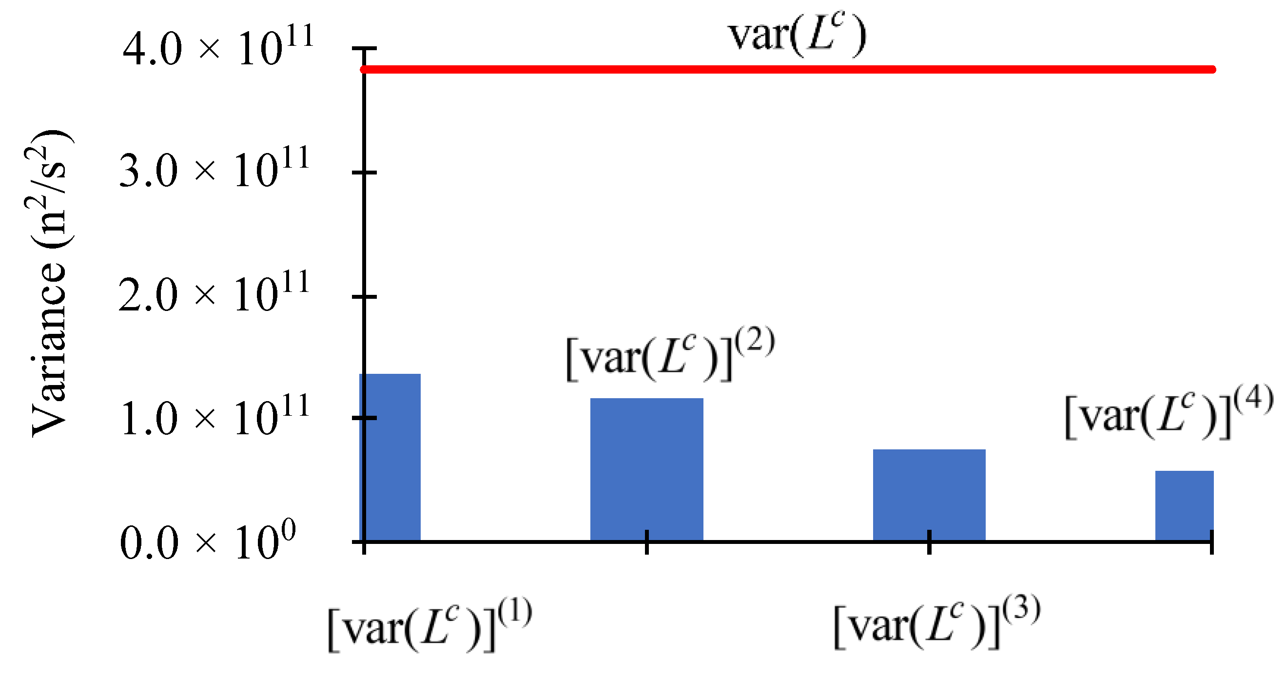
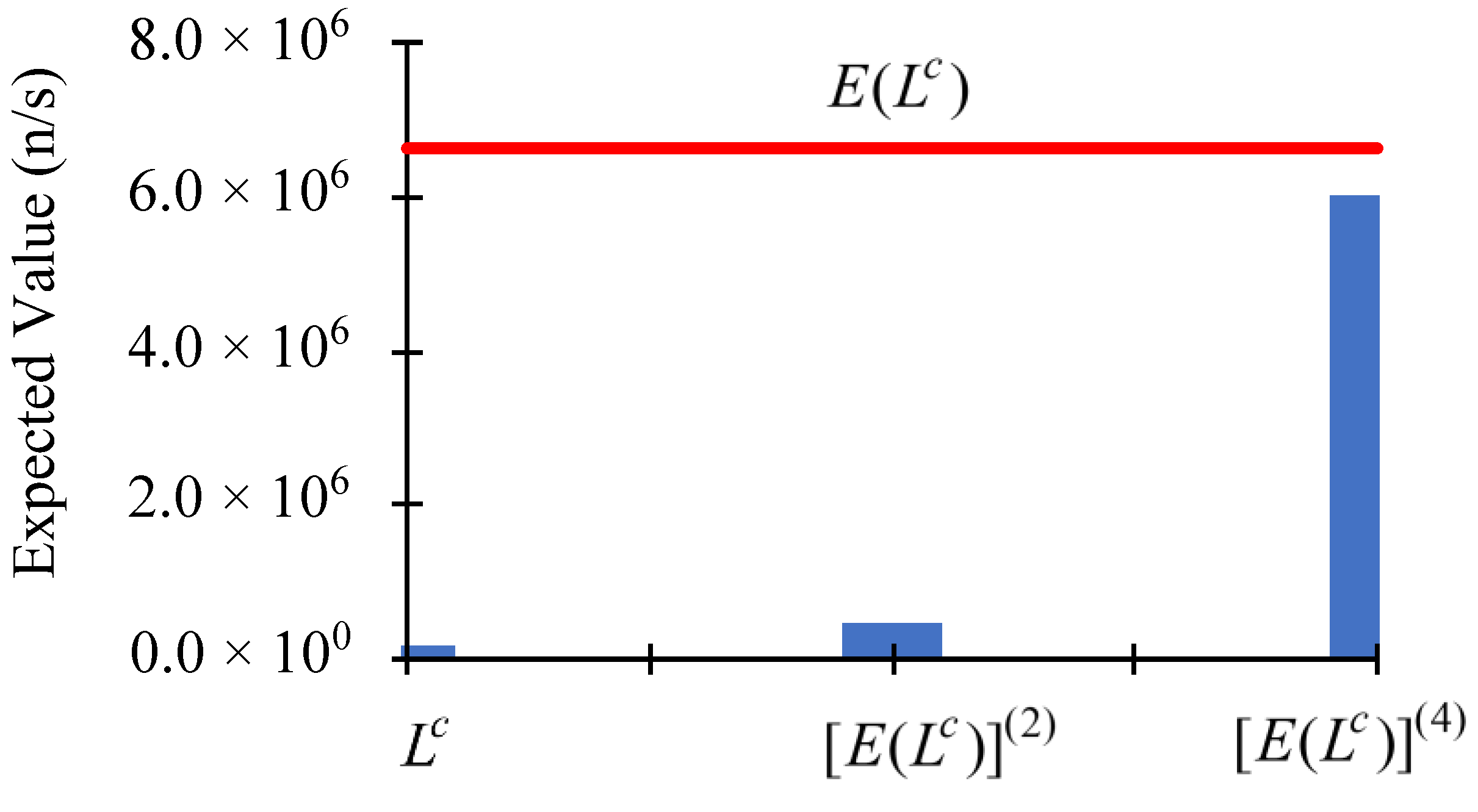
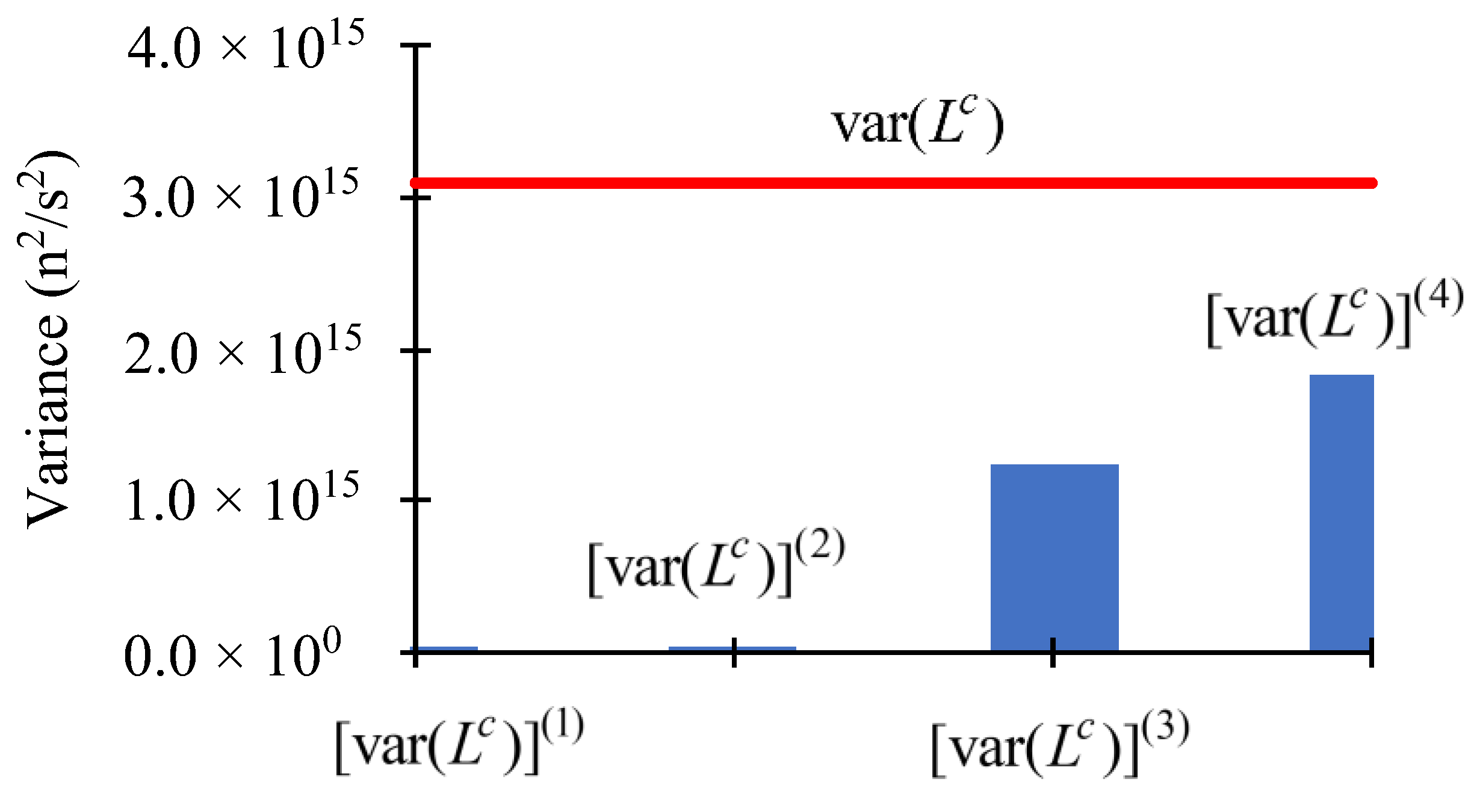
As has been discussed by Cacuci and Fang [13], when the uncorrelated and normally-distributed parameters are assumed to have uniform relative standard deviations of 3%, the convergence “ratio-test” of the 3^rd-order term with respect to the 2^nd-order term of the Taylor series is 0.58, while the ratio of the 4^th-order term with respect to the 3^rd-order term of the Taylor series is 0.68. Both of these results are below 1.00, which implies that for uniform relative standard deviations of 3% or less, the Taylor-series expansion of the computed response in terms of the model parameters shown in Eq. (1) is expected to be convergent. Figure 1 depicts the magnitudes of the higher-order contributions to the expected value,

E (L^{c})

, of the computed leakage response, while Figure 2 depicts the magnitudes of the higher-order contributions to the variance,

var (L^{c})

, of the computed leakage response, for parameters that are assumed to have uniform relative standard deviations of 2% (which is smaller than 3%). The numerical results depicted in Figure 1 and Figure 2 indicate that the contributions of the increasingly higher-order terms to the expected value,

E (L^{c})

, and the variance,

var (L^{c})

, of the computed leakage response become increasingly smaller (as the order of the respective terms increases), thus confirming the expectation that the underlying Taylor-series is convergent. For practical purposes, therefore, the contributions from terms involving sensitivities of order five and higher become negligible by comparison to the contributions from the terms comprising the sensitivities of first-through fourth-order to

E (L^{c})

and

var (L^{c})

, respectively, when the uncorrelated and normally-distributed parameters have uniform relative standard deviations

S D = 2 %

3.2.“Medium Precision” Parameters, Having Uniform Relative Standard Deviations

For uniform relative standard deviations of 5% for the uncorrelated and normally-distributed model parameters, it has been shown by Cacuci and Fang [13] that the ratio of the 3^rd-order term with respect to the 2^nd-order term of the Taylor series is 0.97<1.00, but the ratio of the 4^th-order term with respect to the 3^rd-order term of the Taylor series is 1.13>1.00. These ratios indicate that relative standard deviations of 5% for the model parameters are outside of the radius of convergence of the Taylor-series presented in Eq. (1). These indications are confirmed by the results depicted in Figure 3 and Figure 4, below.

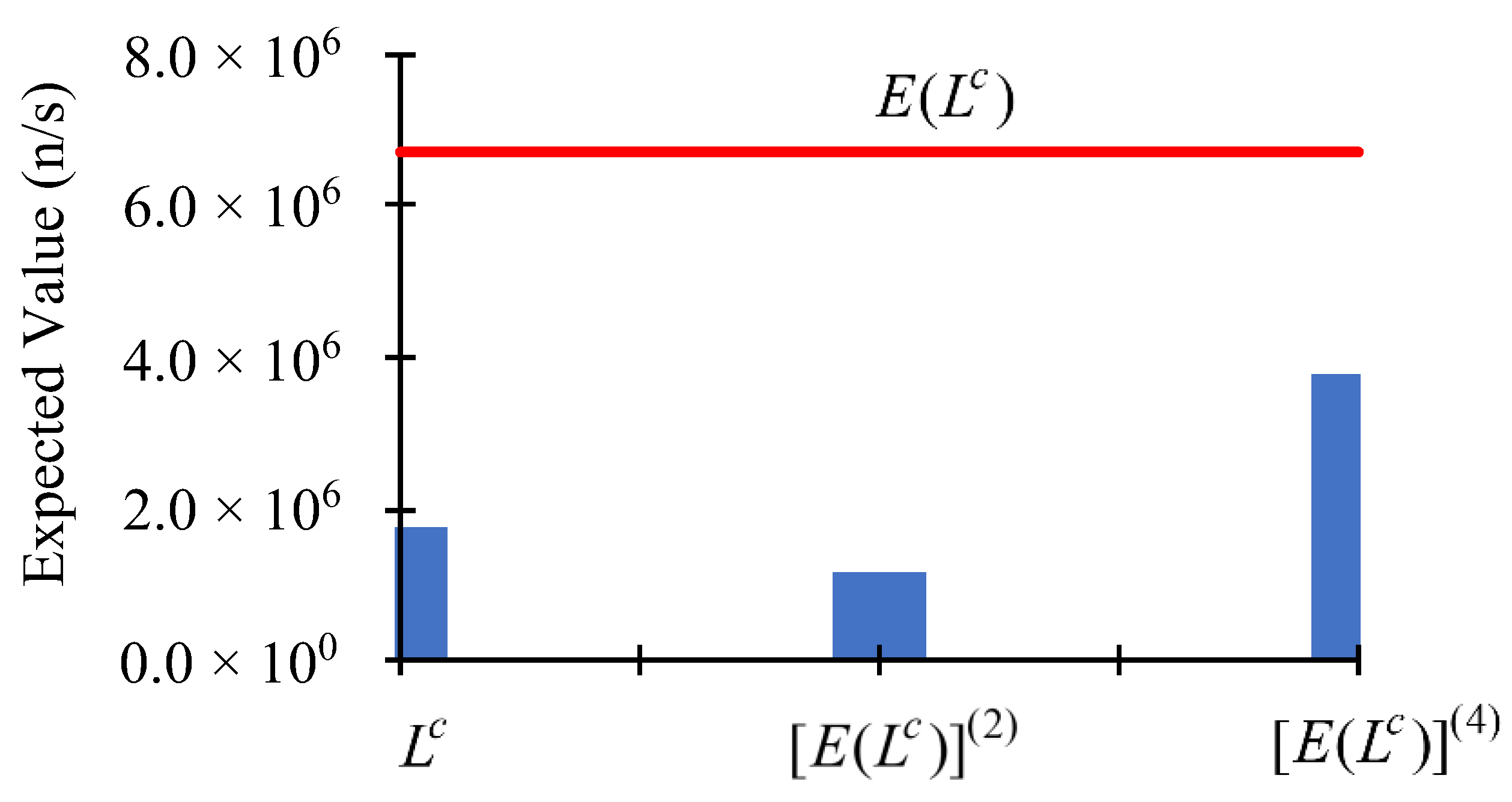
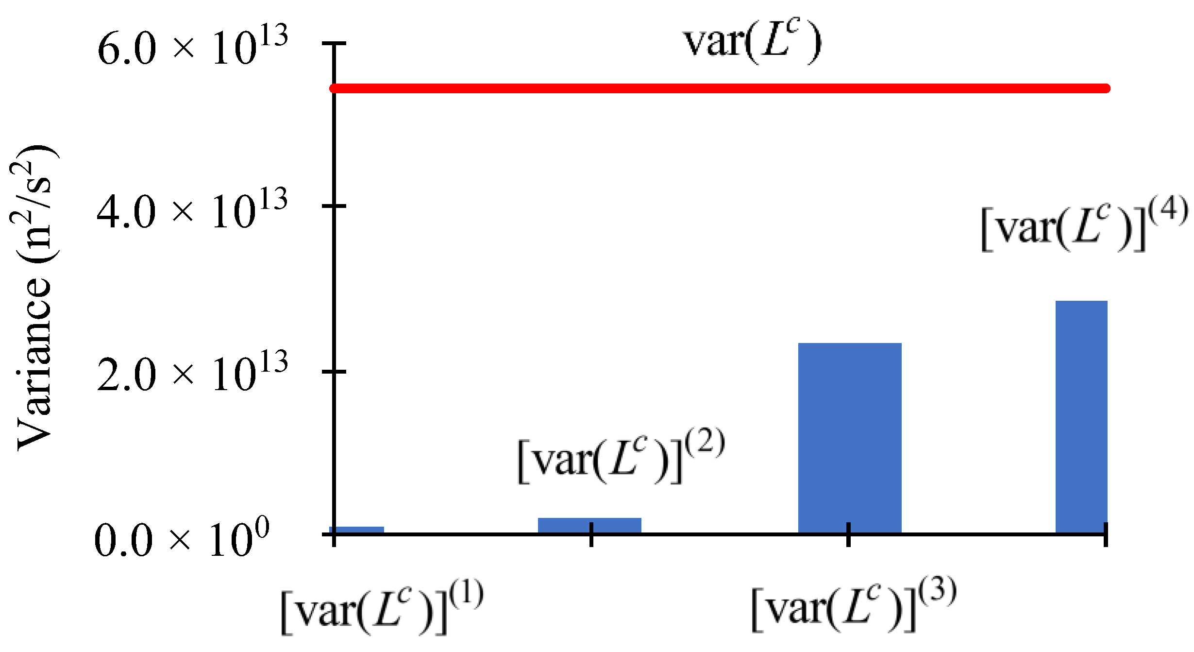
The results depicted in Figure 3 indicate that the contributions to

E (L^{c})

stemming from second-order sensitivities are smaller than those stemming from the zeroth-order term,

L^{c}

, but the contributions to

E (L^{c})

stemming from fourth-order sensitivities are larger than those stemming from the zeroth- and second-order terms. This oscillatory behavior with increasing amplitudes is indicative of the divergence of the Taylor-series underlying the computation of the expected value,

E (L^{c})

. The results depicted in Figure 4 for the variance,

var (L^{c})

, of the computed leakage response indicate that the contributions to

var (L^{c})

increase as the order of the contributing terms increase, thus underscoring the divergent nature of the underlying Taylor-series when the parameters have uniform relative standard deviations of 5%. On the other hand, relative standard deviation of 5% are often encountered in measurements of total cross sections, which highlights the need for computing the second and higher-order response sensitivities in order to investigate the convergence properties of the Taylor-series that underlies the determination of the statistics (expected values, variance, etc.) of the distribution of computed responses in the phase-space of imprecisely known model parameters.

3.3. Low Precision” parameters, Having Uniform Relative Standard Deviations

When considering uniform relative standard deviations of 10% for the uncorrelated and normally-distributed parameters (total cross sections), it has been shown by Cacuci and Fang [13] that the ratio of the 3^rd-order term with respect to the 2^nd-order term of the Taylor series is 1.93; the ratio of the 4^th-order term with respect to the 3^rd-order term of the Taylor series is 2.26. Both of these results are larger than 1.00, indicating that the Taylor-series presented in Eq. (1) would be divergent if used for parameters having standard deviations of 10%. The divergence of the Taylor-series for such parameter standard deviations is underscored by the corresponding results depicted in Figure 5 for the expected value,

E (L^{c})

, of the computed leakage response, which clearly indicate the massive increase of the contributions to

E (L^{c})

as the order of the retained terms increases. The conclusion that the Taylor-series expansion is divergent and should therefore not be used for parameters with uniform relative standard deviations

S D = 10 %

is reinforced by the corresponding results depicted in Figure 6 for the variance,

var (L^{c})

, of the computed leakage response. Figure 6 also highlights that the contributions to

var (L^{c})

increase massively as the order of the retained terms increases.

4. Concluding Discussion

This work has reviewed the fourth-order “sensitivity analysis” and “uncertainty quantification” aspects of computational models, the results of which are used as “input” into the 4^th-BERRU-PM methodology. The impact of combinations of sensitivities of increasingly higher order and various values for the standard deviations of the model’s parameters has been illustrated by using the PERP reactor physics benchmark. This benchmark is modeled by the neutron transport equation comprising 21,976 model parameters and is therefore representative of “large-scale” computational models of energy systems. It has been shown that the series-expansion representation of the expected value and variance of the computed leakage response is convergent and hence produces reliable results for normally-distributed parameters having uniform relative standard deviations of 2%. On the other hand, the series-expansion representations of the expected value and variance, respectively, become divergent for parameters having uniform relative standard deviations of 5%. This divergence becomes massive for parameters having uniform relative standard deviations of 10%.

In the accompanying Part 2 [17], the results obtained in this work will be combined, using the maximum entropy principle within the 4^th-BERRU-PM methodology, with the first four moments of the distribution of measured responses to obtain the best-estimate predicted mean value, standard deviation, skewness, and kurtosis for the neutron leakage response of the PERP benchmark, thereby illustrating the applicability of the 4^th-BERRU-PM methodology to improve the predictability and accuracy of models of energy systems.

Author Contributions

Conceptualization: D.G.C.; Investigation: R.F.; Writing—original draft: D.G.C.; Writing—review & editing: R.F. and D.G.C. All authors have read and agreed to the published version of the manuscript.

Funding

This research received no external funding

Data Availability Statement

All data are available in the main text.

Conflicts of Interest

The authors declare no conflict of interest.

Appendix A: Computational Model of the PERP Benchmark

The Polyethylene-Reflected Plutonium (acronym: PERP) reactor physics benchmark [2] is a one-dimensional spherical subcritical nuclear system driven by a source of spontaneous fission neutrons. The result (“response”) of interest for this benchmark is the neutron leakage out of the external surface of this benchmark. The computational model used for determining the neutron distribution within the benchmark and for determining the sensitivities (up to fourth-order) of the neutron leakage response with respect to the benchmark’s uncertain parameters has been presented in detail in the book by Cacuci and Fang [13]. The PERP benchmark comprises an inner sphere (designated as “material 1”) which is surrounded by a spherical shell (designated as “material 2”). The inner sphere of the PERP benchmark contains α-phase plutonium which acts as the source of particles; it has a radius

r_{1}

=3.794 cm. This inner sphere is surrounded by a spherical shell reflector made of polyethylene of thickness 3.81 cm; the radius of the outer shell containing polyethylene is

r_{s}

=7.604 cm. Table A1, below, specifies the constitutive materials of the PERP benchmark.

Table A1. Dimensions and Composition of the PERP Benchmark.

Materials	Isotopes	Weight Fraction	Density (g/cm³)	Zones
Material 1 (plutonium metal)	Isotope 1 (²³⁹Pu)	9.3804 × 10⁻¹	19.6	Material 1 is assigned to zone 1, which has a radius of 3.794 cm.
	Isotope 2 (²⁴⁰Pu)	5.9411 × 10⁻²
	Isotope 3 (⁶⁹Ga)	1.5152 × 10⁻³
	Isotope 4 (⁷¹Ga)	1.0346 × 10⁻³
Material 2 (polyethylene)	Isotope 5 (¹²C)	8.5630 × 10⁻¹	0.95	Material 2 is assigned to zone 2, which has an inner radius of 3.794 cm and an outer radius of 7.604 cm.
Material 2 (polyethylene)	Isotope 6 (¹H)	1.4370 × 10⁻¹	0.95

The neutron flux distribution within the PERP benchmark has been computed by using the deterministic software package PARTISN [20], which solves the standard multigroup approximation of the transport equation for the group-fluxes

φ^{g} (r, Ω)

, which can be written as follows:

B^{g} (α) φ^{g} (r, Ω) = Q^{g} (α; r), g = 1, \dots, G,

(A1)

φ^{g} (r_{s}, Ω) = 0, r_{s} \in S_{b}, Ω \cdot n < 0, g = 1, \dots, G,

(A2)

where:

\begin{array}{l} B^{g} (α) φ^{g} (r, Ω) ≜ Ω \cdot \nabla φ^{g} (r, Ω) + Σ_{t}^{g} (r) φ^{g} (r, Ω) \\ - \sum_{g^{'} = 1}^{G} \int_{4 π} Σ_{s}^{g^{'} \to g} (r, Ω^{'} \cdot Ω) φ^{g^{'}} (r, Ω^{'}) d Ω^{'} \\ - χ^{g} (r) \sum_{g^{'} = 1}^{G} \int_{4 π} {(ν Σ)}_{f}^{g^{'}} (r) φ^{g^{'}} (r, Ω^{'}) d Ω^{'}, \end{array}

(A3)

Q^{g} (α; r) ≜ \sum_{i = 1}^{N_{f}} λ_{i} N_{i, 1} F_{i}^{S F} ν_{i}^{S F} \frac{1}{I_{0}} \int_{E^{g + 1}}^{E^{g}} d E e^{- E / a_{i}} \sinh \sqrt{b_{i} E}, g = 1, \dots, G;

(A4)

with

I_{0} ≜ \frac{\sqrt{π {a_{i}}^{3} b_{i}}}{2} e^{\frac{a_{i} b_{i}}{4}} .

(A5)

In Eqs. (A4) and (A5), the subscript “

i

” denotes the number of nuclides within the spontaneous fission source.

Mathematically, the total neutron leakage from the PERP sphere, which is denoted as

L (α)

, will depend on all model parameters (indirectly, through the neutron flux) and it is defined, as follows:

L (α) ≜ \int_{V} d V \int_{0}^{\infty} d E \int_{Ω \cdot n > 0} d Ω Ω \cdot n δ (r - r_{s}) φ (r, E, Ω) = \int_{S_{b}} d S \sum_{g = 1}^{G} \int_{Ω \cdot n > 0} d Ω Ω \cdot n φ^{g} (r, Ω) .

(A6)

The PARTISN [20] computations used the MENDF71X library [21] which comprises 618-group cross sections. These cross-sections were collapsed to

G = 30

energy groups, with group boundaries,

E^{g}

, as presented in Table A2. The MENDF71X library [21] uses ENDF/B-VII.1 nuclear data [22]. The group boundaries,

E^{g}

, are user-defined and are therefore considered to be perfectly-well known parameters.

Table A2. Energy group structure, in [MeV], for PERP Benchmark computations.

g	1	2	3	4	5	6
$E^{g}$	1.50×10¹	1.35×10¹	1.20×10¹	1.00×10¹	7.79×10⁰	6.07×10⁰
$E^{g - 1}$	1.70×10¹	1.50×10¹	1.35×10¹	1.20×10¹	1.00×10¹	7.79×10⁰
g	7	8	9	10	11	12
$E^{g}$	3.68×10⁰	2.87×10⁰	2.23×10⁰	1.74×10⁰	1.35×10⁰	8.23×10⁻¹
$E^{g - 1}$	6.07× 10⁰	3.68×10⁰	2.87×10⁰	2.23×10⁰	1.74×10⁰	1.35×10⁰
g	13	14	15	16	17	18
$E^{g}$	5.00×10⁻¹	3.03×10⁻¹	1.84×10⁻¹	6.76×10⁻²	2.48×10⁻²	9.12×10⁻³
$E^{g - 1}$	8.23×10⁻¹	5.00×10⁻¹	3.03×10⁻¹	1.84×10⁻¹	6.76×10⁻²	2.48×10⁻²
g	19	20	21	22	23	24
$E^{g}$	3.35×10⁻³	1.24×10⁻³	4.54×10⁻⁴	1.67×10⁻⁴	6.14×10⁻⁵	2.26×10⁻⁵
$E^{g - 1}$	9.12×10⁻³	3.35×10⁻³	1.24×10⁻³	4.54×10⁻⁴	1.67×10⁻⁴	6.14×10⁻⁵
g	25	26	27	28	29	30
$E^{g}$	8.32×10⁻⁶	3.06×10⁻⁶	1.13×10⁻⁶	4.14×10⁻⁷	1.52×10⁻⁷	1.39×10⁻¹⁰
$E^{g - 1}$	2.26×10⁻⁵	8.32×10⁻⁶	3.06×10⁻⁶	1.13×10⁻⁶	4.14×10⁻⁷	1.52×10⁻⁷

The source of neutrons in the PERP benchmark is provided by the spontaneous fissions stemming from ²³⁹Pu (Isotope 1) and ²⁴⁰Pu (Isotope 2); there are no delayed neutron or

(α, n)

sources. The spontaneous fission source has been computed using the code SOURCES4C [23]. For an actinide nuclide

k

, where

k = 1, 2

for the PERP benchmark, the spontaneous source depends on the following 12 model parameters: the decay constant

λ_{k}

, the atom density

N_{k, m}

, the average number of neutrons per spontaneous fission

ν_{k}^{S F}

, the spontaneous fission branching ratio

F_{k}^{S F}

, and the two parameters

a_{k}

and

b_{k}

used in a Watt’s fission spectrum to approximate the spontaneous fission neutron spectrum. The nominal values of these parameters (except for

N_{k, m}

) are available from a library file contained in SOURCES4C [23], while the nominal values for

N_{k, m}

are specified from the PERP benchmark. These imprecisely known source parameters also contribute to the accuracy of the neutron transport calculation.

PARTISN [20] uses the discrete-ordinates approximation to discretize the angular variable in the first and second terms on the right-side of Eq. (A4), and it uses a finite-moments expansion in spherical harmonics to approximate the angular variable in the third and fourth terms on the right side of Eq. (A4). The specific computations in this work were performed while using a P₃ Legendre expansion of the scattering cross section, an angular quadrature of S₂₅₆, and a fine-mesh spacing of 0.005 cm (comprising 759 meshes for the plutonium sphere of radius of 3.794 cm, and 762 meshes for the polyethylene shell of thickness of 3.81 cm). It is convenient to retain the continuous representation in the angular and radial variables since the spatial and angular discretization parameters are considered to be perfectly well known. The various quantities in Eqs. (A1)−(A5) have their usual meanings for the standard form of the multigroup neutron transport equation, as follows:

Using the notation employed in PARTISN [20], the quantity $φ^{g} (r, Ω) ≜ \int_{E^{g - 1 / 2}}^{E^{g + 1 / 2}} φ (r, E, Ω) d E$ denotes the “group-flux” for group $g$ , and is the unknown state-function obtained by solving Eqs. (A1) and (A2).
The spontaneous-fission isotopes in the PERP benchmark are “isotope 1” (²³⁹Pu) and “isotope 2” (²⁴⁰Pu). The quantity $N_{f}$ denotes the total number of spontaneous-fission isotopes; for the PERP benchmark, $N_{f} = 2$ . The spontaneous fission neutron spectra of ²³⁹Pu and, respectively, ²⁴⁰Pu, are approximated by Watt’s fission spectra, each spectrum using two evaluated parameters, denoted as $a_{k}$ and $b_{k}$ , respectively. The decay constant for actinide nuclide $k$ is denoted as $λ_{k}$ , while $F_{k}^{S F}$ denotes the fraction of decays that are spontaneous fission (the “spontaneous fission branching fraction”).
The quantity $N_{i, m}$ denotes the atom density of isotope i in material m; $i = 1, \dots, I$ , $m = 1, \dots, M$ , where $I$ denotes the total number of isotopes, and $M$ denotes the total number of materials. The computation of $N_{i, m}$ uses the following well-known expression:

$N_{i, m} ≜ \frac{ρ_{m} w_{i, m} N_{A}}{A_{i}},$

(A7)

where $ρ_{m}$ denotes the mass density of material m, $m = 1, \dots, M$ ; $w_{i, m}$ denotes the weight fraction of isotope i in material m; $A_{i}$ denotes the atomic weight of isotope $i$ , $i = 1, \dots, I$ ; $N_{A}$ denotes the Avogadro’s number. For the PERP benchmark, $I = 6$ and $M = 2$ , but since the respective isotopes are all distinct (i.e., are not repeated) in the PERP benchmark’s distinct materials, as specified in Table A1, it follows that only the following isotopic number densities exist for this benchmark: $N_{1, 1}, N_{2, 1}, N_{3, 1}, N_{4, 1}, N_{5, 2}, N_{6, 2}$ .
The quantity $Σ_{s}^{g^{'} \to g} (r, Ω^{'} \cdot Ω)$ represents the scattering transfer cross section from energy group $g', g' = 1, \dots, G$ into energy group $g, g = 1, \dots, G$ . The transfer cross sections is computed in terms of the $l$ ^th-order Legendre coefficients $σ_{s, l, i}^{g^{'} \to g}$ (of the Legendre-expanded microscopic scattering cross section from energy group $g^{'}$ into energy group $g$ , for isotope $i$ ), which are tabulated parameters, using the following finite-order expansion:

$\begin{array}{l} Σ_{s}^{g^{'} \to g} (r, Ω^{'} \cdot Ω) = \sum_{m = 1}^{M = 2} Σ_{s, m}^{g^{'} \to g} (r, Ω^{'} \cdot Ω), \\ Σ_{s, m}^{g^{'} \to g} (r, Ω^{'} \cdot Ω) ≅ \sum_{i = 1}^{I = 6} N_{i, m} \sum_{l = 0}^{I S C T = 3} (2 l + 1) σ_{s, l, i}^{g^{'} \to g} (r) P_{l} (Ω^{'} \cdot Ω), m = 1, 2, \end{array}$

(A8)

where $I S C T = 3$ denotes the order of the respective finite expansion in Legendre polynomial. The variable $r$ will henceforth no longer appear in the arguments of the various cross sections since the cross-sections for every material are treated in the PARTISN [20] computations as being space-independent within the respective material.
The total cross section $Σ_{t}^{g}$ for energy group $g, g = 1, \dots, G,$ and material $m$ , is computed for the PERP benchmark using the following expression:

$Σ_{t}^{g} = \sum_{m = 1}^{M = 2} Σ_{t, m}^{g}; Σ_{t, m}^{g} = \sum_{i}^{I} N_{i, m} σ_{t, i}^{g} = \sum_{i}^{I} N_{i, m} [σ_{f, i}^{g} + σ_{c, i}^{g} + \sum_{g^{'} = 1}^{G} σ_{s, l = 0, i}^{g \to g^{'}}], m = 1, 2,$

(A9)

where $σ_{f, i}^{g}$ and $σ_{c, i}^{g}$ denote, respectively, the tabulated group microscopic fission and neutron capture cross sections for group $g, g = 1, \dots, G$ . Other nuclear reactions, including (n,2n) and (n,3n) reactions, are not present in this benchmark. The expressions in Eqs. (A8) and (A9) indicate that the zeroth-order (i.e., $l = 0$ ) scattering cross sections must be separately considered from the higher order (i.e., $l \geq 1$ ) scattering cross sections, since the former contribute to the total cross sections, while the latter do not.
PARTISN [20] computes the quantity ${(ν Σ_{f})}^{g}$ using the quantities ${(ν σ)}_{f, i}^{g}$ , which are provided in data files for each isotope $i$ , and energy group $g$ , as follows:

${(ν Σ_{f})}^{g} = \sum_{m = 1}^{M = 2} {(ν Σ_{f})}_{m}^{g}; {(ν Σ_{f})}_{m}^{g} = \sum_{i = 1}^{I = 6} N_{i, m} {(ν σ_{f})}_{i}^{g}, m = 1, 2.$

(A10)

For the purposes of sensitivity analysis, the quantity $ν_{i}^{g}$ , which denotes the number of neutrons that were produced per fission by isotope $i$ and energy group $g$ , can be obtained by using the relation $ν_{i}^{g} = {(ν σ_{f})}_{i}^{g} / σ_{f, i}^{g}$ , where the isotopic fission cross sections $σ_{f, i}^{g}$ are available in data files for computing reaction rates.
The quantity $χ^{g}$ denotes the fission spectrum in energy group $g$ ; it is defined in PARTISN [20] as a space-independent quantity, as follows:

$χ^{g} ≜ \frac{\sum_{i = 1}^{N_{f}} χ_{i}^{g} N_{i, m} \sum_{g^{'} = 1}^{G} {(ν σ_{f})}_{i}^{g^{'}} f_{i}^{g^{'}}}{\sum_{i = 1}^{N_{f}} N_{i, m} \sum_{g^{'} = 1}^{G} {(ν σ_{f})}_{i}^{g^{'}} f_{i}^{g^{'}}}, w i t h \sum_{g = 1}^{G} χ_{i}^{g} = 1,$

(A11)

where $χ_{i}^{g}$ denotes the isotopic fission spectrum in group $g$ , while $f_{i}^{g}$ denotes the corresponding spectrum weighting function.
The vector $α$ , which appears in the expression of the Boltzmann-operator $B^{g} (α)$ , represents the “vector of imprecisely known model parameters,” comprising 21,976 components, which are presented in Table A3, below.

Table A3. Summary of imprecisely known parameters for the PERP benchmark.

Symbol	Parameter Name	Number of Parameters
$σ_{t, i}^{g}$	Multigroup microscopic total cross section for isotope $i$ and energy group $g$	180 $f o r i = 1, \dots, 6; g = 1, \dots, 30$
$σ_{s, l, i}^{g' \to g}$	Multigroup microscopic scattering cross section for $l$ -th order Legendre expansion, from energy group $g^{'}$ into energy group $g$ , for isotope $i$	21,600 $\begin{array}{l} f o r l = 0, \dots, 3; i = 1, \dots, 6; \\ g, g^{'} = 1, \dots, 30 \end{array}$
$σ_{f, i}^{g}$	Multigroup microscopic fission cross section $i$ and energy group $g$	60 $f o r i = 1, 2; g = 1, \dots, 30$
$ν_{i}^{g}$	Average number of neutrons per fission for isotope $i$ and energy group $g$	60 $f o r i = 1, 2; g = 1, \dots, 30$
$χ_{i}^{g}$	Fission spectrum for isotope $i$ and energy group $g$	60 $f o r i = 1, 2; g = 1, \dots, 30$
$q_{j}$	Source parameters $λ_{1}, λ_{2}; F_{1}^{S F}, F_{2}^{S F};$ $a_{1}, a_{2}; b_{1}, b_{2}; ν_{1}^{S F}, ν_{2}^{S F}$	10
$N_{i, m}$	Isotopic number density for isotope $i$ and material $m$	6 $N_{1, 1}, N_{2, 1}, N_{3, 1}, N_{4, 1}, N_{5, 2}, N_{6, 2}$
$J_{α}$	Total number of parameters:	21,976

In view of Eq. (A9), the total cross section

Σ_{t}^{g} \to Σ_{t}^{g} (t)

is characterized by the following vectors of uncertain parameters:

N ≜ {[n_{1}, \dots, n_{J_{n}}]}^{†} ≜ {[N_{1, 1}, N_{2, 1}, N_{3, 1}, N_{4, 1}, N_{5, 2}, N_{6, 2}]}^{†}, J_{n} = 6,

(A12)

\begin{array}{l} σ_{t} ≜ {[t_{1}, \dots, t_{J_{σ t}}]}^{†} ≜ {[σ_{t, i = 1}^{1}, σ_{t, i = 1}^{2}, \dots, σ_{t, i = 1}^{G}, \dots, σ_{t, i}^{g}, \dots, σ_{t, i = I}^{1}, \dots, σ_{t, i = I}^{G}]}^{†}, \\ i = 1, \dots, I; g = 1, \dots, G; J_{σ t} = I \times G . \end{array}

(A13)

In Eqs. (A12) and (A13), the dagger “

†

” denotes “transposition”,

σ_{t, i}^{g}

denotes the microscopic total cross section for isotope

i

and energy group

g

N_{i, m}

denotes the respective isotopic number density, and

J_{n}

denotes the total number of isotopic number densities in the model.

In view of Eq. (A8), the scattering cross section

Σ_{s}^{g^{'} \to g} (Ω^{'} \cdot Ω) \to Σ_{s}^{g^{'} \to g} (s; Ω^{'} \cdot Ω)

is characterized by the following vector of uncertain parameters:

\begin{array}{l} σ_{s} ≜ {[s_{1}, \dots, s_{J_{σ s}}]}^{†} ≜ [σ_{s, l = 0, i = 1}^{g' = 1 \to g = 1}, \dots, σ_{s, l = 0, i = 1}^{g' = G \to g = 1}, σ_{s, l = 0, i = 1}^{g' = 1 \to g = 2}, {\dots, σ_{s, l, i}^{g' \to g}, \dots, σ_{s, I S C T, i = I}^{G \to G}]}^{†}, \\ l = 0, \dots, I S C T; i = 1, \dots, I; g, g^{'} = 1, \dots, G; J_{σ s} = (G \times G) \times I \times (I S C T + 1) . \end{array}

(A14)

In view of Eq. (A10), the quantity

{(ν Σ_{f})}^{g} \to {[ν Σ_{f} (f)]}^{g}

in the fission integral

\int_{4 π} {(ν Σ)}_{f}^{g^{'}} φ^{g^{'}} (r, Ω^{'}) d Ω^{'}

depends on the following vector of uncertain parameters:

\begin{array}{l} σ_{f} ≜ {[σ_{f, i = 1}^{1}, σ_{f, i = 1}^{2}, \dots, σ_{f, i = 1}^{G}, \dots, σ_{f, i}^{g}, \dots, σ_{f, i = N_{f}}^{1}, \dots, σ_{f, i = N_{f}}^{G}]}^{†}, \\ i = 1, \dots, N_{f}; g = 1, \dots, G; J_{σ f} = G \times N_{f} . \end{array}

(A15)

\begin{array}{l} ν ≜ {[ν_{i = 1}^{1}, ν_{i = 1}^{2}, \dots, ν_{i = 1}^{G}, \dots, ν_{i}^{g}, \dots, ν_{i = N_{f}}^{1}, \dots, ν_{i = N_{f}}^{G}]}^{†} \\ ≜ {[f_{J_{σ f} + 1}, \dots, f_{J_{σ f} + J_{ν}}]}^{†}, i = 1, \dots, N_{f}; g = 1, \dots, G; J_{ν} = G \times N_{f}, \end{array}

(A16)

and where

σ_{f, i}^{g}

denotes the microscopic fission cross section for isotope

i

and energy group

g

ν_{i}^{g}

denotes the average number of neutrons per fission for isotope

i

and energy group

g

, and

N_{f}

denotes the total number of fissionable isotopes.

The fission spectrum is considered to depend on the following vector of uncertain parameters:

p ≜ {[χ_{i = 1}^{g = 1}, χ_{i = 1}^{g = 2}, \dots, χ_{i = 1}^{G}, \dots, χ_{i}^{g}, \dots, χ_{N_{f}}^{G}]}^{†}, i = 1, \dots, N_{f}; g = 1, \dots, G; J_{p} = G \times N_{f} .

(A17)

In view of Eq. (A11), the quantities

χ^{g}

depend, in turn, on the parameters

χ_{i}^{g}

N_{i, m},

f_{i}^{g}

{(ν σ_{f})}_{i}^{g}

, but these latter dependences can be taken into account by applying the chain rule to the 1^st-order sensitivities

\partial L / \partial χ^{g}

, after these sensitivities have been obtained.

In view of Eq. (A4), the source

Q^{g} (r) \to Q^{g} (q; N)

depends on the following vector of uncertain parameters:

q ≜ {[λ_{1}, λ_{2}; F_{1}^{S F}, F_{2}^{S F}; a_{1}, a_{2}; b_{1}, b_{2}; ν_{1}^{S F}, ν_{2}^{S F}]}^{†}, J_{q} = 10.

(A18)

In view of Eqs. (A12)–(A18), the model parameters characterizing the PERP benchmark can all be considered to be the components of the “vector of model parameters”

α

which is defined below:

α ≜ {[α_{1}, \dots, α_{J_{α}}]}^{†} ≜ {[σ_{t}; σ_{s}; σ_{f}; ν; p; q; N]}^{†}, J_{α} = J_{σ t} + J_{σ s} + J_{σ f} + J_{ν} + J_{p} + J_{q} + J_{n} .

(A19)

Thus, the PERP benchmark comprises a total of

J_{α} = (I \times G) + (G \times G) \times I \times (I S C T + 1) + 2 (G \times N_{f}) + G \times N_{f} + 10 + 6 = 21, 976.

imprecisely known (i.e., uncertain) model parameters, as summarized in Table A3. Although the numerical model of the PERP benchmark comprises 21,976 uncertain parameters, only 7,477 parameters have nonzero nominal values, as follows: 180 group-averaged total microscopic cross sections, 7,101 non-zero group-averaged scattering microscopic cross sections (the other scattering cross sections, of which there are 21,600 in total, are zero); 120 fission process parameters; 60 fission spectrum parameters; 10 parameters describing the experiment’s nuclear sources; and 6 isotopic number densities.

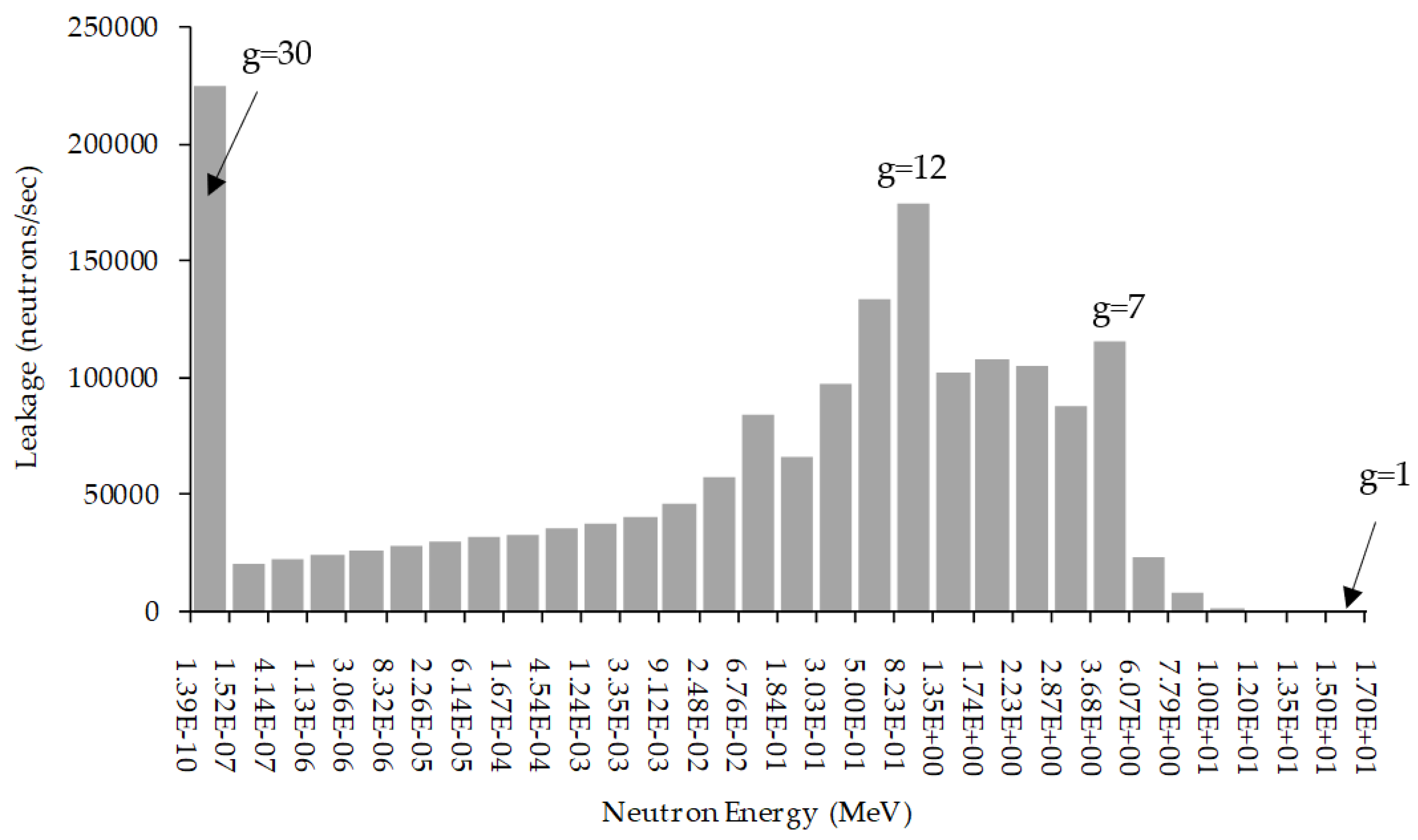
The nominal value of total leakage, computed by using Eq. (A6) at the nominal parameter values (which are denoted using the usual notation

α^{0}

L (α^{0}) = 1.7648 \times 10^{6}

neutrons/sec. Figure A1, below, depicts the histogram plot of the leakage for each energy group for the PERP benchmark.

Figure A1. Histogram plot of the energy-dependent leakage for the PERP benchmark.

References

Cacuci, D.G. Fourth-Order Predictive Modelling: II. 4th-BERRU-PM Methodology for Combining Measurements with Computations to Obtain Best-Estimate Results with Reduced Uncertainties. Am. J. Comp. Math., 2023, 13, 439-475. [CrossRef]
Valentine, T.E. Polyethylene-Reflected Plutonium Metal Sphere Subcritical Noise Measurements. SUB-PU-METMIXED-001, International Handbook of Evaluated Criticality Safety Benchmark Experiments; NEA/NSC/DOC(95)03/I-IX; Organization for Economic Co-Operation and Development; Nuclear Energy Agency: Paris, France, 2006.
Jaynes, E.T. Information Theory and Statistical Mechanics. Phys. Rev., 1957, 106, pp. 620.
Cacuci, D.G. Second-Order MaxEnt Predictive Modelling Methodology. I: Deterministically Incorporated Computational Model (2nd-BERRU-PMD). Am. J. Comp. Math., 2013, 13, 236-266. [CrossRef]
Cacuci, D.G. Second-Order MaxEnt Predictive Modelling Methodology. II: Probabilistically Incorporated Computational Model (2nd-BERRU-PMP). Am. J. Comp. Math., 2023, 13, 267-294. [CrossRef]
SCALE: a modular code system for performing standardized computer analyses for licensing evaluation, ORNL/TM 2005/39, Version 6, Oak Ridge National Laboratory, Oak Ridge, Tennessee, USA, 2009.
Venard, C.; Santamarina, A.; Leclainche, A.; Mournier, C. The R.I.B. Tool for the determination of computational bias and associated uncertainty in the CRISTAL criticality safety package. Proceedings of ANS Nuclear Criticality Safety Division Topical Meeting (NCSD 2009), Richland, Washington, USA, 2009.
Rabier, F. Overview of global data assimilation developments in numerical weather-prediction centers, Q. J. R. Meteorol. Soc., 2005, 131(613), 3215.
Lewis, J. M.; Lakshmivarahan, S.; Dhall, S.K. Dynamic Data Assimilation: A Least Square Approach. Cambridge University Press, Cambridge, UK, 2006.
Lahoz, W.; Khattatov, B.; Ménard, R. Eds. Data Assimilation: Making Sense of Observations, Springer Verlag, Heidelberg, Germany, 2010.
Práger, T.; Kelemen, F. D. Adjoint methods and their application in earth sciences. Chapter 4, Part A, pp 203-275, in Faragó, I.; Havasi, Á.; Zlatev, Z. (Eds.) Advanced Numerical Methods for Complex Environmental Models: Needs and Availability, Bentham Science Publishers, Bussum, The Netherlands, 2013.
Cacuci, D.G.; Navon, M.I.; Ionescu-Bujor, M. Computational Methods for Data Evaluation and Assimilation. Chapman & Hall/CRC, Boca Raton, USA, 2014.
Cacuci, D. G.; Fang, R. The nth-Order Comprehensive Adjoint Sensitivity Analysis Methodology: Overcoming the Curse of Dimensionality: Vol. II: Application to a Large-Scale System; Springer Nature Switzerland AG, 6330 Cham, Switzerland, 2023. ISBN 978-3-031-19634-8 ISBN 978-3-031-19635-5. [CrossRef]
Cacuci, D.G. The nth-Order Comprehensive Adjoint Sensitivity Analysis Methodology: Overcoming the Curse of Dimensionality. Volume I: Linear Systems. Springer Nature Switzerland, Cham, Switzerland, 2022. [CrossRef]
Cacuci, D. G. The nth-Order Comprehensive Adjoint Sensitivity Analysis Methodology (nth-CASAM): Overcoming the Curse of Dimensionality in Sensitivity and Uncertainty Analysis, Volume III: Nonlinear Systems. Springer Nature Switzerland, Cham, 2023. [CrossRef]
Bellman, R.E. Dynamic programming. Rand Corporation, Princeton University Press, ISBN 978-0-691-07951-6, USA. 1957.
Cacuci, D. G.; Fang, R. Review of Fourth-Order Maximum Entropy Based Predictive Modelling and Illustrative Application to a Nuclear Reactor Benchmark: II. Best-Estimate Predicted Values and Uncertainties for Model Responses and Parameters. Energies, 2024, submitted.
Tukey, J.W. The Propagation of Errors, Fluctuations and Tolerances. Technical Reports No. 10–12; Princeton University. Princeton, NJ, USA, 1957.
Saltarelli, A.; Chan, K.; Scott, E. M. (Eds.) Sensitivity analysis. J. Wiley & Sons Ltd. Chichester, UK, 2000.
Alcouffe, R. E.; Baker, R. S.; Dahl, J. A.; Turner, S.A.; Ward, R. PARTISN: A Time-Dependent, Parallel Neutral Particle Transport Code System. LA-UR-08-07258; Los Alamos National Laboratory: Los Alamos, NM, USA, 2008.
Conlin, J.L.; Parsons, D.K.; Gardiner, S.J.; Gray, M.; Lee, M.B.; White, M.C. MENDF71X: Multigroup Neutron Cross-Section Data Tables Based upon ENDF/B-VII.1X. Los Alamos National Laboratory Report LA-UR-15-29571; Los Alamos National Laboratory: Los Alamos, NM, USA, 2013.
Chadwick M.B.; Herman M.; Obložinský P.; Dunn M.E.; Danon Y.; Kahler A.C.; Smith D.L.; Pritychenko B.; Arbanas G.; Brewer R. et al. ENDF/B-VII.1: Nuclear data for science and technology: Cross sections, covariances, fission product yields and decay data. Nucl. Data Sheets, 2011, 112, 2887–2996. [CrossRef]
Wilson, W.B.; Perry, R.T.; Shores, E.F.; Charlton, W.S.; Parish, T.A.; Estes, G.P.; Brown, T.H.; Arthur, E.D.; Bozoian, M.; England, T.R.; et al. SOURCES4C: A code for calculating (α,n), spontaneous fission, and delayed neutron sources and spectra. In Proceedings of the American Nuclear Society/Radiation Protection and Shielding Division 12th Biennial Topical Meeting, Santa Fe, NM, USA, 14–18 April 2002.

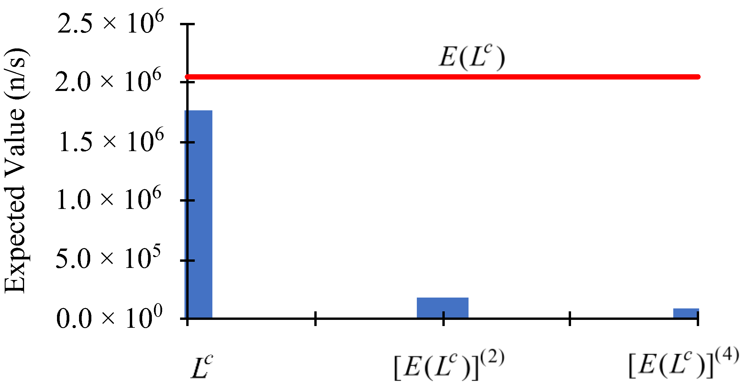
Figure 1. Contributions to the expected value,

E (L^{c})

, of the computed leakage response from parameters having uniform relative standard deviations

S D = 2 %

: (i) zeroth-order:

L^{c}

; (ii) second-order:

{[E (L^{c})]}^{(2)}

; (iii) fourth-order:

{[E (L^{c})]}^{(4)}

; (iv) the odd-order contributions are null.

Figure 1. Contributions to the expected value,

E (L^{c})

, of the computed leakage response from parameters having uniform relative standard deviations

S D = 2 %

: (i) zeroth-order:

L^{c}

; (ii) second-order:

{[E (L^{c})]}^{(2)}

; (iii) fourth-order:

{[E (L^{c})]}^{(4)}

; (iv) the odd-order contributions are null.

Figure 2. Contributions to the variance,

var (L^{c})

, of the computed leakage response from parameters having uniform relative standard deviations

S D = 2 %

: (i) first-order:

{[var (L^{c})]}^{(1)}

; (ii) second-order:

{[var (L^{c})]}^{(2)}

; (iii) third-order:

{[var (L^{c})]}^{(3)}

; (iv) fourth-order:

{[var (L^{c})]}^{(4)}

Figure 2. Contributions to the variance,

var (L^{c})

, of the computed leakage response from parameters having uniform relative standard deviations

S D = 2 %

: (i) first-order:

{[var (L^{c})]}^{(1)}

; (ii) second-order:

{[var (L^{c})]}^{(2)}

; (iii) third-order:

{[var (L^{c})]}^{(3)}

; (iv) fourth-order:

{[var (L^{c})]}^{(4)}

Figure 3. Contributions to the expected value,

E (L^{c})

, of the computed leakage response from parameters having uniform relative standard deviations

S D = 5 %

: (i) zeroth-order:

L^{c}

; (ii) second-order:

{[E (L^{c})]}^{(2)}

; (iii) fourth-order:

{[E (L^{c})]}^{(4)}

; (iv) the odd-order contributions are null.

Figure 3. Contributions to the expected value,

E (L^{c})

, of the computed leakage response from parameters having uniform relative standard deviations

S D = 5 %

: (i) zeroth-order:

L^{c}

; (ii) second-order:

{[E (L^{c})]}^{(2)}

; (iii) fourth-order:

{[E (L^{c})]}^{(4)}

; (iv) the odd-order contributions are null.

Figure 4. Contributions to the variance,

var (L^{c})

, of the computed leakage response from parameters having uniform relative standard deviations

S D = 5 %

: (i) first-order:

{[var (L^{c})]}^{(1)}

; (ii) second-order:

{[var (L^{c})]}^{(2)}

; (iii) third-order:

{[var (L^{c})]}^{(3)}

; (iv) fourth-order:

{[var (L^{c})]}^{(4)}

Figure 4. Contributions to the variance,

var (L^{c})

, of the computed leakage response from parameters having uniform relative standard deviations

S D = 5 %

: (i) first-order:

{[var (L^{c})]}^{(1)}

; (ii) second-order:

{[var (L^{c})]}^{(2)}

; (iii) third-order:

{[var (L^{c})]}^{(3)}

; (iv) fourth-order:

{[var (L^{c})]}^{(4)}

Figure 5. Contributions to the expected value,

E (L^{c})

, of the computed leakage response from parameters having uniform relative standard deviations

S D = 10 %

: (i) zeroth-order:

L^{c}

; (ii) second-order:

{[E (L^{c})]}^{(2)}

; (iii) fourth-order:

{[E (L^{c})]}^{(4)}

; (iv) the odd-order contributions are null.

Figure 5. Contributions to the expected value,

E (L^{c})

, of the computed leakage response from parameters having uniform relative standard deviations

S D = 10 %

: (i) zeroth-order:

L^{c}

; (ii) second-order:

{[E (L^{c})]}^{(2)}

; (iii) fourth-order:

{[E (L^{c})]}^{(4)}

; (iv) the odd-order contributions are null.

Figure 6. Contributions to the variance,

var (L^{c})

, of the computed leakage response from parameters having uniform relative standard deviations

S D = 10 %

: (i) first-order:

{[var (L^{c})]}^{(1)}

; (ii) second-order:

{[var (L^{c})]}^{(2)}

; (iii) third-order:

{[var (L^{c})]}^{(3)}

; (iv) fourth-order:

{[var (L^{c})]}^{(4)}

Figure 6. Contributions to the variance,

var (L^{c})

, of the computed leakage response from parameters having uniform relative standard deviations

S D = 10 %

: (i) first-order:

{[var (L^{c})]}^{(1)}

; (ii) second-order:

{[var (L^{c})]}^{(2)}

; (iii) third-order:

{[var (L^{c})]}^{(3)}

; (iv) fourth-order:

{[var (L^{c})]}^{(4)}

Table 1. Comparison of the unmixed relative sensitivities,

S^{(1)} (σ_{t, 6}^{g})

S^{(2)} (σ_{t, 6}^{g}, σ_{t, 6}^{g})

S^{(3)} (σ_{t, 6}^{g}, σ_{t, 6}^{g}, σ_{t, 6}^{g})

, and

S^{(4)} (σ_{t, 6}^{g}, σ_{t, 6}^{g}, σ_{t, 6}^{g}, σ_{t, 6}^{g})

g = 1, \dots, 30

, for isotope 6 (¹H).

Table 1. Comparison of the unmixed relative sensitivities,

S^{(1)} (σ_{t, 6}^{g})

S^{(2)} (σ_{t, 6}^{g}, σ_{t, 6}^{g})

S^{(3)} (σ_{t, 6}^{g}, σ_{t, 6}^{g}, σ_{t, 6}^{g})

, and

S^{(4)} (σ_{t, 6}^{g}, σ_{t, 6}^{g}, σ_{t, 6}^{g}, σ_{t, 6}^{g})

g = 1, \dots, 30

, for isotope 6 (¹H).

g	1^st-order	2^nd-order	3^rd-order	4^th-order
1	−8.471 × 10⁻⁶	7.636 × 10⁻⁷	6.322 × 10⁻⁸	1.460 × 10⁻⁷
2	−2.060 × 10⁻⁵	2.280 × 10⁻⁶	4.516 × 10⁻⁸	4.956 × 10⁻⁷
3	−6.810 × 10⁻⁵	9.021 × 10⁻⁶	−4.677 × 10⁻⁷	2.245 × 10⁻⁶
4	−3.932 × 10⁻⁴	6.673 × 10⁻⁵	−8.758 × 10⁻⁶	2.039 × 10⁻⁵
5	−2.449 × 10⁻³	5.549 × 10⁻⁴	−1.216 × 10⁻⁴	2.142 × 10⁻⁴
6	−9.342 × 10⁻³	2.935 × 10⁻³	−1.123 × 10⁻³	1.553 × 10⁻³
7	−7.589 × 10⁻²	3.949 × 10⁻²	−2.690 × 10⁻²	3.513 × 10⁻²
8	−9.115 × 10⁻²	5.604 × 10⁻²	−4.380 × 10⁻²	5.536 × 10⁻²
9	−1.358 × 10⁻¹	1.014 × 10⁻¹	−9.758 × 10⁻²	1.416 × 10⁻¹
10	−1.659 × 10⁻¹	1.428 × 10⁻¹	−1.604 × 10⁻¹	2.582 × 10⁻¹
11	−1.899 × 10⁻¹	1.849 × 10⁻¹	−2.385 × 10⁻¹	4.233 × 10⁻¹
12	−4.446 × 10⁻¹	6.620 × 10⁻¹	−1.373 × 10⁰	3.815 × 10⁰
13	−5.266 × 10⁻¹	9.782 × 10⁻¹	−2.590 × 10⁰	9.015 × 10⁰
14	−5.772 × 10⁻¹	1.262 × 10⁰	−3.991 × 10⁰	1.650 × 10¹
15	−5.820 × 10⁻¹	1.391 × 10⁰	−4.581 × 10⁰	2.208 × 10¹
16	−1.164 × 10⁰	4.460 × 10⁰	−2.530 × 10¹	1.890 × 10²
17	−1.173 × 10⁰	4.853 × 10⁰	−2.991 × 10¹	2.432 × 10²
18	−1.141 × 10⁰	4.828 × 10⁰	−3.049 × 10¹	2.543 × 10²
19	−1.094 × 10⁰	4.619 × 10⁰	−2.913 × 10¹	2.428 × 10²
20	−1.033 × 10⁰	4.284 × 10⁰	−2.655 × 10¹	2.175 × 10²
21	−9.692 × 10⁻¹	3.937 × 10⁰	−2.388 × 10¹	1.915 × 10²
22	−8.917 × 10⁻¹	3.515 × 10⁰	−2.069 × 10¹	1.609 × 10²
23	−8.262 × 10⁻¹	3.177 × 10⁰	−1.823 × 10¹	1.382 × 10²
24	−7.495 × 10⁻¹	2.792 × 10⁰	−1.552 × 10¹	1.140 × 10²
25	−7.087 × 10⁻¹	2.604 × 10⁰	−1.427 × 10¹	1.033 × 10²
26	−6.529 × 10⁻¹	2.349 × 10⁰	−1.260 × 10¹	8.932 × 10¹
27	−5.845 × 10⁻¹	2.039 × 10⁰	−1.061 × 10¹	7.288 × 10¹
28	−5.474 × 10⁻¹	1.885 × 10⁰	−9.678 × 10⁰	6.565 × 10¹
29	−5.439 × 10⁻¹	1.891 × 10⁰	−9.800 × 10⁰	6.705 × 10¹
30	−9.366 × 10⁰	4.296 × 10²	−2.966 × 10⁴	2.720 × 10⁶

Disclaimer/Publisher’s Note: The statements, opinions and data contained in all publications are solely those of the individual author(s) and contributor(s) and not of MDPI and/or the editor(s). MDPI and/or the editor(s) disclaim responsibility for any injury to people or property resulting from any ideas, methods, instructions or products referred to in the content.

© 2024 by the authors. Licensee MDPI, Basel, Switzerland. This article is an open access article distributed under the terms and conditions of the Creative Commons Attribution (CC BY) license (http://creativecommons.org/licenses/by/4.0/).

Copyright: This open access article is published under a Creative Commons CC BY 4.0 license, which permit the free download, distribution, and reuse, provided that the author and preprint are cited in any reuse.

MDPI Initiatives

Important Links

Choose an area of interest and we will send you notifications of new preprints at your preferred frequency.

Disclaimer

Review of Fourth-Order Maximum Entropy Based Predictive Modelling and Illustrative Application to a Nuclear Reactor Benchmark. I. Typical High-Order Sensitivity and Uncertainty Analysis

Abstract

1. Introduction

2. Model Sensitivity and Uncertainty Analysis Input for the Fourth-Order Maximum Entropy Based Predictive Modeling Methodology (4th-BERRU-PM): Review and Applicability to Energy Systems

2.1. Input to 4th-BERRU-PM Methodology: 4th-Order Sensitivity and Uncertainty Analysis of Model Responses to Model Parameters

2.2. Applicability of the 4th-Order Sensitivity and Uncertainty Analysis to Energy Systems

3. Illustrative High-Order Uncertainty Analysis of the PERP Reactor Physics Benchmark

3.1.“High Precision” Parameters, Having Uniform Relative Standard Deviations

3.2.“Medium Precision” Parameters, Having Uniform Relative Standard Deviations

3.3. Low Precision” parameters, Having Uniform Relative Standard Deviations

4. Concluding Discussion

Author Contributions

Funding

Data Availability Statement

Conflicts of Interest

Appendix A: Computational Model of the PERP Benchmark

References

MDPI Initiatives

Important Links

Subscribe

2.1. Input to 4^th-BERRU-PM Methodology: 4th-Order Sensitivity and Uncertainty Analysis of Model Responses to Model Parameters