Hybridized Encoder Decoder based LSTM and GRU Architectures for Stocks and Cryptocurrency Prediction

1. Introduction

Various financial instruments and cryptocurrencies introduce complexities with their volatile nature for buying and selling ownership of shares. The dynamics of the stock and cryptocurrency markets are influenced by a multitude of factors such as political, geographical, and socio-economic considerations. The pronounced variability across these diverse factors contributes to fluctuations in stock market trends.

Predicting stock prices involves traditional methods like analyzing historical data and patterns to inform investment decisions. These commonly involve examining past stock price data through statistical techniques like the use of moving averages [1], auto regressive integrated moving average (ARIMA) modeling [2], exponential smoothing [3], and so forth. These techniques often overlook the temporal dependencies present in stock data, a crucial consideration for accurate stock market prediction. Additionally, numerous factors influence stock trends, making it critical to include all of them for effective predictions. Various studies indicate that Machine Learning (ML) and Deep Learning (DL) methodologies exhibit superior performance in stock price forecasting when contrasted with conventional statistical methods. This superiority arises from their adeptness in managing intricate, non-linear patterns and handling extensive datasets [4,5].

ML algorithms are now being heavily explored in stock price prediction [6]. Traditional ML-based regression techniques such as Linear regression [7], support vector regression [8], Decision tree regression [9], Random Forest regression [10], etc are used in stock prediction. Moreover, these traditional techniques have also been pursued in cryptocurrency prediction [11]. DL algorithms such as Artificial neural networks (ANN), Convolutional neural networks (CNN), Recurrent neural networks (RNN), etc. are also used in stock market prediction [12]. ANN and CNN do not consider temporal dependencies thus RNN algorithms, for example, Long Short-Term Memory (LSTM) and Gated Recurrent Unit (GRU) are heavily used in stock market prediction. These DL techniques are also used for highly volatile cryptocurrency price prediction [13]. They’re good at finding subtle patterns and trends in financial data that other methods might miss.

In addition to the models mentioned above, the autoencoder is used as a popular DL model in computational linguistics and representation learning [14]. An autoencoder is like a smart data compressor and decompressor. It is a DL algorithm that learns to shrink down complex information into a compact representation (encoding) and then expand it back to its original form (decoding). This helps in capturing the essential features of the data while reducing unnecessary details, making it easier to analyze and use. Autoencoders are also used for constructing asset pricing models [15]. The integration of ML and DL models could potentially lead to a prominent advancement across diverse domains. In this amalgamation, ML techniques often serve as a fundamental framework, while DL models, with their complex neural architectures, provide enhanced learning capabilities. Overall, the hybridization of ML and DL broadens the spectrum of applications and augments performance across several domains. LSTM-GRU hybridization is being heavily explored in the financial time series forecasting problem domains. Besides that, LSTM-CNN and GRU-CNN also have been explored for different problem domains including finance [16]. Other than these models, LSTM-GRU-ARIMA [17] is also a popular hybridized model used in different problem domains. Lincy et al. [18] conducted experiments employing a multivariate sequential LSTM autoencoder on various stocks, including AAPL, GOOGLE, JPM, JNJ, etc., demonstrating its superiority over univariate sequential LSTM autoencoder, GRU, and Generative Adversarial Networks (GAN). Notably, the authors did not delve into hyperparameter tuning, leaving room for potential enhancements in model performance. Moreover, experimentation with the number of layers is also a necessary investigation that was not considered previously before.

In computational finance, hybridization primarily aims to integrate a range of ML and DL models across diverse market contexts. However, their efficacy varies across distinct market conditions. Presently, there is an absence of well-established models that comprehensively account for market dynamics and exhibit performance across diverse market scenarios. Additionally, the stock dataset encompasses a multitude of underlying features necessitating meticulous consideration through diverse statistical measures. This research involves design and experimentation for the novel hybridization of Autoencoder with LSTM and GRU models for retaining long-term context and non-linear important features from the past observation. The objective is to augment predictive accuracy, particularly in the context of forecasting stock prices, stock indices, and cryptocurrency values.

2. Related Works

Machine learning has grown tremendously in many areas of research and applications. It would be a daunting task to comprehensively cover all work from literature from multiple areas and hence our focus in this section is limited to financial applications.

Dimensionality reduction techniques can reduce the redundancy in the stock market data and can result in efficient price prediction. Zhong and Enke [19] have used dimensionality reduction techniques along with ANN for daily stock market return. However, their dimensionality reduction techniques utilized different variations of Principle Component Analysis (PCA) which only capture linear/planar intricacies among the data. The stock market is mainly affected by non-linear complexities. Kohli et al. [20] forecasted the movements of the Bombay Stock Exchange (BSE) by considering various factors such as market history, commodity prices, and foreign exchange rates. They have found gold prices to affect BSE the most. Their analysis revealed the superiority of the AdaBoost algorithm among others explored.

Application of DL models is rising phenomenally in the arena of stock prediction [21]. Jiang [22] has summarized the recent progress in stock market prediction using different DL models and provided a general workflow for the stock prediction domain using DL. Nikou et al. [23] have considered the non-linearity and non-stationarity of stock market data when they analyzed different ML and DL algorithms in predicting the daily close price data. Their findings suggest DL models surpass traditional ML algorithms. They also noted that support vector regression (SVR) and random forest (RF) perform well next to the DL models. The above mentioned ML and DL algorithms do not consider temporal dependencies thus RNN variants such as LSTM and GRU are being explored in stock market behavior prediction which considers past temporal values of the stock market.

LSTM is found to be inefficient when working with smaller datasets, which is often considered a drawback by certain researchers [24]. LSTM model has been also hybridized in the prediction of non-stationary and non-linear stock market[25]. Apart from LSTM, GRU has also been explored in stock prediction quite extensively [26]. LSTM overperforms ML algorithms like SVR in several markets [27]. However, the architecture of LSTM can be specific market-dependent. Jiang et al. [28] have explored the functionality of LSTM in different markets such as Chinese, European, and American markets. Their findings suggest the superiority of LSTM in the European and American markets compared to the more rational Chinese market. Furthermore, Fang et al. [29] have proposed a hybrid forecasting framework using LSTM, batch normalization layer, dropout layer, and binary classifier for trend forecasting of financial time series. Their study used the S&P500, Shanghai Stock Exchange 180, and China Securities Index 300 for their experimentation. From their experimentation, it is evident that the performance of hybridized DL models is generalized to different datasets. Gao et al. [30] have performed stock prediction based on LSTM and GRU along with incorporating PCA and least absolute shrinkage and selection operator (LASSO) techniques. Kim et al.[31] carried out a comparative assessment of LSTM and GRU for cryptocurrency price prediction, revealing that GRU outperforms LSTM in specific situations. DL algorithms such as autoencoders are also very useful in financial research.

Various types of autoencoders are used for non-linear feature extractions. Buddha and Rao [32] have used deep stacked autoencoder in behavior-based credit card fraud detection. They have combined Harris Grey Wolf Network with a deep balanced stacked autoencoder. Fanai and Abbasimehr [33] have used hybridized autoencoder and deep classifiers for credit card fraud detection. Their experimentation shows the superiority of autoencoder over PCA. For proper prediction, consideration of multiple features is also very important thus hybridization helps in this scenario. Through hybridizing several DL models, multiple features of different algorithms can be incorporated into a single model. It helps to capture previously unnoticed complexities behind the scenes. LSTM has been combined with Adaptive Boosting (AdaBoost) and K-Nearest Neighbour (KNN) [34]. Compared to traditional ML models, the performance of this combined approach was significant. Kwak and Lim [35] experimented on the AdaBoost and GRU ensemble model and noticed increased efficiency than the LSTM, GRU, and ARIMA models on the KOSPII market. Previously, Shen et al. [36] have experimented with GRU by replacing the last layer with SVM for trading signal prediction. Their study shows significant performance enhancement when ML and DL models are hybridized. Hossain et al. [37] have reported better predictability of prices with LSTM-GRU hybridization. Song and Choi [38] have explored various hybridizations of DL models and observed a significant rise in efficiency compared to other traditional models. Fang et al. [29] have proposed a hybrid forecasting framework using LSTM, batch normalization layer, dropout layer, and binary classifier to forecast the trend of financial temporal data. From their experimentation, it is evident that the performance of hybridized DL models is generalized to different datasets. Also, in the realm of cryptocurrency prediction, hybridization is a prominent technique. Petrovic et al. [39] used a hybridized LSTM-GRU model along with swarm intelligence for cryptocurrency prediction.

Retaining long-term context in the financial time series data is very important since predicting future values of the financial assets depends heavily on important past events. Hence, the context of those events should be remembered by the model including the important non-linear features of the time-series data. This research proposes a novel model with an efficient solution through extensive hyperparameter tuning.

3. Methodologies

In this section, we describe our proposed hybridization of classic LSTM and GRU architectures with auto encoder architecture. The basic LSTM and GRU architectures, though they are well known and well studied, are described in the Appendix A for the sake of completeness.

3.1. Autoencoder (AE)

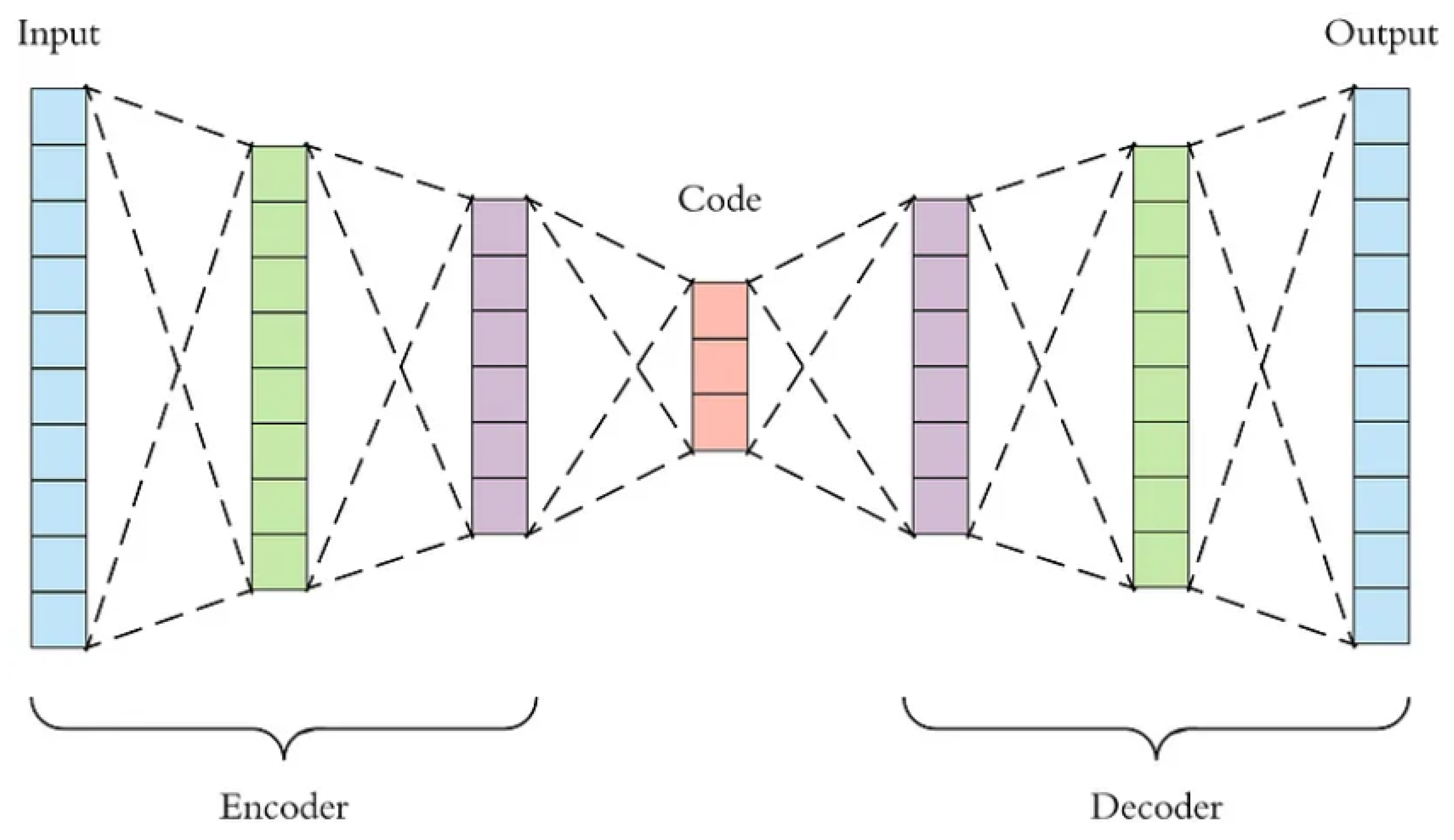
An autoencoder is a neural network architecture designed for unsupervised learning, consisting of an encoder and decoder. It aims to learn a compact representation of input data by reducing the reconstruction error between the original and reformed data. Figure 3 is an illustration of the autoencoder architecture.

Figure 1. Autoencoder architecture.

Figure 1. Autoencoder architecture.

$$x\stackrel{\mathrm{Encoder}}{⟶}h=e\left(x\right)\stackrel{\mathrm{Decoder}}{⟶}\widehat{x}=d\left(h\right)$$

The architecture of an autoencoder is designed to extract the hidden representation of input data through its encoder component. This representation, which exists in a reduced dimensional space, allows the model to discern non-linear characteristics of the input feature vector. In forecasting time series, these non-linear characteristics can offer valuable insights into the non-linear relationships among data points, which are crucial for forecasting future values. In the given equation, h signifies the hidden representation of the input data as obtained by the encoder component. The decoder component then reconstructs the data, denoted by $\widehat{x}$, by minimizing the reconstruction error. This process of reconstruction eliminates noise or outliers that are not correlated with the dataset, leaving behind only the significant features that are relevant to the context of the dataset. Autoencoders have proven to be effective tools for denoising across various fields [40,41].

3.2. Stacked AE-LSTM and AE-GRU Architecture

In the realm of financial time series forecasting, the process of extracting non-linear features from a dataset is of paramount importance. Financial time series data is unique in that it often exhibits non-linear characteristics. This means that the relationships between variables in the data are not simply proportional, but can change in complex ways. These non-linear relationships can be influenced by a multitude of factors, making them challenging to model accurately.

Algorithms designed for prediction tasks, such as those used in machine learning, are capable of learning from these inherent patterns within the data. They do this by adjusting their parameters to minimize the difference between their predictions and the actual data. Over time, this learning process allows the algorithm to improve its predictive accuracy. However, one of the challenges these algorithms face is the presence of outliers in the dataset. Outliers are data points that deviate significantly from the other observations. They could be the result of noise, errors, or genuinely exceptional observations. Regardless of their source, outliers can distort the learning process of the algorithm, leading it to make inaccurate predictions.

LSTM and GRU are commonly employed in the prediction of stocks and cryptocurrencies. However, these basic LSTM and GRU structures do not take into account the significance of non-linear features. In Natural Language Processing (NLP), both LSTM and GRU encounter difficulties in predicting words when the sentence length increases significantly. Consequently, these algorithms struggle to remember the context over a very long term. To address this issue, the Transformer Network (TN) was introduced, which uses an attention mechanism in an encoder-decoder architecture to remember the long-term context [42]. However, the encoder-decoder architecture of TN doesn’t compress the input vector for learning intricate features from the latent representation. The encoder component of the Transformer handles the processing of the input sequence, while the output sequence is produced by the decoder. However, the implementation of such a complex model is computationally demanding. In the prediction of financial time series, it is crucial to remember the long-term context of past significant market events. This aids in identifying similar trends and predicting future values based on these trends. Therefore, the basic LSTM and GRU architecture is not the optimal solution for this task. Typically, for a one-day-ahead forecast for stocks and cryptocurrencies, the training dataset is usually very large. Consequently, running such a large dataset with a TN architecture becomes computationally prohibitive. Encoder-decoder-based Recurrent Neural Network (RNN) architectures demonstrated effective performance when an Autoencoder-based LSTM was proposed [18]. To a certain degree, the encoded latent representation of the input data preserved the long-term contextual information about past observations, which helped to enhance the predictive accuracy of the basic LSTM architecture. This research found that significant improvements in predictive accuracy could be achieved through extensive experimentation with the model’s hyperparameters. However, in some studies, the GRU outperformed the LSTM in terms of achieving higher predictive accuracy. Therefore, this research also examines the accuracy of such an encoder-decoder architecture with GRU and proposes a new model with improvised performance.

In this paper, we introduce an innovative framework comprising stacked Autoencoder-based Long Short-Term Memory (AE-LSTM) and Gated Recurrent Unit (AE-GRU). The foundational structure of the proposed algorithm is elucidated in Figure 4. While both AE-LSTM and AE-GRU share a common architecture, distinct hyperparameters and activation functions tailored to each architecture were employed for optimal performance after strenuous investigation.

3.2.1. AE-LSTM

AE-LSTM, or Autoencoder-based LSTM, is a hybrid neural architecture that combines the capabilities of an autoencoder with LSTM units. Autoencoders are employed to learn a compressed representation of input data, and this encoded information is then fed into LSTM layers, enabling the model to capture and leverage long-term dependencies in sequential data. AE-LSTM is particularly effective in tasks involving time-series data, such as stock price prediction, where both feature learning and sequential context preservation are crucial for accurate forecasting. 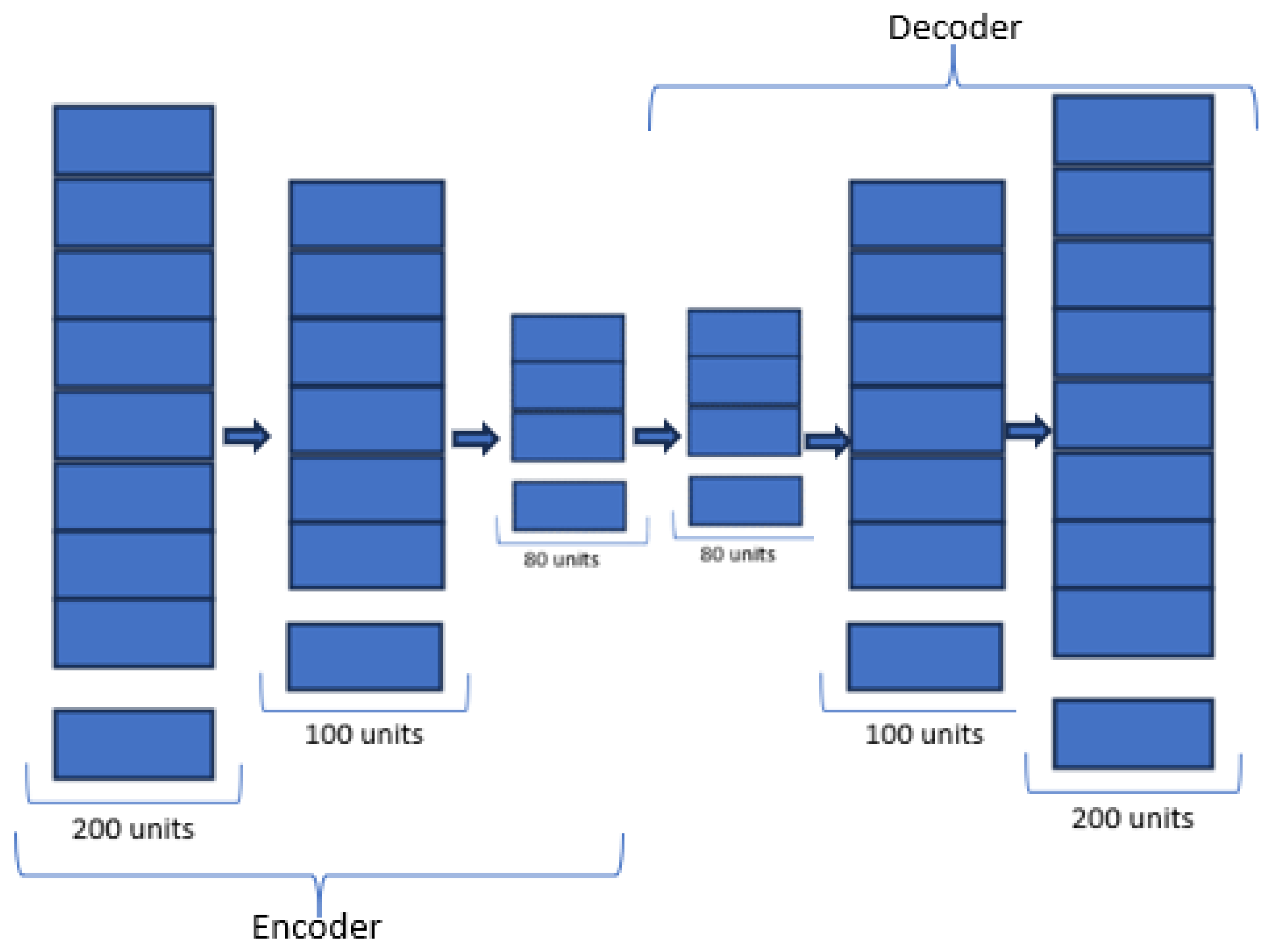Figure 2 represents the model structure of the proposed improvised AE-LSTM architecture.

$$\mathrm{Encoder}:x\stackrel{\mathrm{LSTM}200}{⟶}{h}_1\stackrel{\mathrm{LSTM}100}{⟶}{h}_2\stackrel{\mathrm{LSTM}80}{⟶}z$$

$$\mathrm{Decoder}:z\stackrel{\mathrm{LSTM}80}{⟶}{h}_3\stackrel{\mathrm{LSTM}100}{⟶}{h}_4\stackrel{\mathrm{LSTM}200}{⟶}\widehat{x}$$

In the given equation, it’s evident that the encoder structure employs several stacked LSTM layers to identify latent features at various compression levels. With each level of compression, the architecture learns more prominent features. However, additional compression leads to information loss. Such a deep architecture results in a higher reconstruction loss and is susceptible to the vanishing gradient problem. The initial compression occurs when the number of units in the second LSTM layer is reduced from 200 to 100. Over time, each layer experiences a reduction in units until the latent representation z is finally extracted from the LSTM layer with 80 units.

Similarly, the decoder layer incrementally increases the units in the subsequent LSTM layers. The entire structure is trained by minimizing the reconstruction loss. The output of the decoder is the reconstructed data that encapsulates the internal non-linear complexities of the financial time series. Ultimately, a Dense layer is employed to obtain the predicted output.

Figure 2. AE-based LSTM and GRU architecture.

Figure 2. AE-based LSTM and GRU architecture.

Algorithm 1 shows an algorithmic view of the proposed novel improvised encoder-decoder architecture of LSTM which outperforms the existing models.

Algorithm 1 AE-LSTM

1: $data\leftarrow parse("stock\_name")$  2: $normalized\_data\leftarrow normalize\left(data\right)$  3: $train\_data\leftarrow normalized\_data[start:end]$  4: $test\_data\leftarrow normalized\_data[start:end]$  5: $preprocessed\_train\leftarrow preprocess\left(train\right)$  6: $encoder\leftarrow LSTM(units=200,activation{=}^{\prime }activatio{n}^{\prime })(preprocessed\_train)$  7: $encoder\leftarrow LSTM(units=100,activation{=}^{\prime }activatio{n}^{\prime })\left(encoder\right)$  8: $encoder\leftarrow LSTM(units=80,activation{=}^{\prime }activatio{n}^{\prime })\left(encoder\right)$  9: $decoder\leftarrow LSTM(units=80,activation{=}^{\prime }activatio{n}^{\prime })\left(encoder\right)$  10: $decoder\leftarrow LSTM(units=100,activation{=}^{\prime }activatio{n}^{\prime })\left(decoder\right)$  11: $decoder\leftarrow LSTM(units=200,activation{=}^{\prime }activatio{n}^{\prime })\left(decoder\right)$  12: $model\leftarrow Model(encoder,decoder)$  13: $model.compile\left(\right)$  14: $predict\leftarrow model.predict(test\_data)$

3.2.2. AE-GRU

AE-GRU, or Autoencoder-Gated Recurrent Unit, is a hybrid neural network architecture that combines the capabilities of an autoencoder with a Gated Recurrent Unit (GRU). This innovative model integrates the feature learning abilities of autoencoders with the sequential modeling strengths of GRU, aiming to enhance the representation and prediction capabilities in various applications such as time series analysis and sequential data processing. The AE-GRU architecture involves the use of a stacked autoencoder for feature extraction, feeding the encoded features into GRU cells for capturing temporal dependencies and patterns. This combination leverages both unsupervised learning and recurrent neural network architectures to achieve improved performance in tasks requiring sequential data understanding and prediction. To our knowledge, this hybridization is a novel approach to financial asset price prediction. Figure 2 represents the model structure of the proposed novel AE-GRU algorithm.

$$\mathrm{Encoder}:x\stackrel{\mathrm{GRU}200}{⟶}{h}_1\stackrel{\mathrm{GRU}100}{⟶}{h}_2\stackrel{\mathrm{GRU}80}{⟶}z$$

$$\mathrm{Decoder}:z\stackrel{\mathrm{GRU}80}{⟶}{h}_3\stackrel{\mathrm{GRU}100}{⟶}{h}_4\stackrel{\mathrm{GRU}200}{⟶}\widehat{x}$$

In a manner akin to AE-LSTM, AE-GRU follows a similar architecture. Multiple encoder layers are layered to condense the feature vector into a representation in the latent space. After compressing to a feature vector, z, with an GRU layer consisting of 80 units, it is observed that further compression leads to a loss of information.

Several GRU layers, each with varying units, are stacked in a descending order to construct the encoder component of the AE-GRU architecture. This compression into the latent space z preserves valuable non-linear features of the financial time series. This latent feature vector encapsulates the long-term context derived from past observations.

Similarly, the decoder component incrementally increases the units in the GRU layers, resulting in an accurate reconstruction of the input data. This process eliminates outliers and extracts the non-linear contextual features from the financial data. Subsequently, a dense layer comprising a single unit is employed to predict future values.

Algorithm 2 shows an algorithmic view of the proposed novel encoder-decoder architecture of GRU, which outperforms the existing models and even the improvised AE-LSTM designed in this study. This encoder-decoder-based GRU architecture is novel and tested rigorously under varying market conditions. This proposed novel model overperforms existing architectures by retaining long-term non-linear contextual features.

Algorithm 2 AE-GRU

1: $data\leftarrow parse("stock\_name")$  2: $normalized\_data\leftarrow normalize\left(data\right)$  3: $train\_data\leftarrow normalized\_data[start:end]$  4: $test\_data\leftarrow normalized\_data[start:end]$  5: $preprocessed\_train\leftarrow preprocess\left(train\right)$  6: $encoder\leftarrow GRU(units=200,activation{=}^{\prime }activatio{n}^{\prime })(preprocessed\_train)$  7: $encoder\leftarrow GRU(units=100,activation{=}^{\prime }activatio{n}^{\prime })\left(encoder\right)$  8: $encoder\leftarrow GRU(units=80,activation{=}^{\prime }activatio{n}^{\prime })\left(encoder\right)$  9: $decoder\leftarrow GRU(units=80,activation{=}^{\prime }activatio{n}^{\prime })\left(encoder\right)$  10: $decoder\leftarrow GRU(units=100,activation{=}^{\prime }activatio{n}^{\prime })\left(decoder\right)$  11: $decoder\leftarrow GRU(units=200,activation{=}^{\prime }activatio{n}^{\prime })\left(decoder\right)$  12: $model\leftarrow Model(encoder,decoder)$  13: $model.compile\left(\right)$  14: $predict\leftarrow model.predict(test\_data)$

3.2.3. Hyperparameter Consideration

The process of tuning hyperparameters is a critical step in the development of machine learning or deep learning algorithms. Hyperparameters are distinct from other parameters in that their values are determined before the learning process begins. These are not derived from the data during training but are manually set to guide the learning process. The selection of these hyperparameters significantly influences the functioning of the algorithm. Incorrect choices could lead to sub-optimal performance, even for a model with high potential.

In this study, the Adam optimizer was chosen due to its widespread use in adaptively adjusting the learning rate while taking momentum into account. The first and second-moment exponential decay rates, represented by ${\beta }_1$ and ${\beta }_2$, were identified as the primary hyperparameters in this research. Additionally, this study explored three major activation functions to select the most suitable ones to improve the performance of the models. Other than that, rigorous investigation has been conducted to select the number of layers for designing the novel architecture.

Also upon considering multiple time windows, this research has decided to use 120 days past observation for predicting the one-day ahead forecast for stocks, cryptocurrencies, and stock index.

3.3. Activation Functions

This study examined three primary activation functions suitable for integration into the proposed hybridized models, namely: (1) Rectified Linear Unit (ReLU), (2) Exponential Linear Unit (ELU), and (3) Hyperbolic Tangent Function (tanh). These three activation functions are mostly used with DL architectures. The choice of activation function depends on the dataset and model architectures. Improper choice might result in sub-optimal performance.

Figure 3. Exponential Linear Unit.

Figure 3. Exponential Linear Unit.

3.3.1. ReLU

The Rectified Linear Unit (ReLU) activation function is extensively utilized in neural networks, providing non-linearity by outputting the input directly for positive values and zero for negative ones. Its popularity stems from its simplicity, computational efficiency, and effectiveness in dealing with the vanishing gradient problem during deep neural network training. ReLU addresses the issue of vanishing gradients that arise due to the saturation of neurons when sigmoid functions are used. Improper weight initialization can lead to the "dying ReLU" problem, especially due to the negative saturation.

The formula for ReLU is:

$$f_{Relu}\left(h_{i,k}\right)=max(0,h_{i,k}).$$

Figure 5(a) presents a graphical representation of ReLU1.

3.3.2. ELU

The Exponential Linear Unit (ELU) is an activation function commonly used in artificial neural networks. It brings non-linearity to the network by permitting the inclusion of negative values, unlike traditional activation functions such as ReLU. ELU has a smooth curve for negative inputs, avoiding the issue of dead neurons and enabling better convergence during training. It exhibits the ability to capture information from both positive and negative input ranges, contributing to improved learning in deep neural networks. ELU addresses the issue of the "dying ReLU" problem that occurs due to negative saturation but bad initialization still can cause underperformance. The ELU activation function is defined as: f(k)$=\left\{\begin{array}{cc}k\hfill & \mathrm{if}k>0\hfill \\ \alpha ·(e^k-1)\hfill & \mathrm{if}k\le 0\hfill \end{array}\right.$, where $\alpha$ is a positive hyperparameter controlling the slope of the function for negative inputs. Figure 5(b) presents a graphical representation of ELU 2.

3.3.3. Tanh

The hyperbolic tangent function, often denoted as $tanh\left(x\right)$, is a common activation function in neural networks. It squashes input values to the range of $(-1,1)$, making it zero-centered and aiding in mitigating vanishing gradient problems during training. The tanh activation is particularly useful in scenarios where zero-centered outputs are desired and has applications in various layers of neural network architectures. The tanh activation function delivers output centered around zero, but it can lead to the vanishing gradient problem due to neuron saturation caused by improper weight initialization. The formula for the tanh activation function:

$$tanh\left(k\right)=\frac{e^k-e^{-k}}{e^k+e^{-k}}$$

Figure 5(c) presents a graphical representation of tanh 3.

4. Experiments and Results

4.1. Dataset Consideration

The financial market encompasses a vast array of products derived from various sectors. Each financial product, whether it’s a derivative of stocks, cryptocurrencies, etc., reacts differently to distinct market events. Therefore, when developing a predictive model, it’s crucial to consider testing under a variety of market conditions with these diverse financial derivatives. In this study, three primary basic financial products are taken into account, from which multiple derivatives are formulated. These include volatile stocks from a range of sectors, the highly volatile cryptocurrency Bitcoin, and the moderately volatile yet stable stock index S&P. These are used for training and testing the proposed models.

To assess the effectiveness of our innovative Autoencoder-GRU and compare its performance with a hyperparameter-tuned Autoencoder-LSTM, this study has examined diverse stock datasets spanning various sectors. These include Apple (AAPL) (technology sector), Johnson and Johnson (JNJ) (healthcare sector), Chevron (CVX) (energy sector), JP Morgan Chase Bank (JPM) (banking sector), Bitcoin (BTC-USD) (cryptocurrency), and the S&P stock index (ĜSPC). The models were trained on data from 1998 to 2022, and their predictive capabilities were evaluated using data from 2023. Additionally, for Bitcoin, the training dataset spans from 2014 to 2022, with the model tested on data from 2023. The dataset analyzed includes significant market occurrences, including the 2001 dot-com bubble burst, the 2008 global financial crisis, and the market crash induced by the COVID-19 pandemic in 2020.

The efficiency of our proposed architecture has been evaluated across multiple machines to analyze its performance under the influence of various machine configurations. These include (a) a Dell Latitude 5540 intel core i7-1355U, 1.70 GHz, with 10 Core(s) and 16GB RAM; (b) an ASUS VivoBook X515EA intel core i5-1135G7, 2.40 GHz, with 4 Core(s) and 16GB RAM; (c) DELL Inc. OptiPlex 7040, intel core i5-6600, 3.30 GHz, with 4 core(s) and 16 GB RAM.

All these machines run Windows 11 OS and Jupiter Notebook as the IDE.

4.2. Exploratory Data Analysis

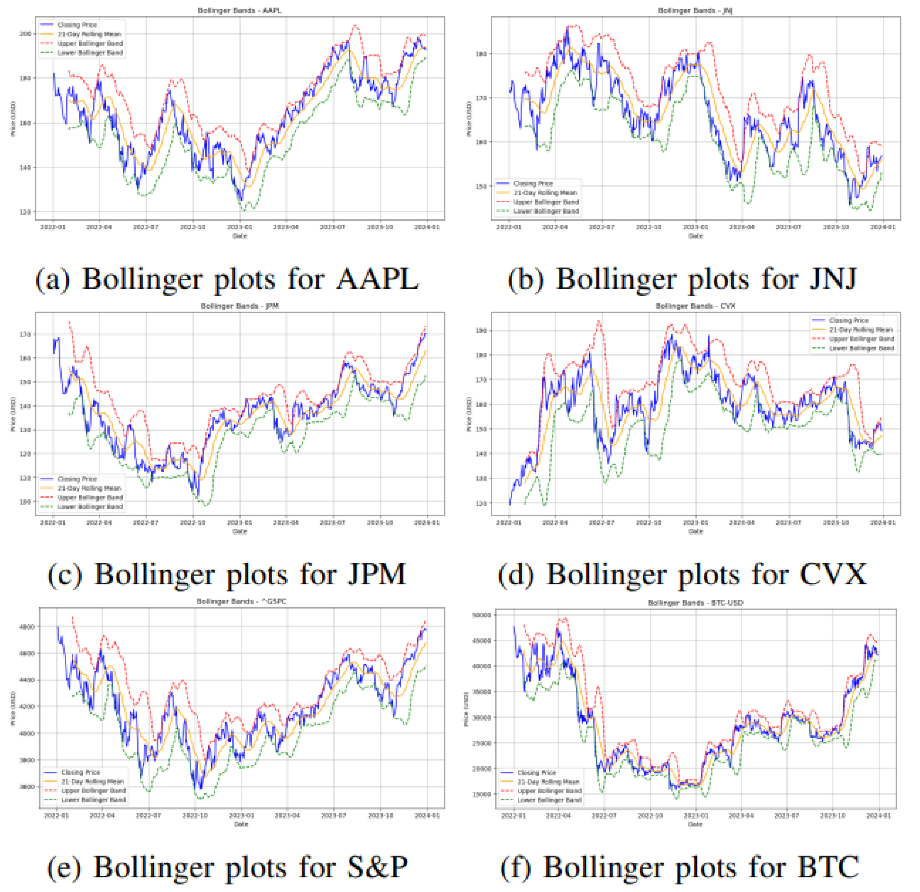
Figure 4 depicts the Bollinger bands for the financial instruments analyzed in this study. Both Figure 4 and Table 1 collectively indicate that AAPL and JPM display elevated volatility, while JNJ demonstrates comparatively lower volatility, and CVX exhibits a moderate level of volatility. S&P registers notably low average volatility, whereas the cryptocurrency bitcoin experiences the highest volatility between 2022 and 2023 among all the assets considered.

Figure 4. Bollinger plots for financial assets from 2022 to 2023.

Figure 4. Bollinger plots for financial assets from 2022 to 2023.

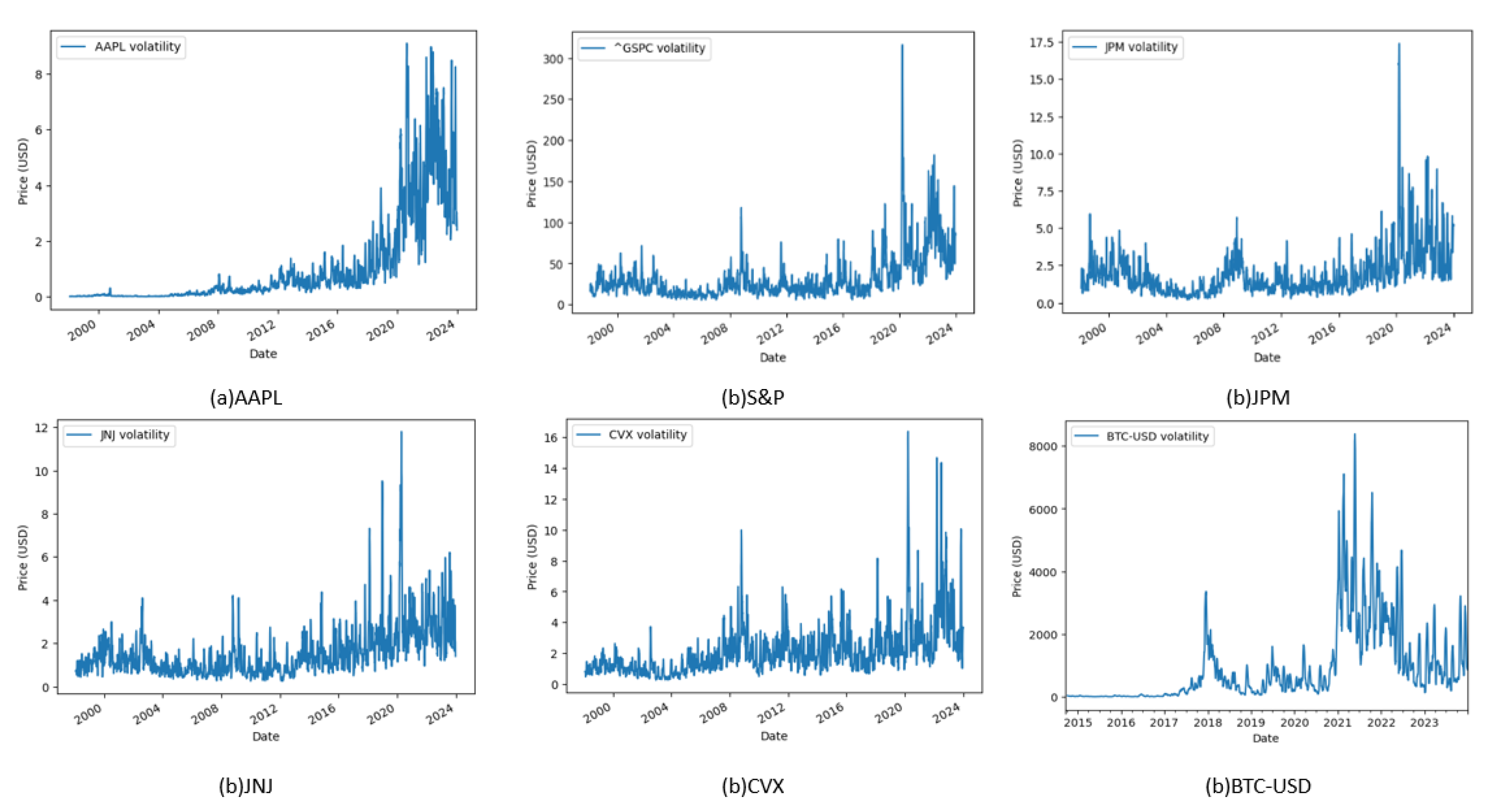
Figure 5 illustrates the change in the volatility trend in the considered timeframe. Notably, Apple stock exhibits a significant rise in volatility. Conversely, Bitcoin’s volatility displays abrupt fluctuations. The S&P, reflecting a blend of diverse financial assets, exhibits a high magnitude of volatility but lower average volatility. On the other hand, JPM, JNJ, and CVX consistently experience growth in volatility throughout the years.

Figure 5. Change in volatility.

Figure 5. Change in volatility.

4.3. Evaluation Metrics

In this research, the effectiveness of the model is assessed from five distinct viewpoints using five different evaluation metrics. Each of these metrics provides a unique way to test the model.

4.3.1. Mean Squared Error (MSE)

It serves as a commonly employed metric for regression analysis, evaluating the average squared disparity between predicted and actual values. This metric effectively gauges the variability or dispersion of these differences, imposing greater penalties for larger errors.

$$\mathrm{MSE}=\frac{1}{N}\sum _{i=1}^N{(a_i-{\widehat{a}}_i)}^2$$

Here $a_i$ is actual and ${\widehat{a}}_i$ is the forecast. N is the dataset size.

4.3.2. Root Mean Squared Error (RMSE)

It serves as a performance metric in regression analysis, measuring the mean measure of discrepancies between forecasted and true values. More precisely, it is derived from computing the square root of the MSE.

$$\mathrm{RMSE}=\sqrt{\mathrm{MSE}}$$

4.3.3. Mean Absolute Error (MAE)

It serves as a regression measure, quantifying the mean absolute discrepancy between forecasted and true values. This evaluation metric offers a straightforward evaluation of the model’s effectivity, assigning equal significance to each prediction error.

$$\mathrm{MAE}=\frac{1}{N}\sum _{i=1}^N|y_i-{\widehat{y}}_i|$$

4.3.4. R-squared (R2) Score

It measures the percentage of variance in the target variable captured by the prediction variables in a regression-based algorithm. The calculation involves comparing the sum of squared differences between forecasted and true values to the sum of squared differences between true values and their mean. A higher R-squared score, approaching 1, signifies a superior model fit, suggesting that a larger portion of the target variable’s variance is captured by the model.

$$R^2=1-\frac{{\sum }_{i=1}^N{(a_i-{\widehat{a}}_i)}^2}{{\sum }_{i=1}^N{(a_i-\overline{a})}^2}$$

Here $a_i$ is actual and ${\widehat{a}}_i$ is the forecast. N is the dataset size. $\overline{a}$ is the mean of the real values.

4.3.5. Mean Absolute Percentage Error (MAPE)

It quantifies the mean percent disparity between estimation and true values, offering a metric of the model’s effectiveness. A reduced MAPE signifies a closer match between predictions and real outcomes, rendering it an efficient metric for evaluating predictive precision across various industries. The formula for MAPE is given below:

$$MAPE=\frac{1}{n}\sum _n\left|\frac{\mathrm{actual}-\mathrm{prediction}}{\mathrm{actual}}\right|\times 100$$

4.4. Predictions by AE-LSTM vs AE-GRU

This research has considered three major activation functions—ReLU, tanh, and ELU. Other hyperparameters include 1st-moment exponential decay rate ${\beta }_1$, 2nd-moment exponential decay rate ${\beta }_2$, learning rate, and numerical stability. The models take 120 previous time-step data to predict the next step.

4.4.1. Predictions for Individual Stock

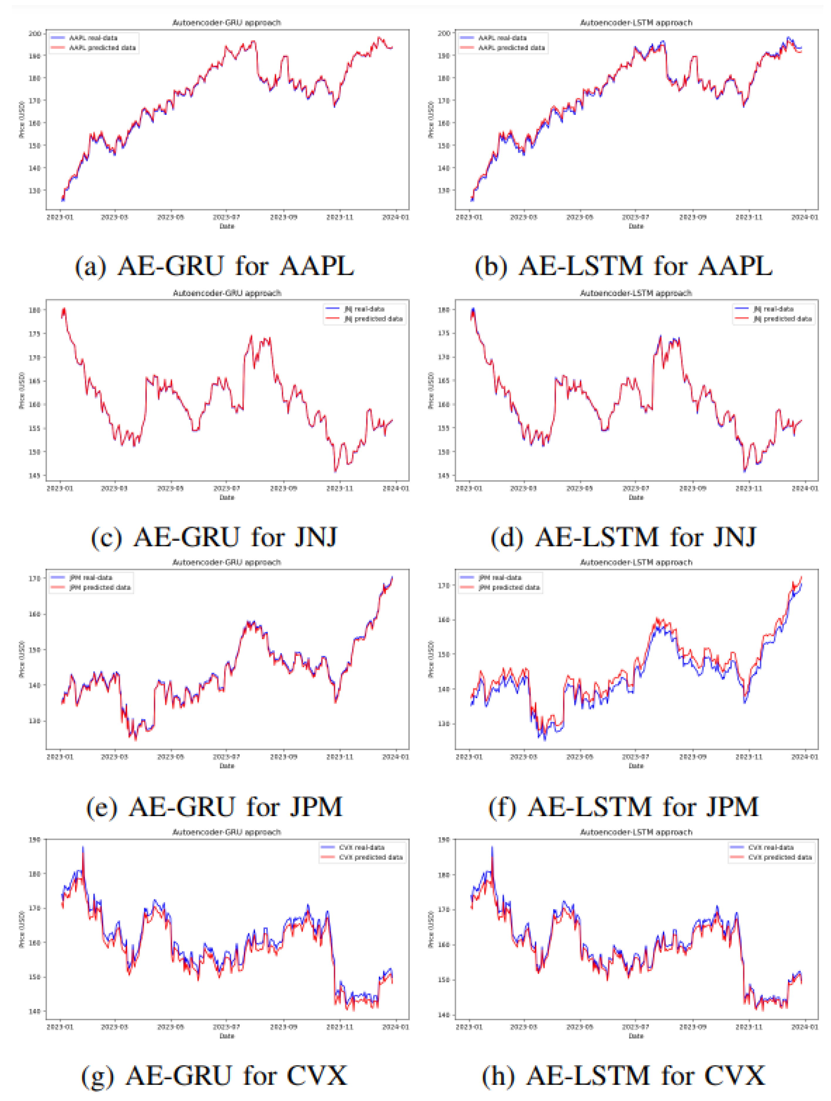
The suggested architecture of AE-GRU, employing ReLU as the activation function, outperforms AE-LSTM in the context of stocks AAPL, JNJ, JPM, and CVX. The extensive experimentation encompassed three activation functions and adjustments to hyperparameters, including 1st-moment exponential decay rate ${\beta }_1$, 2nd-moment exponential decay rate ${\beta }_2$, learning rate, and numerical stability set at $1\times {10}^{-7}$. Among various configurations of AE-LSTM, the setup with 1st-moment exponential decay rate, ${\beta }_1$ at 0.9, 2nd-moment exponential decay rate ${\beta }_2$ at 0.999, learning rate as 0.001, numerical stability at $1\times {10}^{-7}$, and ELU as the activation function proves to be the most effective. However, consistently, the proposed AE-GRU architecture with ReLU as the activation function outperforms AE-LSTM in these assessments. Figure 6 visually demonstrates the superiority in providing an accurate prediction of stock trends by AE-GRU compared to AE-LSTM-based predictions. Furthermore, Table 2 provides evidence that the superiority of AE-GRU over AE-LSTM is affirmed by five evaluation metrics.

4.4.2. Predictions for the Stock Index- S&P

Hyperparameter tuning for AE-GRU involves adjusting key parameters, such as setting 1st-moment and 2nd-moment exponential decay rates ${\beta }_1$ and ${\beta }_2$ to 0.9 and 0.999 respectively, the learning rate to 0.001, and maintaining numerical stability at $1\times {10}^{-7}$. Specifically for stock indices like S&P, AE-GRU performs optimally when using tanh as the activation function. In contrast, AE-LSTM with a ReLU activation function exhibits favorable outcomes compared to its other variants. 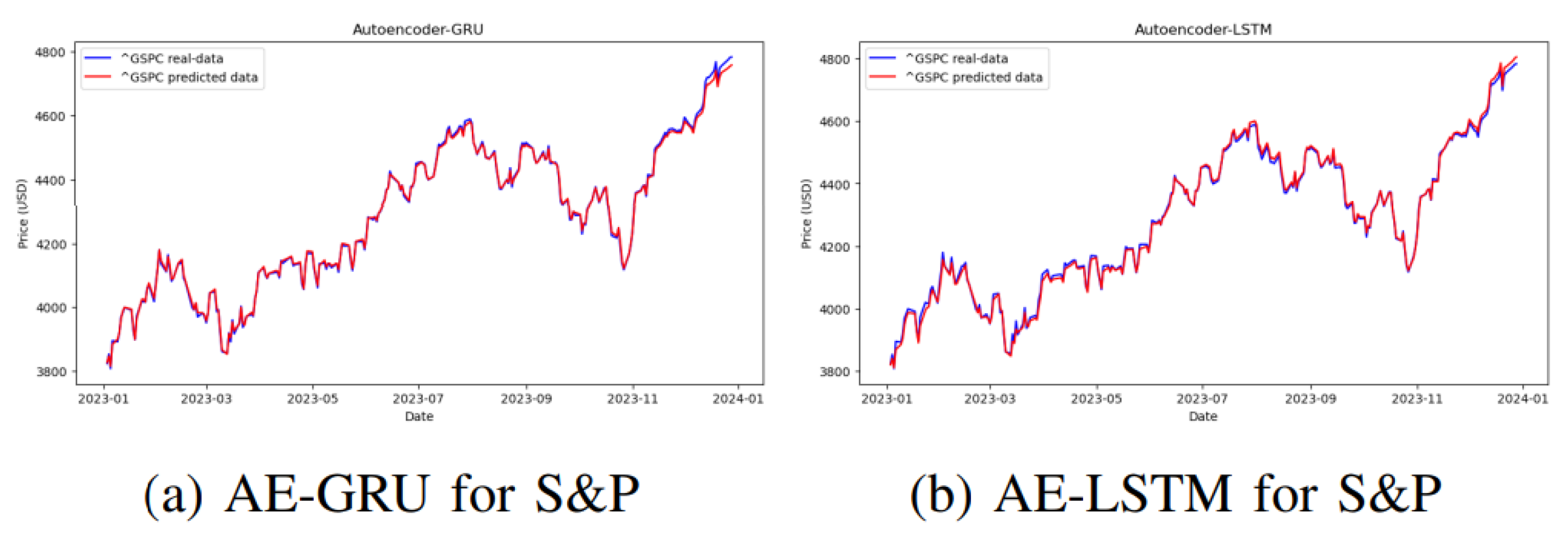However, in direct comparison, the tanh-based AE-GRU outperforms all variations of AE-LSTM in forecasting annual prices of S&P, as depicted in Figure 7. Despite a slightly higher MSE attributed to the large scale of values, the proposed AE-GRU architecture significantly outperforms AE-LSTM with an impressively low MAPE of 0.1%. Consequently, for stock index prediction, the proposed AE-GRU-based architecture demonstrates superiority over AE-LSTM which is illustrated in Figure 7.

4.4.3. Predictions for the Cryptocurrency- Bitcoin

Figure 8 demonstrates that the proposed AE-GRU design, utilizing ReLU as the activation function, outperforms the AE-LSTM prediction. Although hyperparameter tuning, employing ELU as the activation function, enhanced the predictive accuracy of the AE-LSTM structure to some degree, it still fell short of surpassing the novel AE-GRU design. The proposed AE-GRU architecture exhibited superior performance to the AE-LSTM architecture, achieving a MAPE of 0.5%, which is half the value observed in AE-LSTM.

5. Conclusions

The proposed architecture, AE-GRU, offers an innovative approach by combining encoder-decoder architecture and GRU, demonstrating superior performance compared to the existing AE-LSTM across various market scenarios. Experiments were conducted using stocks from different sectors and also included- S&P as the stock index, and bitcoin as a cryptocurrency. Across all sectors, the new deep learning model, AE-GRU, consistently outperformed the existing AE-LSTM. A novel AE-LSTM architecture is also designed in this study, which improvised the existing model through rigorous hyperparameter tuning. Despite experimenting with hyperparameter tuning for AE-LSTM and improvising its performance from the existing version, it still couldn’t match the prediction accuracy of the proposed novel AE-GRU architecture. Experiments were organized on three different computing devices, yielding similar results with slight variations in the values of evaluation metrics due to randomized weight initialization. The research considered data from significant market events of the 2001 high-tech bubble burst, the 2008 global financial crisis, and the 2020 COVID-19 stock market crisis. Our findings advocate for the adoption of the novel AE-GRU architecture, showcasing enhanced predictive accuracy for financial assets across various sectors and market conditions. The proposed encoder-decoder-based GRU architecture retains the long-term non-linear contexts from the past temporal observations resulting in superior efficacy in predicting future values for stocks, indexes, and highly volatile cryptocurrencies. After significant enhancements were made to the AE-LSTM architecture, the newly proposed AE-GRU architecture demonstrated superior performance. This research proposes an improvised and redefined version of AE-LSTM architecture along with novel AE-GRU architecture that provides higher predictive accuracy than the existing models.

6. Future Works

This research observes substantial efficacy after using an encoder-decoder-based architecture with RNN algorithms. Moreover, the proposed model takes much less time to train than the TN architectures with a similar amount of data. TN architectures also utilize encoder-decoder architecture but with multi-head attention. They don’t learn from the compressed latent representation from the input vectors. Further research can conduct a comparative analysis between the TN and the proposed architectures by extensive investigation. Moreover, the proposed model could be made more robust by adding learnable filters to conduct more specific feature extraction. Other than that, context retention in the model through a model-agnostic vectorized representation of the data before feeding into the model could be an interesting addition to the presently proposed research. Also, ML algorithms are generally sensitive to a lot of parameters. Our purpose in this study was to hyperparameter tune the model in such a way that the proposed novel AE-GRU shows less variation under various circumstances. In our further research endeavor we aim to extend our investigation to conduct detailed sensitivity analysis of different parameters under various market conditions. Sensitivity analysis could certainly be a new focus of research. To address machine dependencies, thorough hyperparameter tuning is recommended controlling features like weight optimization, necessitating experimentation with high-performance computing. which we plan to consider in the future.

Appendix A.1. LSTM

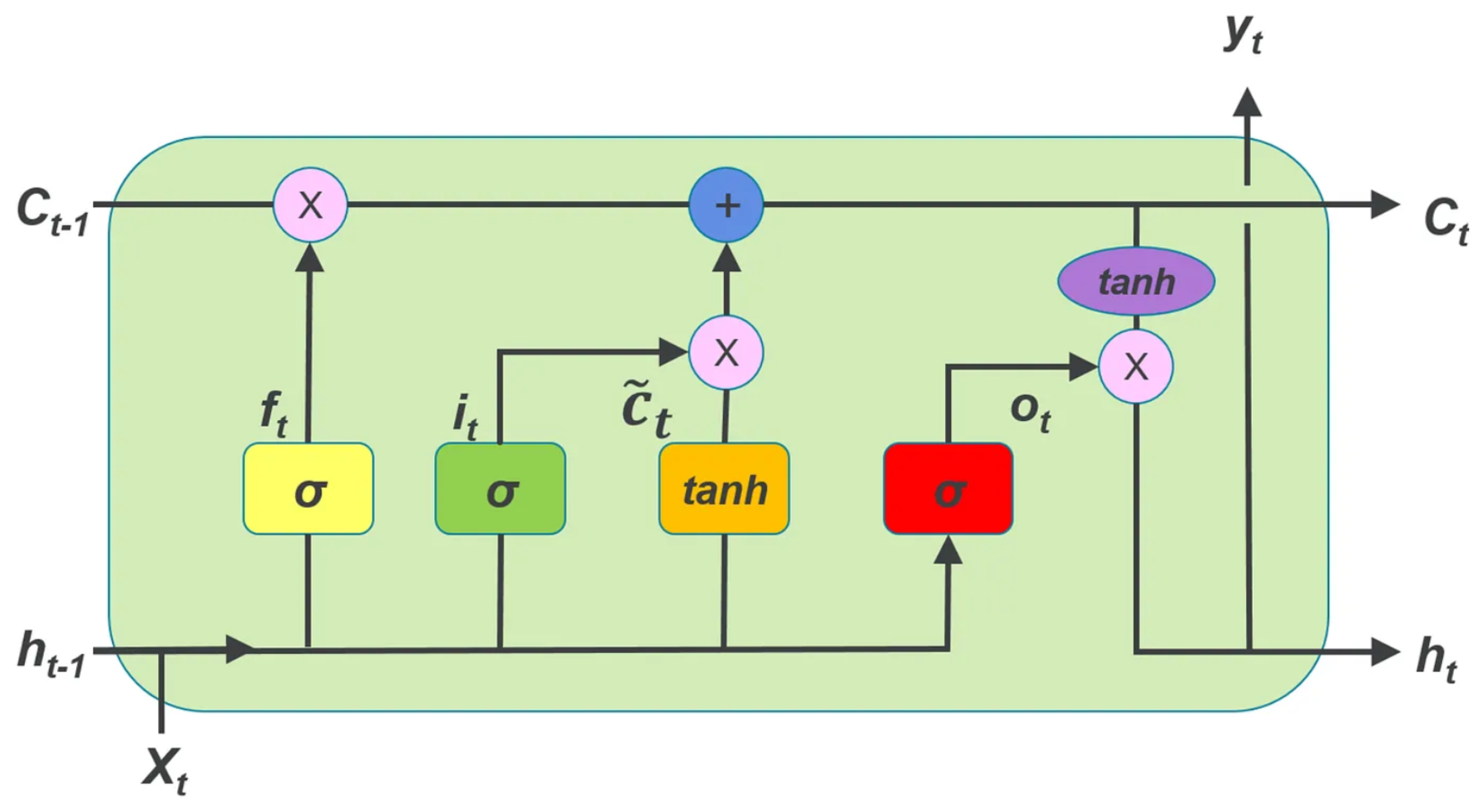
LSTM is an RNN architecture that can handle long-term dependencies in the data [43] address the issue of vanishing gradient faced by the basic RNN. From Figure 1, we can see that it comprises specialized memory units that can maintain and update information over extended sequences4. These memory units, called cells, contain three gating mechanisms: input, output, and forget gates. The input gate oversees the selection of data to be stored in the cell, the forget gate governs the determination of information to be discarded, and the output gate manages the information to be emitted from the cell.

Figure A1. LSTM architecture.

Figure A1. LSTM architecture.

The LSTM equations:

$$\begin{array}{cc}\hfill f_t& =\sigma (W_f·[h_{t-1},x_t]+b_f)\hfill \\ \hfill i_t& =\sigma (W_i·[h_{t-1},x_t]+b_i)\hfill \\ \hfill {\tilde{C}}_t& =tanh(W_C·[h_{t-1},x_t]+b_C)\hfill \\ \hfill C_t& =f_t\odot C_{t-1}+i_t\odot {\tilde{C}}_t\hfill \\ \hfill o_t& =\sigma (W_o·[h_{t-1},x_t]+b_o)\hfill \\ \hfill h_t& =o_t\odot tanh\left(C_t\right)\hfill \end{array}$$

${\mathrm{f}}_t$ is the forget gate, governing the information to be omitted from the cell state. ${\mathrm{i}}_t$ denotes the input gate, deciding which values to revise in the cell state. ${\tilde{\mathrm{C}}}_t$ signifies the candidate cell state, presenting new candidate values for the cell state. ${\mathrm{C}}_t$ represents the cell state, storing long-term information. ${\mathrm{o}}_t$ indicates the output gate, managing the information for output from the cell state. ${\mathrm{h}}_t$ corresponds to the hidden state, encompassing the short-term information for output.

Appendix A.2. GRU

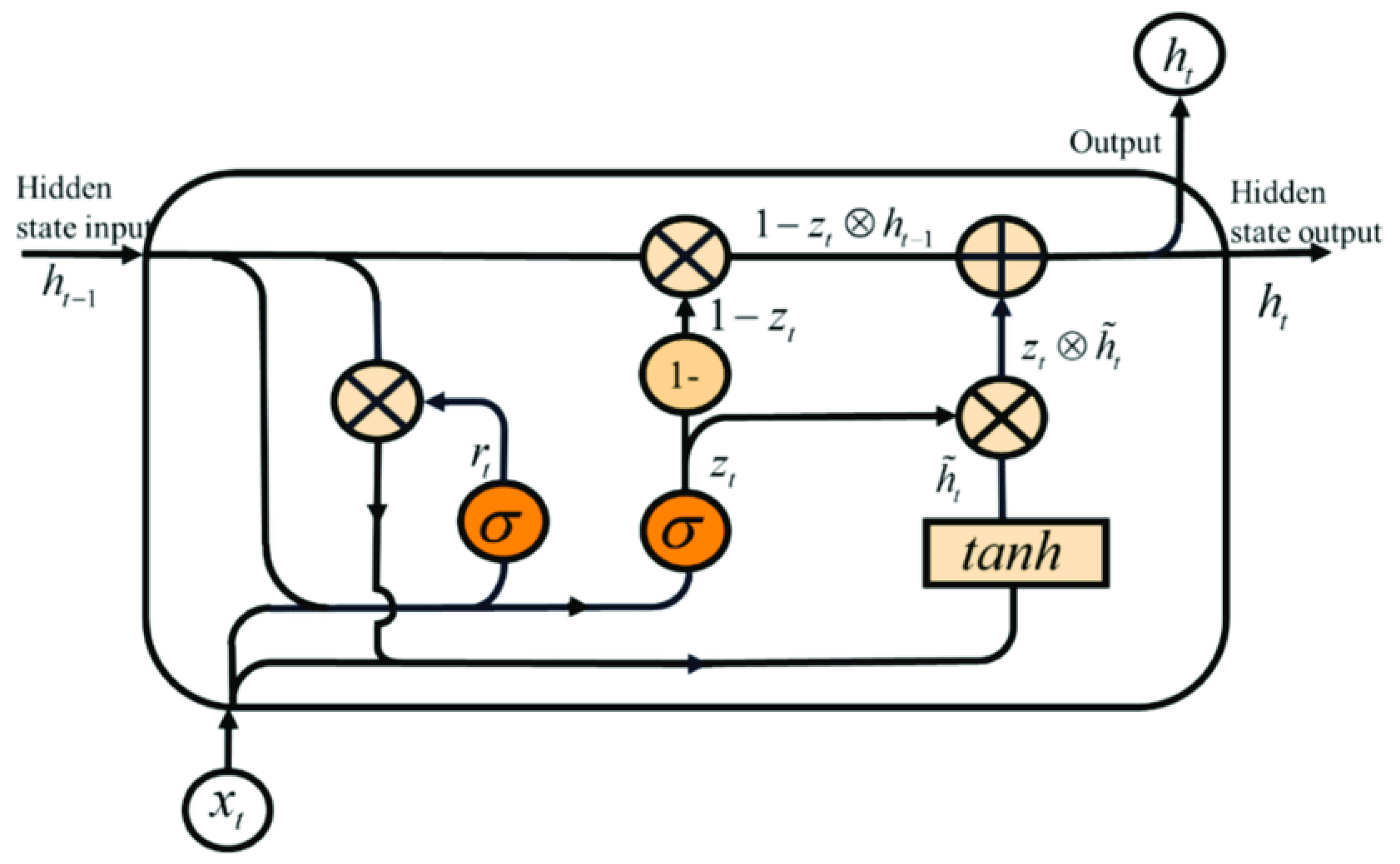
The GRU, a prevalent RNN algorithm in stock price prediction, exhibits a unique architecture with gating mechanisms regulating information flow, enhancing long-term dependency capture in input data5. Core components, including reset and update gates, enable effective context utilization as seen in Figure 2. GRU’s computational efficiency, attributed to its simpler two-gate structure, contributes to faster training times compared to LSTM [44].

Figure A2. GRU architecture

Figure A2. GRU architecture

The following equations can explain GRU:

$$\begin{array}{cc}\hfill r_t& =\sigma (W_r{x}_t+U_r{h}_{t-1})\hfill \\ \hfill z_t& =\sigma (W_z{x}_t+U_z{h}_{t-1})\hfill \\ \hfill {\tilde{h}}_t& =tanh(r_t\odot U{h}_{t-1}+W{x}_t)\hfill \\ \hfill h_t& =(1-z_t)\odot {\tilde{h}}_t+z_t\odot h_{t-1}\hfill \end{array}$$

In the context of the GRU model, $r_t$ serves as the reset gate, while $z_t$ functions as the update gate. The vector ${\tilde{h}}_t$ represents a candidate activation vector. The functions $\sigma$ and tanh denote the sigmoid and hyperbolic tangent functions, respectively. The weight matrices $W_r$, $U_r$, $W_z$, $U_z$, W, and U play pivotal roles in the model.

LSTMs employ a more intricate structure with separate gates for input, forget, and output, enabling them to preserve long-term dependencies in the input sequence by controlling the flow of information. In contrast, GRUs feature a simplified architecture by merging the functionality of the input and forget gates into a single "update gate," resulting in fewer parameters and computational resources. While LSTMs maintain separate cell states and hidden states for memory management, GRUs combine them into a single vector, which may slightly reduce memory capacity. Both LSTM and GRU units have demonstrated effectiveness in various applications, and the choice between them often depends on factors such as model complexity and computational resources.

References

- Metghalchi, M.; Marcucci, J.; Chang, Y.H. Are moving average trading rules profitable? Evidence from the European stock markets. Applied Economics 2012, 44, 1539–1559. [CrossRef]
- Banerjee, D. Forecasting of Indian stock market using time-series ARIMA model. 2014 2nd international conference on business and information management (ICBIM). IEEE, 2014, pp. 131–135. [CrossRef]
- McMillan, D.G. Non-linear predictability of UK stock market returns. Oxford Bulletin of Economics and Statistics 2003, 65, 557–573. [CrossRef]
- Hiransha, M.; Gopalakrishnan, E.A.; Menon, V.K.; Soman, K. NSE stock market prediction using deep-learning models. Procedia computer science 2018, 132, 1351–1362. [CrossRef]
- Sirisha, U.M.; Belavagi, M.C.; Attigeri, G. Profit prediction using Arima, Sarima, and LSTM models in time series forecasting: A Comparison. IEEE Access 2022, 10, 124715–124727. [CrossRef]
- Kumbure, M.M.; Lohrmann, C.; Luukka, P.; Porras, J. Machine learning techniques and data for stock market forecasting: A literature review. Expert Systems with Applications 2022, 197, 116659. [CrossRef]
- Cakra, Y.E.; Distiawan Trisedya, B. Stock price prediction using linear regression based on sentiment analysis. 2015 International Conference on Advanced Computer Science and Information Systems (ICACSIS), 2015, pp. 147–154. [CrossRef]
- Lawal, Z.K.; Yassin, H.; Zakari, R.Y. Stock market prediction using supervised machine learning techniques: An overview. 2020 IEEE Asia-Pacific Conference on Computer Science and Data Engineering (CSDE). IEEE, 2020, pp. 1–6. [CrossRef]
- Hindrayani, K.M.; Fahrudin, T.M.; Aji, R.P.; Safitri, E.M. Indonesian stock price prediction including covid19 era using decision tree regression. 2020 3rd International Seminar on Research of Information Technology and Intelligent Systems (ISRITI). IEEE, 2020, pp. 344–347. [CrossRef]
- Chen, J. Analysis of bitcoin price prediction using machine learning. Journal of Risk and Financial Management 2023, 16, 51. [CrossRef]
- Khedr, A.M.; Arif, I.; El-Bannany, M.; Alhashmi, S.M.; Sreedharan, M. Cryptocurrency price prediction using traditional statistical and machine-learning techniques: A survey. Intelligent Systems in Accounting, Finance and Management 2021, 28, 3–34. [CrossRef]
- Shahi, T.B.; Shrestha, A.; Neupane, A.; Guo, W. Stock price forecasting with deep learning: A comparative study. Mathematics 2020, 8, 1441. [CrossRef]
- Pintelas, E.; Livieris, I.E.; Stavroyiannis, S.; Kotsilieris, T.; Pintelas, P. Investigating the problem of cryptocurrency price prediction: a deep learning approach. Artificial Intelligence Applications and Innovations: 16th IFIP WG 12.5 International Conference, AIAI 2020, Neos Marmaras, Greece, June 5–7, 2020, Proceedings, Part II 16. Springer, 2020, pp. 99–110.
- Liou, C.Y.; Cheng, W.C.; Liou, J.W.; Liou, D.R. Autoencoder for words. Neurocomputing 2014, 139, 84–96. [CrossRef]
- Gu, S.; Kelly, B.; Xiu, D. Autoencoder asset pricing models. Journal of Econometrics 2021, 222, 429–450. [CrossRef]
- Xia, K.; Huang, J.; Wang, H. LSTM-CNN architecture for human activity recognition. IEEE Access 2020, 8, 56855–56866. [CrossRef]
- Pierre, A.A.; Akim, S.A.; Semenyo, A.K.; Babiga, B. Peak Electrical Energy Consumption Prediction by ARIMA, LSTM, GRU, ARIMA-LSTM and ARIMA-GRU Approaches. Energies 2023, 16, 4739. [CrossRef]
- Selby, N.; Taparia, A.; others. An Efficient Stock Price Prediction Mechanism Using Multivariate Sequential LSTM Autoencoder 2023.
- Zhong, X.; Enke, D. Forecasting daily stock market return using dimensionality reduction. Expert Systems with Applications 2017, 67, 126–139. [CrossRef]
- Kohli, P.; Zargar, S.; Arora, S.; Gupta, P. Stock Prediction Using Machine Learning Algorithms. Applications of Artificial Intelligence Techniques in Engineering. Springer, Singapore, 2019, pp. 1–38. [CrossRef]
- Hu, Z.; Zhao, Y.; Khushi, M. A Survey of Forex and Stock Price Prediction Using Deep Learning. Applied System Innovation 2021, 4, 9. [CrossRef]
- Jiang, W. Applications of deep learning in stock market prediction: Recent progress. Expert Systems with Applications 2021, 184, 115537. [CrossRef]
- Nikou, M.; Mansourfar, G.; Bagherzadeh, J. Stock Price Prediction using Deep Learning Algorithm and its Comparison with Machine Learning Algorithms. Intelligent Systems in Accounting, Finance and Management 2019, 26, 164–174. [CrossRef]
- Sheth, D.; Shah, M. Predicting Stock Market Using Machine Learning: Best and Accurate Way to Know Future Stock Prices. International Journal of Systems Assurance Engineering and Management 2023, 14, 1–18. [CrossRef]
- Ali, M.; Khan, D.M.; Alshanbari, H.M.; El-Bagoury, A.A.H. Prediction of Complex Stock Market Data Using an Improved Hybrid EMD-LSTM Model. Applied Sciences 2023, 13, 1429. [CrossRef]
- Qi, C.; Ren, J.; Su, J. GRU Neural Network Based on CEEMDAN–Wavelet for Stock Price Prediction. Applied Sciences 2023, 13, 7104. [CrossRef]
- Karmiani, D.; Kazi, R.; Nambisan, A.; Shah, A.; Kamble, V. Comparison of Predictive Algorithms: Backpropagation, SVM, LSTM and Kalman Filter for Stock Market. 2019 Amity International Conference on Artificial Intelligence (AICAI), 2019, pp. 228–234. [CrossRef]
- Jiang, Q.; Tang, C.; Chen, C.; Wang, X.; Huang, Q. Stock Price Forecast Based on LSTM Neural Network. Proceedings of the Twelfth International Conference on Management Science and Engineering Management. ICMSEM 2018; Xu, J.; Cooke, F.; Gen, M.; Ahmed, S., Eds. Springer, 2019, pp. 403–412.
- Fang, Z.; Ma, X.; Pan, H.; Yang, G.; Arce, G.R. Movement Forecasting of Financial Time Series Based on Adaptive LSTM-BN Network. Expert Systems with Applications 2023, 213, 119207. [CrossRef]
- Gupta, P.; Gao, Y.; Wang, R.; Zhou, E. Stock Prediction Based on Optimized LSTM and GRU Models. Scientific Programming 2021, p. 4055281. [CrossRef]
- Kim, J.; Kim, S.; Wimmer, H.; Liu, H. A cryptocurrency prediction model using LSTM and GRU algorithms. 2021 IEEE/ACIS 6th International Conference on Big Data, Cloud Computing, and Data Science (BCD). IEEE, 2021, pp. 37–44. [CrossRef]
- Gradxs, G.P.B.; Rao, D.N. Behaviour Based Credit Card Fraud Detection: Design and Analysis by Using Deep Stacked Autoencoder Based Harris Grey Wolf (HGW) Method. Scandinavian Journal of Information Systems 2023, 35, 1–8.
- Fanai, H.; Abbasimehr, H. A Novel Combined Approach Based on Deep Autoencoder and Deep Classifiers for Credit Card Fraud Detection. Expert Systems with Applications 2023, 217, 119562. [CrossRef]
- Zhao, H.; Li, X.; Xu, J.; Fu, X.; Chen, J. Financial Time Series Data Prediction by Combination Model Adaboost-KNN-LSTM. 2023 International Joint Conference on Neural Networks (IJCNN); IEEE: Gold Coast, Australia, 2023; pp. 1–8. [CrossRef]
- Kwak, N.; Lim, D. Financial Time Series Forecasting using AdaBoost-GRU Ensemble Model. Journal of the Korean Data And Information Science Society 2021, 32, 267–281. [CrossRef]
- Shen, G.; Tan, Q.; Zhang, H.; Zeng, P.; Xu, J. Deep Learning with Gated Recurrent Unit Networks for Financial Sequence Predictions. Procedia Computer Science 2018, 131, 895–903. [CrossRef]
- Hossain, M.A.; Karim, R.; Thulasiram, R.; Bruce, N.D.B.; Wang, Y. Hybrid Deep Learning Model for Stock Price Prediction. Proc. 2018 IEEE Symposium on Computational Intelligence in Financial Engineering and Economics (CIFEr), Symposium Series on Computational Intelligence; IEEE: Bangalore, India, 2018. [CrossRef]
- Song, H.; Choi, H. Forecasting Stock Market Indices Using Recurrent Neural Network Based Hybrid Models: CNN-LSTM, GRU-CNN, and Ensemble Models. Applied Sciences 2023, 13, 4644. [CrossRef]
- Petrovic, A.; Strumberger, I.; Bezdan, T.; Jassim, H.S.; Nassor, S.S. Cryptocurrency price prediction by using hybrid machine learning and beetle antennae search approach. 2021 29th Telecommunications Forum (TELFOR). IEEE, 2021, pp. 1–4. [CrossRef]
- Lu, X.; Tsao, Y.; Matsuda, S.; Hori, C. Speech enhancement based on deep denoising autoencoder. Interspeech, 2013, Vol. 2013, pp. 436–440.
- Saad, O.M.; Chen, Y. Deep denoising autoencoder for seismic random noise attenuation. Geophysics 2020, 85, V367–V376. [CrossRef]
- Vaswani, A.; Shazeer, N.; Parmar, N.; Uszkoreit, J.; Jones, L.; Gomez, A.N.; Kaiser, .; Polosukhin, I. Attention is all you need. Advances in neural information processing systems 2017, 30.
- Graves, A.; Graves, A. Long short-term memory. Supervised sequence labelling with recurrent neural networks 2012, pp. 37–45.
- Yang, S.; Yu, X.; Zhou, Y. Lstm and gru neural network performance comparison study: Taking yelp review dataset as an example. 2020 International workshop on electronic communication and artificial intelligence (IWECAI). IEEE, 2020, pp. 98–101. [CrossRef]