Analysis of Behavioural Thermoregulatory Responses in Giraffa, Regarding Temperature and Sunlight Exposure during Daylight Hours

Preprint

Article

Analysis of Behavioural Thermoregulatory Responses in Giraffa, Regarding Temperature and Sunlight Exposure during Daylight Hours

Altmetrics

Downloads

119

Views

Comments

Supplementary Material

supplementary.xlsx (566.95KB )

Rowan Samuel Masterman^*

This version is not peer-reviewed

Submitted:

27 March 2024

Posted:

27 March 2024

You are already at the latest version

Alerts

Abstract

Research topics surrounding the giraffe have been subject to recent disagreement, with work focusing on taxonomy over ecological phenomena such as behavioural thermoregulation. Much interest in taxonomy arises around the existence of distinct local populations of giraffes, often enclosed in small, fenced reserves, preventing natural gene flow. Targeted management of reserves may act as a buffer for declining populations, providing landscape that minimises requirements for thermoregulatory behaviours. Notable behaviours include shade-usage via trees and other giraffes, and positioning of the body towards the sun, employing an individual’s own neck as a shade source. Breeding programmes and translocation of individuals away from large communities on fenced reserves may increase giraffe population numbers across their range; however, the genetic diversity of large populations in enclosed spaces may be called into question. 55 of the 57 giraffes from the population on the Mogalakwena River Reserve (MRR) were observed over eight months, recording thermoregulatory behaviours such as body positioning in response to sun exposure, and shade usage; behaviours both noted in secondary works. These behaviours were compared across identities, such as sex and age, to assess how thermoregulation varies per individual. The population on the MRR spent more time facing the sun during high temperature days, with adults, sub-adults, males, and dark-coated individuals prioritising the behaviour beyond other individuals. Body positioning behaviours of individuals were also found to be more important in thermoregulation than shade-seeking, with shade usage decreasing on hotter days. Positional behaviour, disregarding identity, was also observed across wet and dry seasons, with a clear contrast; giraffes face the sun significantly more during the hotter wet season. The behaviours observed in this work provide an insight into the direction conservational strategies may take on closed reserves. However, further work is required on other reserves with varied population structures, to determine whether one strategy may be implemented across the giraffe's range, or whether specialised strategies are required in individual locations.

Keywords:

Subject: Biology and Life Sciences - Ecology, Evolution, Behavior and Systematics

1. Introduction

Efforts into the conservation of giraffes, formerly ‘Giraffa camelopardalis’, have led to the potential restructuring of previously documented giraffe lineages. Upon initial classification, it was accepted that one giraffe species existed, divided into nine sub-species comprised of non-interbreeding populations [1]. However, recent research suggests that it is more appropriate to consider four genetically distinct major species of giraffes, with five potential sub-species in discrete locations across Africa [2,3]. This restructuring of the giraffe genus has led to some consternation regarding current giraffe vulnerability assessments. Recent reports on the IUCN red list [4] suggest that giraffes as a species should be classified as vulnerable due to extensive population decay, whereas Deacon and Tutchings [5] argue that populations of the major South African sub-species ‘Giraffa camelopardalis giraffa’ are stable and may be increasing.

Within the Mogalakwena Research Centre (MRC), the consensus is that research on giraffes should focus on ‘Giraffa giraffa giraffa’; a sub-species from one of four recently proposed major species. This sub-species is referred to as the South African giraffe, or Cape giraffe. The South African giraffe has a range covering: south-eastern Angola, northern Botswana, southern Mozambique, northern South Africa, south-western Zambia, and areas in Zimbabwe [6].

Thermoregulation, which comprises the body of this work, is defined generally as “the maintenance of a relatively constant core body temperature” [7]. Several different mechanisms of thermoregulation have been previously identified. The use of different sets of mechanisms is used to divide organisms into ‘ectotherms’ and ‘endotherms’ [8]. Ectotherms are defined as organisms that rely entirely on the external environment to maintain a stable internal temperature [9,10]. Endotherms, or warm-blooded animals, on the other hand, are defined as organisms that employ primarily metabolic heat production to maintain a stable internal temperature. Endothermy is a key characteristic of birds [11] and mammals [12], such as the giraffe.

According to Tan and Knight [13], studies on thermoregulation often split the body into two key components: the external surface, which fluctuates with temperature, and the core, which maintains a stable temperature. The internal core is the target of the thermoregulatory response system (Hensel 1973, cited in Tan and Knight [13], which employs the key components in two major ‘responses’, with a convergent goal of maintaining a set temperature.

Feedback responses are full-body responses which are enacted when core temperature undergoes a major fluctuation; These fluctuations are detected by thermoreceptors throughout the core of the body [14]. Feed-forward responses, on the other hand, are pre-emptive actions, undertaken when a perceived thermal challenge that does not affect the core arises; for example, cutaneous sensation of temperature changes may lead to a thermoregulatory reflex, minimising the effect of ambient environmental temperature [15].

In mammals, feedback and feed-forward responses can be separated into physiological and behavioural reflexes. Physiological reflexes consist of involuntary, primarily autonomic actions, which aim to generate or dissipate heat, opposing the external temperature [13]; Two examples of this are cutaneous vasodilation and reduced thermogenesis [16]. Behavioural reflexes, on the other hand, are goal-oriented actions, and are reinforced through attainment of rewards, such as relief from negative sensations attributed to hypo- or hyperthermia. The two most prominent behavioural reflexes are warm- and cold-seeking [17,18].

The giraffe, a large endothermic mammal, has been previously noted to have specialised body structures to aid physiological thermoregulation. These include a thin, long neck and legs, which aid in evaporative and convective heat loss, whilst maintaining a surface area to volume ratio that is characteristic of many mammals. In prior research [19], it was also ascertained that giraffes employ behavioural reflexes to combat extreme weathers observed across Africa. Two major behaviours aiming to reduce heat absorption have been observed: facing the sun during direct exposure, and shade-seeking. Facing the sun is hypothesised to be a method of employing the neck of the giraffe, casting shade over the main bulk of the body to reduce net absorption of solar radiation.

This study aimed to examine the observation that giraffes use their neck to cast shade over the body as a behavioural thermoregulatory response, considering the effects of sun exposure and temperature on a local population of giraffes.

Project aims will be broken down into individual hypotheses, which will seek to determine how behaviours and different identities are affected by temperature and exposure. The hypotheses tested are as follows:

Giraffes spend more time facing the sun as temperature increases.
Adult giraffes spend more time facing the sun as thermoregulatory behaviours may be learned.
Male giraffes are predicted to have darker coat colours, so will spend more time facing the sun.
Individuals with darker coats, of any sex, are expected to spend more time facing the sun, due to increased heat absorption.
Giraffes will use more shade as temperature increases, to combat increased rates of heat absorption.
Giraffes will spend more time facing the sun during wet season, compared to dry season, due to increased temperatures.

2. Materials and Methods

2.1. Study Area

The study was conducted on the Mogalakwena River Reserve (MRR; 22°43'23.6"S 28°47'19.4"E), which comprises a fenced area of 1,500 hectares, situated in the Limpopo province of South Africa [20] (Figure A1). The reserve is situated in the Savanna biome [21] and is characterised by plains interspersed with areas of shrubbery and woodland. The Savanna is split into bioregions, which can be divided by vegetation types [22]. The vegetation of the MRR is characterised as ’Arid Sweet Bushveld’ (Acocks 1952, cited in Mucina and Rutherford [21]), or ‘Sweet Bushveld’ (Low and Rebelo 1996, cited in Mucina and Rutherford [21]). This vegetation type consists of plains, short open woodland, and thickets of mainly Acacia erubescens, A. mellifera (blackthorn), and Dichrostachys cinerea (sickle bush [21]).

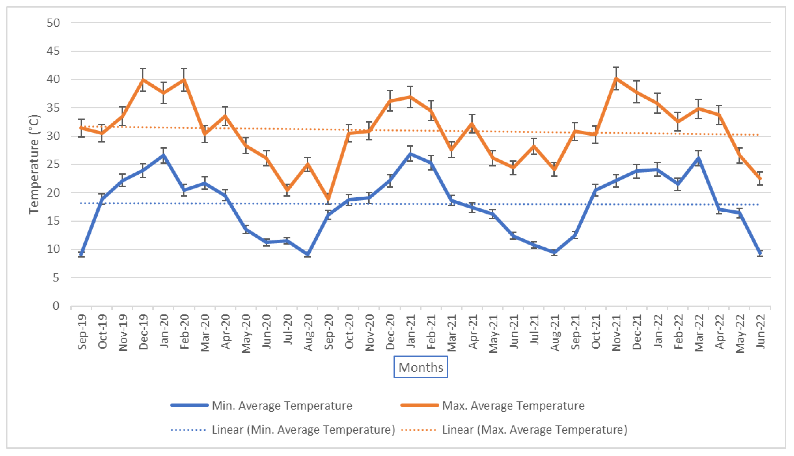
On the MRR, the maximum and minimum daily temperatures have been recorded since September 2019. This has allowed the observation of two major seasons: summer (wet season) and winter (dry season). The summer months of October to April 2020-21 consisted of an approximate average maximum temperature of 33°C, and a minimum of 21°C. This was a noticeable contrast to the winter months of May to September 2020-21, where an average maximum temperature of 24°C and a minimum of 13°C were recorded (Figure 1). South Africa as a nation also experiences an average of 2,500 annual hours of sunlight [23].

2.2. Study Group

The 2022 MRC giraffe ID kit, which contains lateral images of each giraffe, allowed individuals in the field to be identified by their unique coat patterns. This identification aided in the creation of identity groups (e.g. sex and age), which enabled comparisons to be drawn within collected data.

The population of individuals within the reserve consisted of various ages, sexes, and coat colours; therefore, a focus was placed on attempting to study every member to provide a comprehensive dataset [24]

The age of individuals was approximated using the Mogalakwena Giraffe ID protocol [25], and the work of Carter et al. [26]. The sex of unknown individuals was assumed via visible genitalia, or the presence of hair on the ossicones, which males often lost during necking behaviours. For juveniles that had not engaged in necking, hair was rarely missing from the ossicones, and genitalia was often not visible. Therefore, juvenile sexes were assumed, accounting for the sexes of older siblings in family trees.

2.3. Data Collection

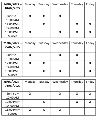
Over eight months, from the 15th of November 2021 until the 30th of June 2022, a minimum of two fieldwork sessions were carried out per day (five days per week). These two sessions were scheduled from a collection of three sessions (morning, midday, and afternoon), ensuring that sufficient data was collected across a range of temperatures (Table A1). Each fieldwork session lasted between two and three hours, with the aim of spending a total of five hours in the field per day.

During fieldwork sessions, giraffes were located via fresh tracks and faeces. Upon locating an individual or herd of giraffes, a fifteen-minute habituation session began, minimising the effect of observer presence on giraffe behaviour. During this habituation period, each individual was identified using the MRC giraffe ID kit.

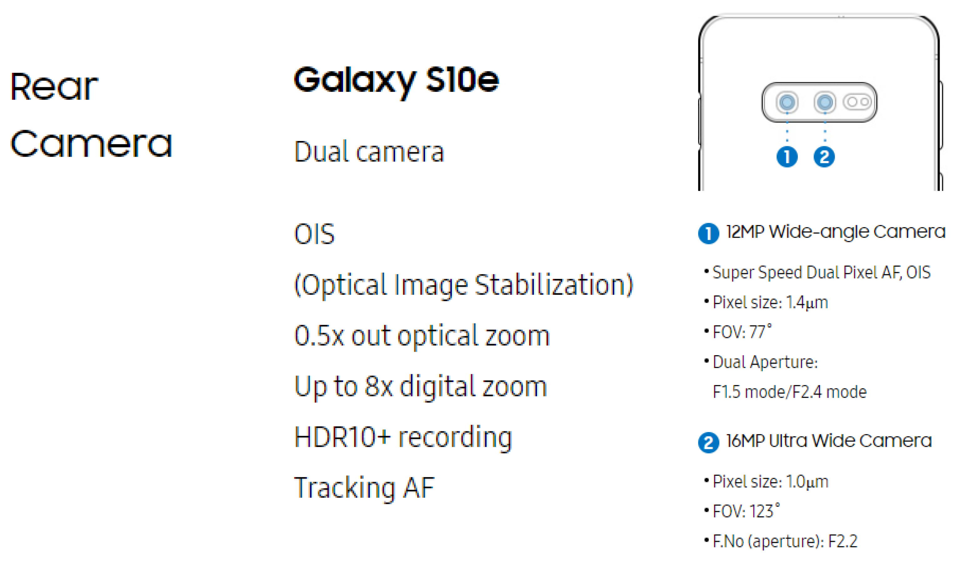
A photograph of each focal giraffe was also captured directly during the habituation process with a Samsung Galaxy S10e wide-angle camera (12MP; Figure A2), or indirectly, by directing the camera through a pair of binoculars, improving image quality for coat colour analysis. These photographs were also useful after the completion of a field session if identification of an individual was not possible. Each photograph aimed to capture an individual during full sun exposure, at side-profile, to prevent the darkening of spots via shade usage, or compression of spots during movements such as bending of the neck or body; in agreement with the work of Brand [27].

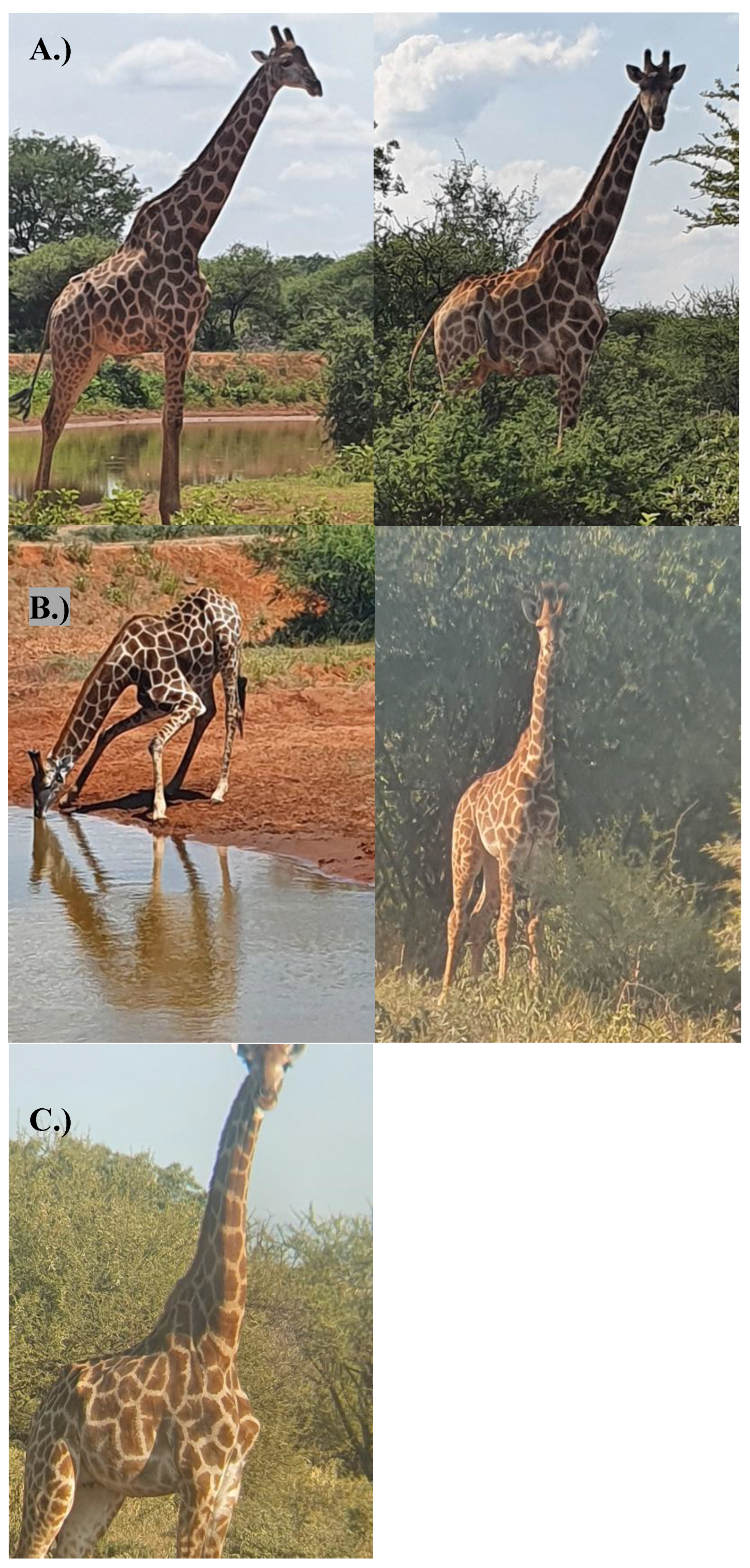
After the habituation period was completed, a ‘focal session’ began, whereby an individual giraffe was observed for fifteen minutes, whilst maintaining a safe distance. However, if an individual fled, a minimum of eight minutes was accepted, with time corrected for fifteen minutes after the field session. Data collected during a focal session included the following: time, date, name, sex and age of the focal individual, general behaviour, duration of time spent on each recorded behaviour, position of the individual with regard to the sun (towards, partially away, directly away), and sun exposure (full, partial, no exposure). Weather conditions were also recorded during focal sessions. Data was collected with a mobile application, AppSheet (version 1.000018; Figure A3). Several data categories, such as the position of the focal giraffe, required the judgement of the researcher within the field (Figure A4).

Daily minimum and maximum ambient temperatures were recorded using a thermometer (Figure A5) placed in shade. The maximum daily air temperature was used to test for significance in hypotheses surrounding temperature against position, temperature against coat colour, and temperature against shade usage.

2.4. Data Analysis

RStudio (version 4.0.3) was used for all statistical analysis. For the primary hypothesis of temperature against position, the relative time in each position was used, to assess which of the three positions were preferred as temperature increased. For further hypotheses, only the Relative Time Facing the Sun (RTFS) was used. This measure consisted of the proportion of each corrected 15-minute focal session that was spent facing the sun.

To ensure that the correct statistical tests were employed, Shapiro-Wilk tests were undertaken, observing the normality of each variable, with a critical value of 0.05 (α=0.05). The independence of samples was also tested by assessment, and if necessary, the equality of variance (α=0.05) was assessed using a Levene’s test.

The data underwent parametric or non-parametric tests, based on the results of preliminary analyses. A Spearman correlation was applied to observe trends in temperature against time spent in each position, temperature against coat colour, and temperature against shade usage. A Kruskal-Wallis test was used to assess significance for age (juvenile, sub-adult, and adult) against RTFS (α=0.05). A Wilcoxon-Mann-Whitney test was employed to assess significance in sex against RTFS (α=0.05).

For the analysis of age against RTFS and coat colour against RTFS, Dunn post-hoc tests were undertaken with Bonferroni correction, to assess for significant differences between each individual group. The time spent in each position and time spent in each exposure were also subject to linear regression.

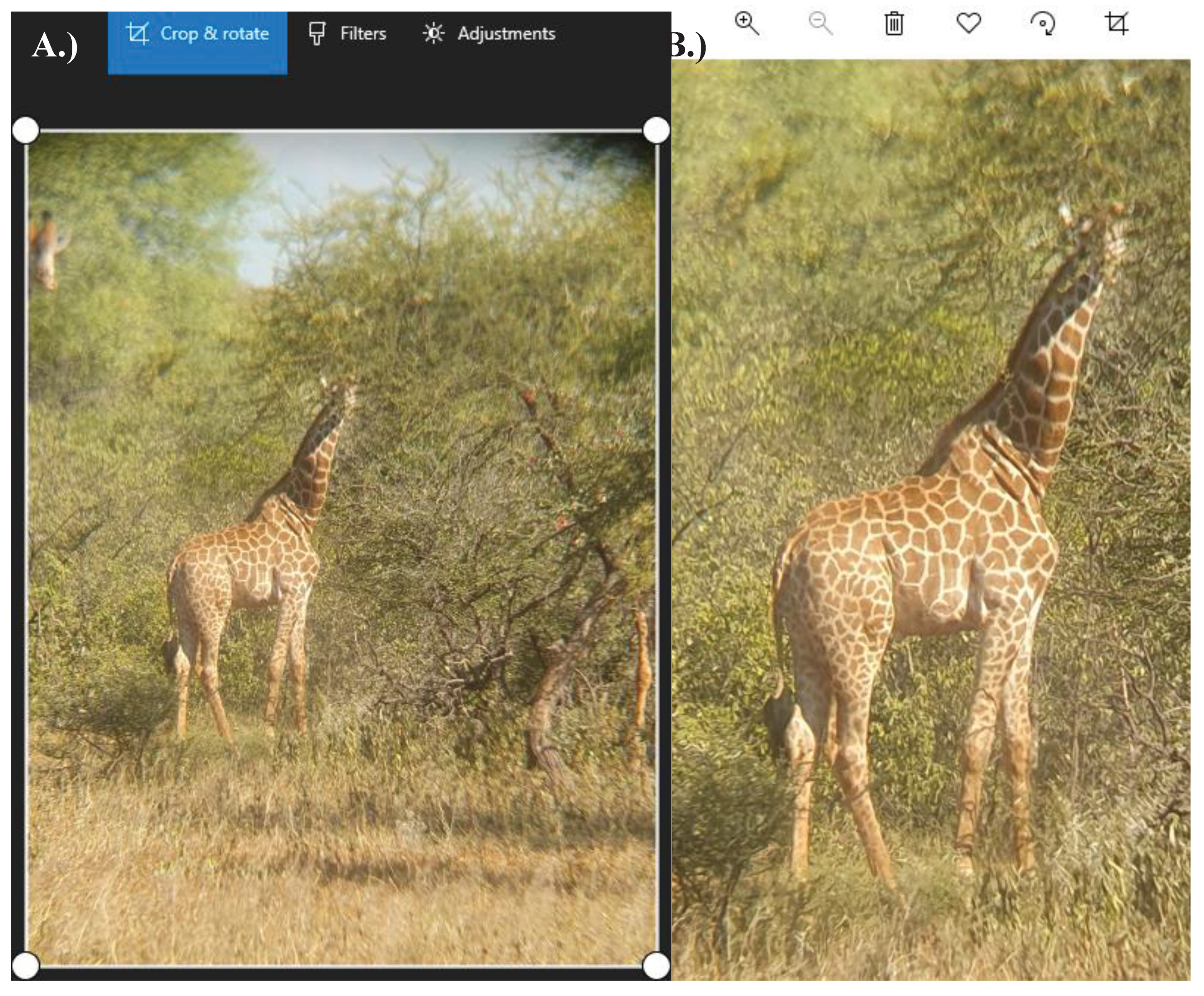
To determine giraffe coat colour, a series of steps were used. Firstly, photos taken in the field were edited, cropping out unnecessary background details (Figure A6), ensuring the key focus of each image was the focal giraffe. Poor quality images were not included in analysis (Figure A7).

Subsequently, an image file was uploaded to the ‘HTML Colors from Image’ webpage (‘https://html-color-codes.info/colors-from-image/’). This page was used to select a single point per image, from a dark patch on the middle of the giraffe’s neck or flank; this point was returned as a hexadecimal code, which represented coat colour as a string of characters (Figure A8). The hexadecimal codes were given in a #RRGGBB format, where each respective pair of characters denotes the proportion of red, green, and blue that make up any given colour.

Once two hexadecimal codes had been obtained for an individual, each code was entered into the ‘HTML Color Mixer’ webpage (https://www.w3schools.com/colors/colors_mixer.asp). This page created a colour gradient between two input codes, from which the ‘average coat colour’ code was obtained (Figure A9). This average code was recorded on a spreadsheet, alongside the two input codes.

Next, the average hexadecimal code was entered into the webpage ‘ColorHexa’ (https://www.colorhexa.com/). This site determined the ‘percentage lightness’ of the average hexadecimal code (Figure A10). This was also recorded on the spreadsheet.

For each image after the second, the same process was employed, with the exception that whilst creating a colour gradient on the HTML Color Mixer page, the new hexadecimal code (e.g., obtained from the third image of an individual) was mixed with the previous average coat colour code (e.g., the average from the first and second images of an individual). After each new image had been processed, both the old average coat colour and percentage lightness values were replaced by new values. A minimum of three and maximum of 15 images from each of the 55 sighted individuals were used in determination.

By the end data collection, an average of nine hexadecimal codes had been obtained for all observed individuals, providing a final average hexadecimal code and percentage lightness representing a coat colour for each giraffe.

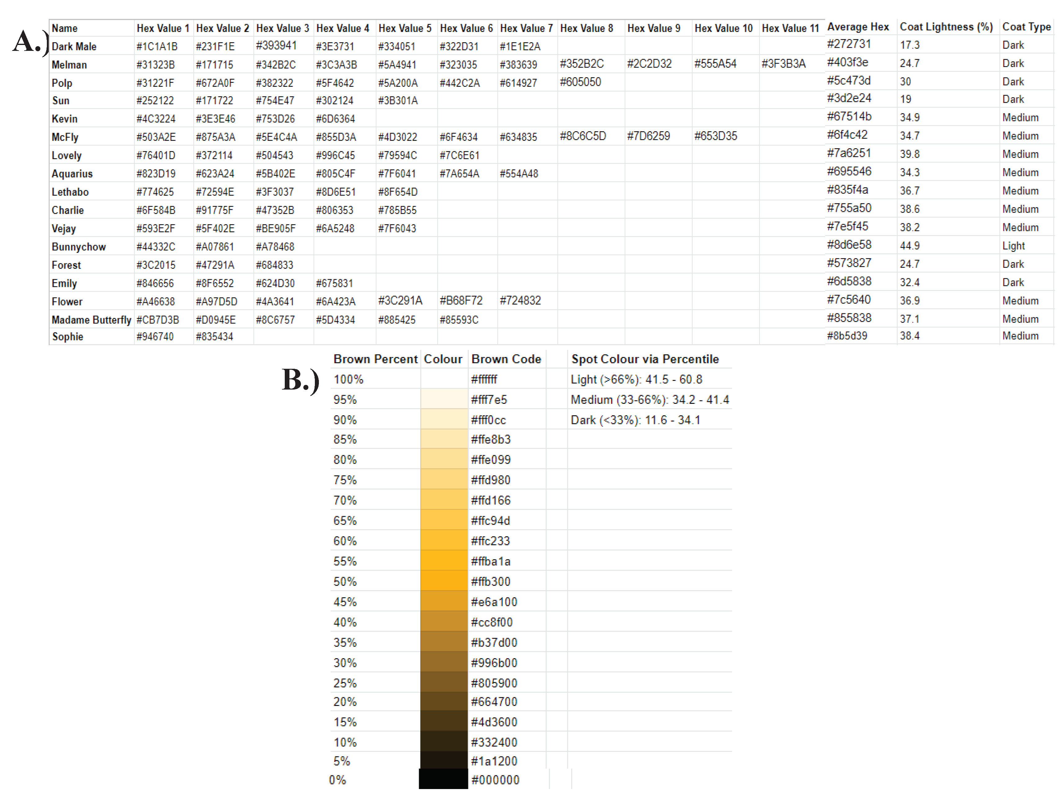
Finally, the final percentage lightness from each giraffe was used to create a percentage lightness scale. This scale was used to separate each giraffe into one of three coat colour groups, ‘dark’, ‘medium’, and ‘light’ (Figure A11), which were used in statistical analysis.

3. Results

3.1. Relationship between Temperature and Time Spent Facing the Sun

The data showed that as temperature increases, giraffes spend more time facing towards or away from the sun. To test the correlation between temperature and each of the three positions, normality was assessed using a Shapiro-Wilk test. The maximum temperature for combined positions was non-normally distributed (W=0.93, p-value <0.01). Similarly, the relative time spent in combined positions was non-normally distributed (W=0.97 p-value <0.01). This required the use of a non-parametric correlation test.

A Spearman correlation was used to test for significance between temperature and time spent in each position. The H0 (null hypothesis) was that the Spearman’s rank correlation coefficient, denoted as rho (ρ), was equal to 0. The ρ-value represents the correlation between the two tested variables. If the p-value was returned as ≤0.05, the H0 was rejected and H1 (alternative hypothesis) was accepted, indicating a significant correlation.

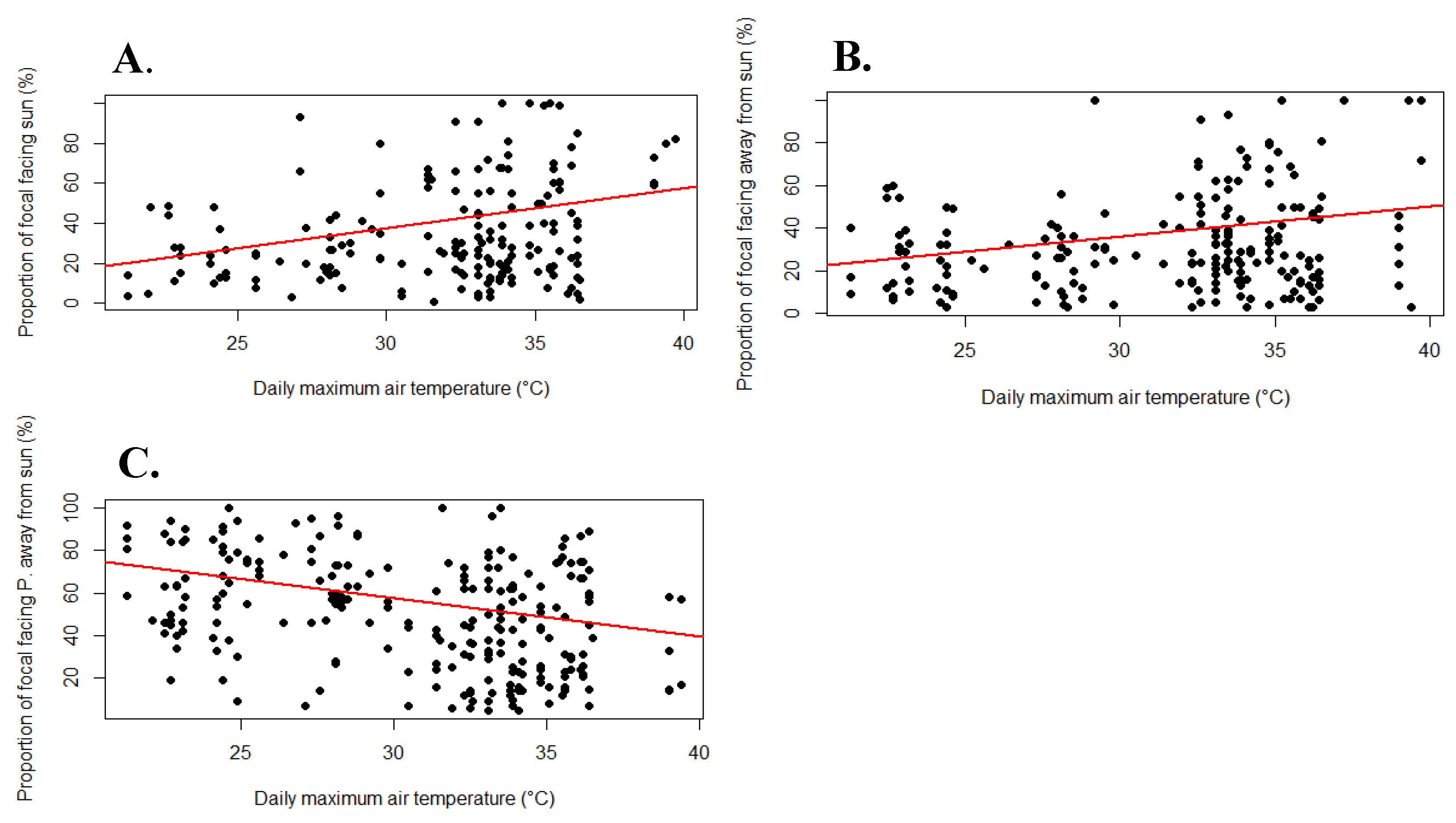
The values obtained from the correlation between maximum daily air temperature and the relative time spent in each position (Table 1) suggest that as temperature increases, giraffes spend more time facing towards (ρ=0.31, p-value <0.01) or directly away from the sun (ρ=0.19, p-value <0.01), and less time facing partially away from the sun (ρ=-0.36, p-value <0.01). Positive ρ-values signified a positive correlation, and negative ρ-values a negative correlation. Figure 2 displays the correlations plotted as linear regressions.

Time spent facing the sun had the strongest positive correlation (highest ρ-value), matching the hypothesis that giraffes prioritise facing the sun as temperature increases. This position was the only position regarded in subsequent tests.

3.2. Relationship between Age and Time Spent Facing the Sun

Statistical testing showed that adults and sub-adults spend significantly more time facing the sun than juveniles. The normality, independence, and equality of variance of samples, which included 376 adult, 74 juvenile, and 37 sub-adult observations were tested. Each group was found to be non-normally distributed (Shapiro-Wilk p-value ≤0.05). The groups were independent by assessment. Variance between age categories was unequal (Levene’s test p-value ≤0.05). Therefore, a Kruskal-Wallis test was undertaken with H0 ‘there is no difference between time spent facing the sun for different age groups’. For the Relative Time Facing the Sun (RTFS) H0 was rejected, a significant difference between age groups was detected (p-value ≤0.05; Table 2).

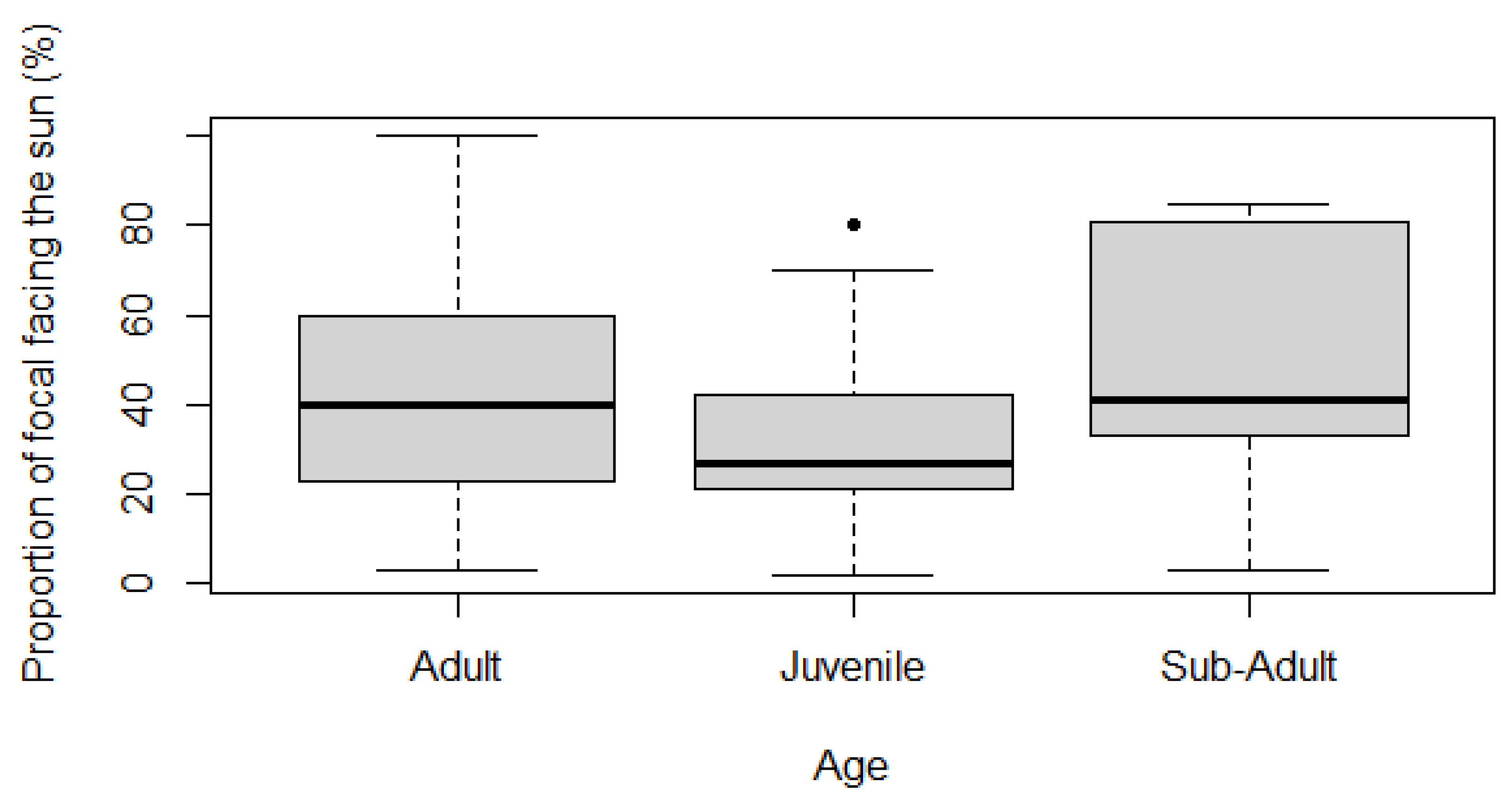
A Dunn test was then carried out to determine which groups were significantly different. The test found that sub-adults spent more time facing the sun than juveniles (p-value ≤0.05, negative Z-value), and adults spend more time facing the sun than juveniles (p-value≤0.05, positive Z-value) (Table 3), Therefore, it can be concluded that adult and sub-adult giraffes spend significantly more time facing the sun than juveniles (Figure 3).

3.3. Relationship between Sex and Time Spent Facing the Sun

Statistical tests suggest that males spend significantly more time facing the sun than females. The normality, independence, and equality of variances were examined to determine which test was required. The RTFS was non-normally distributed for both sexes (Shapiro-Wilk p-value ≤0.05). The data was independent by assessment. The variance between the sexes for RTFS was not equal (Levene’s test p-value ≤0.05) (Table 4).

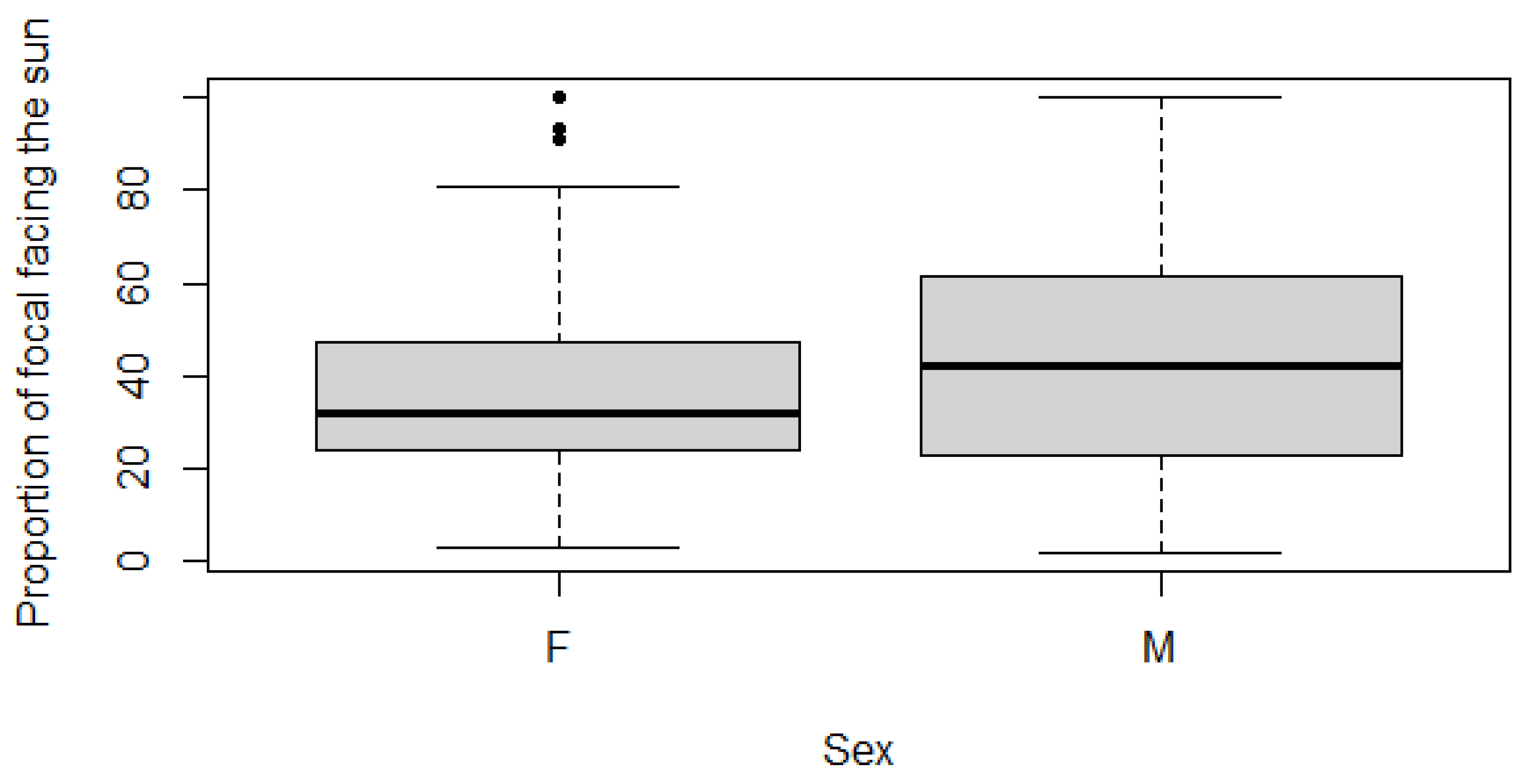
From the assessment of data, a Wilcoxon-Mann-Whitney test was required. H0 was ‘there is no significant difference in time spent facing the sun between sexes’. For RTFS, H0 was rejected, there is significance difference within sex and time spent facing the sun (p-value ≤0.05), (Table 4). Visual representation of the data along with prior statistical tests revealed that males spend significantly more time facing the sun than females (Figure 4).

3.4. Relationship between Coat Colour and Time Spent Facing the Sun

The results suggested that giraffes with darker coats spend significantly more time facing the sun. Each of the three colour groups (light, medium, dark), along with previously tested variable, were non-normally distributed (Shapiro-Wilk p-value <0.05). The three colour groups were independent by assessment, and variance between groups was found to be unequal (Levene’s test p-value <0.05) (Table 5). Therefore, a non-parametric Kruskal-Wallis test was used to test for significant differences between the groups, with H0 ‘there is no significant difference in time spent facing the sun for different coat colours’.

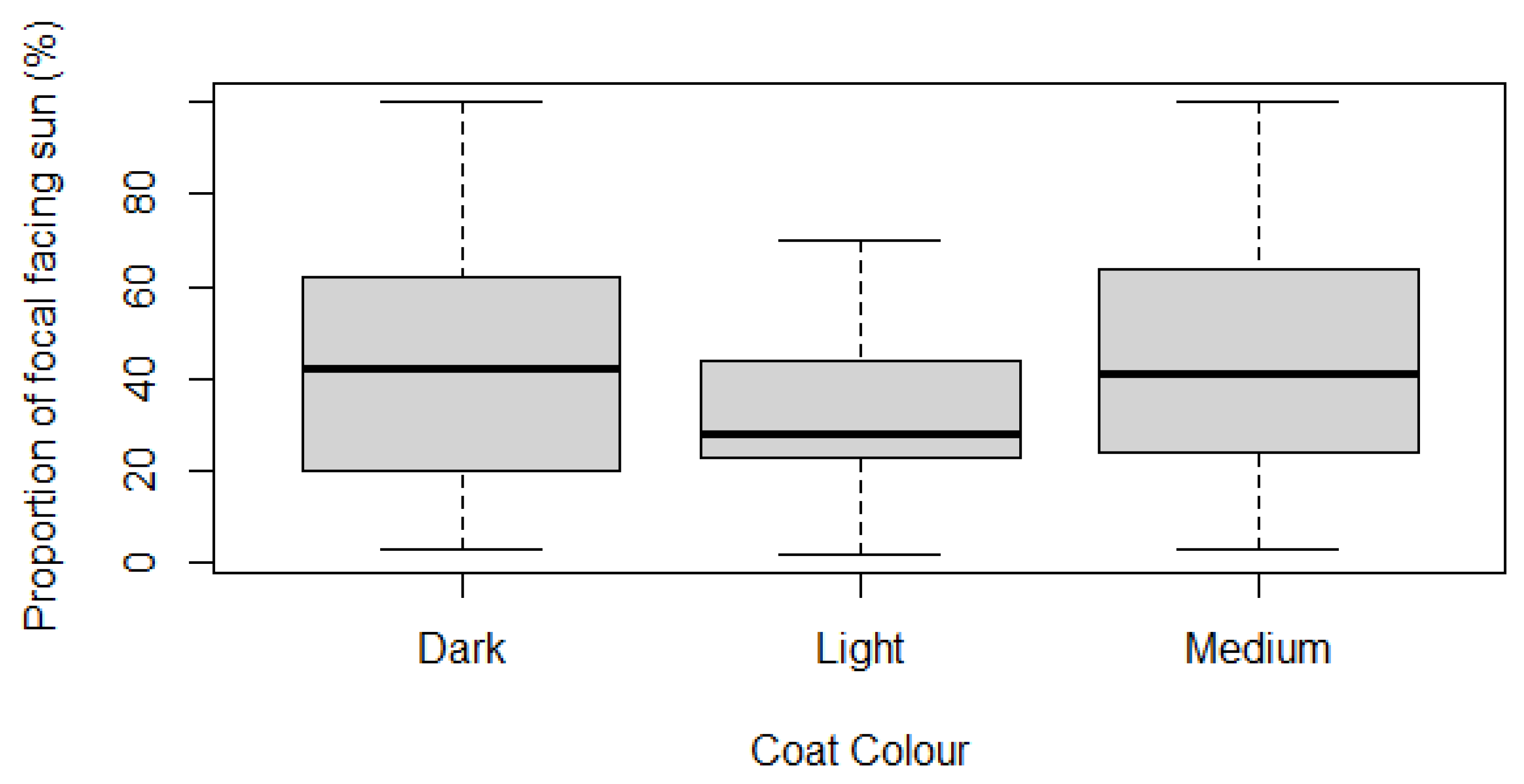
H0 was rejected, and significant difference was identified between RTFS and different coat colours (p-value <0.05). A Dunn test was carried out to determine where significance occurred (Table 6). It was observed that dark-coated individuals spend significantly more time facing the sun than light-coated individuals (p-value≤0.05, positive Z-value) and light-coated individuals spend significantly less time facing the sun than medium-coated individuals (p-value≤0.05, negative Z-value). Therefore, it can be said that giraffes with darker coats spend more time facing the sun. Boxplots were used to visualise the difference between each group (Figure 5).

The average Percentage Coat Lightness was predicted to differ significantly between males and females; however, this was disproven (Males = 37.7%, Females = 38.8%).

3.5. Relationship between Temperature and Shade Usage

The data suggested that as the temperature increases, giraffes used shade significantly less. The Relative Exposures per Focal (REF), which consisted of the relative time spent in all combined exposures was tested with a Shapiro-Wilk test and was found to be non-normally distributed (W=0.93, p-value <0.01). Previously tested variables, RTFS and Maximum temperature were also non-normally distributed, therefore, a Spearman correlation was required. The H0 hypothesis was ‘ρ=0’, if the p-value was returned as ≤0.05, the H0 was rejected, and a significant correlation was present.

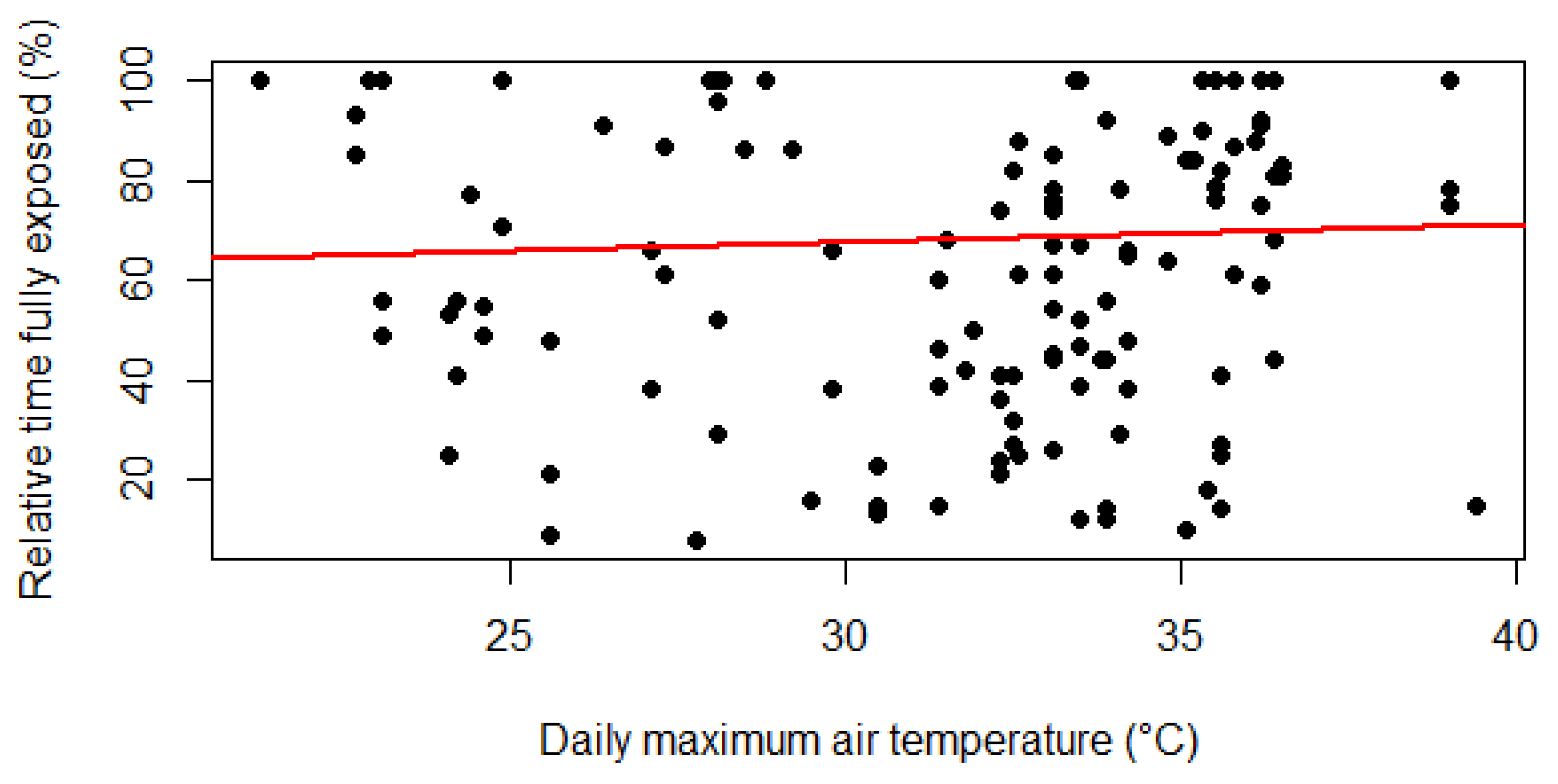
From the results of the correlation (Table 7), there was a significant trend between maximum temperature and full exposure (ρ=0.16, p-value <0.01). These results suggested that as temperature increases, giraffes enact more behaviours in direct sunlight, disregarding the shade of trees and other giraffes. This finding was visualised as a regression plot, displaying the positive trend between full exposure and maximum temperature (Figure 6).

3.6. Relationship between Seasons and Time Spent Facing the Sun

Statistical tests determined that giraffes spend significantly more time facing the sun during the wet season. The normality, independence, and equality of variables was first tested to determine which test would be most effective. The RTFS was abnormally distributed for each season (Shapiro-Wilk p-value ≤0.05). The data was independent by assessment. The variance between seasons for RTFS was unequal (Levene’s test p-value ≤0.05) (Table 8).

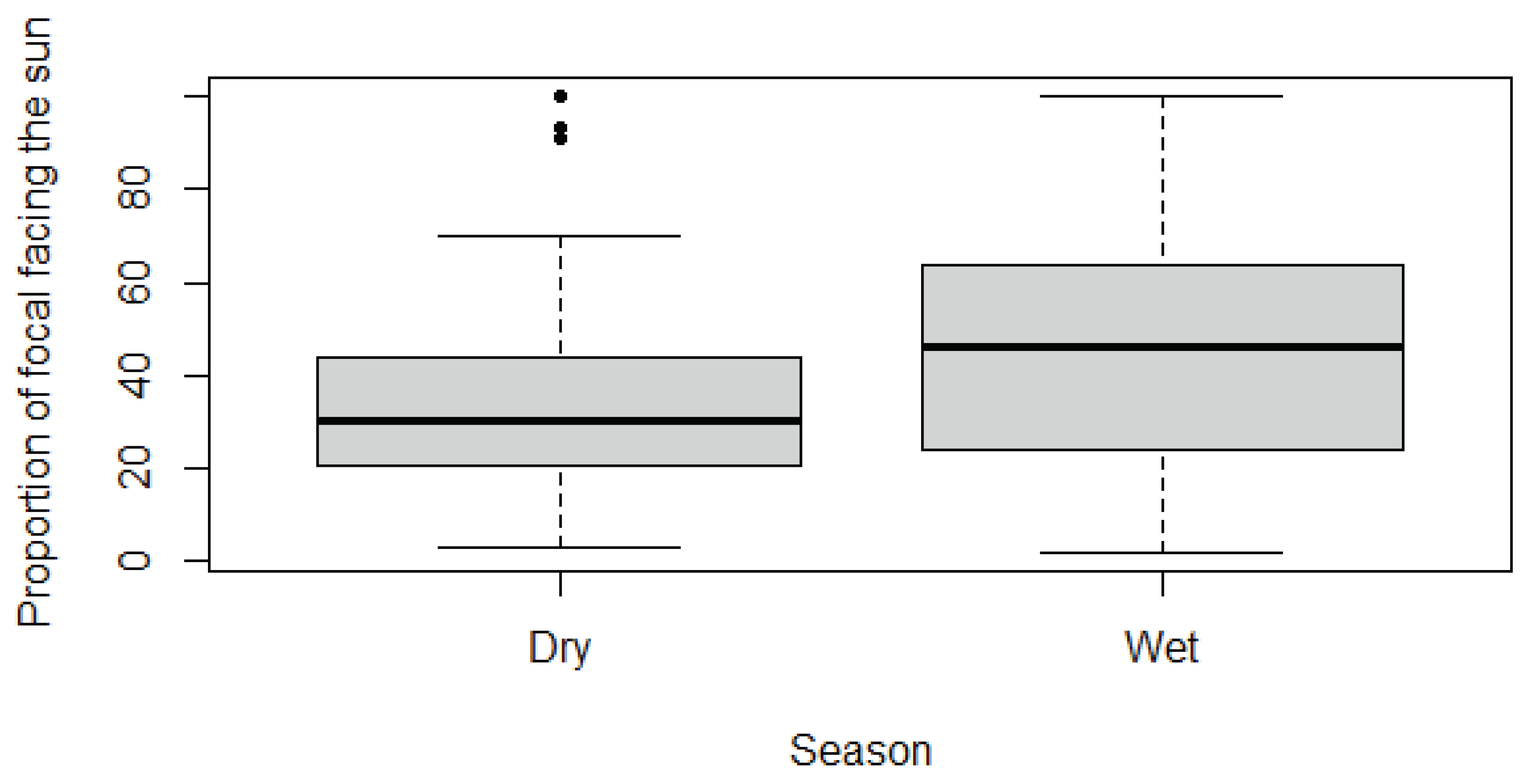
Using the assessment of variables, a Wilcoxon-Mann-Whitney test was required. The H0 hypothesis was ‘there is no significant difference for time spent facing the sun between seasons’. For RTFS, the H0 was rejected, there was a significant difference between time spent facing the sun and season (p-value ≤0.05; Table 8). This data was visualised with boxplots that suggested more time is spent facing the sun in the Wet season (Figure 7).

4. Discussion

The results from the study on behavioural thermoregulation in giraffes demonstrated the main hypothesis that as temperature increases, time spent facing longitudinally (anterior or posterior [19,28]) to the sun increases. This was displayed by the significant increase in time spent facing toward or away from the sun, and the significant decrease in time sent facing partially away from the sun (Figure 2).

During the study of Kuntsch and Nel [28], the majority of observations were recorded at summer highs of 35°C, and winter highs of 16°C. Conversely, the summer period comprising the main dataset of this study displayed an average temperature of approximately 30°C (Figure 1). This meant that less data was available for higher temperatures, especially those closer to the giraffe internal body temperature of 38.5°C [29]. This may have weakened any observed trends regarding time spent facing the sun as temperature increases, however, the same trends were observed, showing that the change in behaviour occurs over a smaller temperature range than expected.

Kuntsch and Nel [28] also found that there were significant differences between the sex or age of a giraffe, and the time spent facing the sun longitudinally. Juveniles were found to spend significantly less time facing the sun compared to adult individuals. This finding acts in agreement with the current study, which found that adults and sub-adults spend significantly more time facing the sun than juveniles (Table 3). There was some overlap of the boxplot results, and noticeable standard deviations (Figure 3). The overlap of results suggests that differences between the groups may only be small, and the large standard deviation was expected, due to the collection of data across a large temperature range; providing a proportion of time facing the sun that is not clustered around a mean value.

Despite concurrence, the conclusion reached in the current study may be subject to scrutiny, due to sample sizes. Adult individuals made up 376 of the total observations, whereas Juveniles made up 74, and Sub-Adults only 37. Without secondary literature, the unequal and small number of samples may have led to inaccurate trends, most notably within the sub-adult category. This issue arose due to the small number of sub-adult giraffes on the reserve; however, this could be solved by studying a community with more sub-adults or correcting for the smallest sample number. Similarly, multiple individuals within the MRR had approximated ages, with greater accuracy for juveniles born during the time of the study. This approximation may have led to the incorrect age categorisation, allowing for reduced sample sizes of smaller age groups, such as sub-adults. In future works focusing on the age of individuals, precise ages may be advisable to maintain accuracy in conclusions.

Regarding the sex of giraffes, Kuntsch and Nel [28] ventured that males spend significantly more time facing the sun. The current results also found that males spent significantly more time facing the sun (Table 4; Figure 4). There is a large overlap within the boxplots which suggests that the effect is minimal.

The work of Kuntsch and Nel [28] excluded non-adult individuals from sex-based conclusions, whereas the current work included every age category, even assigning sexes to juveniles that could not be sexed reliably. This was done by assessing the proportion of males and females born to each family tree, and image analysis of individuals. This method may have led to false attributions of sex, which in turn gave the weak significant difference observed. To combat any errors this may cause in future works, the use of only known-sex individuals may be advisable.

One reason hypothesised as to why males face the sun more often was that of coat colour. It was assumed that on average, male giraffes would have darker coats than females. This would increase the time spent facing the sun to combat the increased absorption of solar radiation associated with darker colours [30]. This conclusion considered secondary literature, however these commonly focused exclusively on the male giraffe. Similarly, disagreements on how coat colour changes with time, primarily in males, occurred frequently [31,32]. To assess how the coat colour differs between males and females on the MRR, the average coat colour of each sex group was determined. It was found that the average coat colour, represented by Percentage Coat Lightness, was similar between sexes (Males = 37.7%, Females = 38.8%). The lack of difference between the average coat colours may suggest that coat colour has a negligible effect on the time spent facing the sun regarding the sex of an individual.

Independently of sex, coat colour was found to have a significant effect on time spent facing the sun, with the data proving that darker individuals spend more time facing the sun (Table 6; Figure 5). The boxplots show partial overlap, which may be due to the inclusion of individuals with coat colours that lie on the boundary between two coat colour groups. The large standard deviations observed in the medium and dark colour groups may be due to the larger number of individuals classified in these groups, providing a more random spread of data compared to the smaller light category.

Darker individuals likely face the sun more as compensation for the increased rate of heat absorption that comes alongside the benefits of a darker coat, such as the perceived dominance of males. Further work is necessary to understand the mechanisms of coat colour in giraffes, independently and regarding the sex of an individual. This work is especially important in females, which are often excluded from research on coat colour.

When observing the shade usage of giraffes, it was found that individuals spend significantly more time in full sunlight as temperature increases (Table 7; Figure 6). This may suggest that thermoregulatory behaviours such as facing the sun are sufficient to maintain a stable internal temperature as external temperatures increase. This data opposes previous works by Brand [27] and Kuntsch and Nel [28] which suggested that as temperature increases, time spent facing the sun and time spent seeking shade increases. This may also have links presence of cloud cover in the 2022 study.

Kuntsch and Nel [28] observed that females and juvenile individuals spent more time seeking shade, whereas the current study looked at shade usage in giraffes as a whole and did not split the data into sex or age with regard to shade-seeking. Kuntsch and Nel [28] also suggested that as the availability of direct water and water from food sources increases, certain behaviours such as facing the sun and seeking shade would decrease, as non-behavioural methods to mediate temperature have been introduced. This may have led to the differences in results, as the reserve provides a constant source of water in the form of man-made waterholes, and rainfall has been spread over a longer period of the year, into the dry season. This increased availability of water may have drawn giraffes in the study group to spend extended time without seeking shade, especially in open areas, where shade was not present. In these areas water was obtained directly and indirectly, thus the necessity for shade usage was decreased, opposing the increased requirement for facing toward or away from the sun.

The difference between shade-seeking and identity is also noted by Brand [27]. Pale males were found to have sought more shade than dark males and females during hot summer months, and dark males and females were found to seek more shade in colder winter months. However, Brand [27] also identified that giraffes as a whole sought more shade during cloudy days, “possibly because of the reduced directionality of incident sunlight”. This restricted the analysis to days where the cloud cover was a quarter or less. In the current study, analysis of shade usage completely excluded cloudy days, as an attempt to keep consistent with analysis of position and time spent facing the sun, which also included only sunny days. The differences between the division of giraffe identity and inclusion of cloud cover in separate works may have caused the differences observed between results. These differences may be resolved by dividing the current data regarding shade-seeking collected on the reserve into age, sex, and coat colour. Further research with a greater focus on weather conditions such as cloud-cover may also be undertaken.

Seasonal differences were observed to assess any annual trends in giraffe thermoregulatory behaviours. The results found that giraffes spent a significantly higher proportion of time facing the sun in summer months, compared to winter months (Table 8; Figure 7). This follows the established hypotheses and can be explained by the increased temperatures observed during the summer season (Figure 1); This links to the first hypothesis, that giraffes face the sun more as temperature increases.

The observed seasonal trend may be useful in predicting how the proportion of time spent facing the sun will change in future, when temperatures have been altered via the action of global warming. Similarly, this trend may allow for effective comparisons between previous works, and future studies.

As the current study was carried out over 8 months, the time available for data collection during winter months was reduced. This increased difference in sample numbers between summer and winter may reduce confidence in seasonal trends. This calls for further research to cover the entire course of a year, or more, to obtain equal samples across full seasons.

This winter data was also affected by the increased cloud cover during the winter months of 2022. Many days during winter were recorded as ‘cloudy days’, where determining the position of an individual relative to the sun was difficult, if not impossible. The increased cloud cover may also make the comparison to alternative research such as that of Brand [27], who factored in cloud cover to their work, less reliable.

One issue that affected data collection was the use of AppSheet. This application allowed data to be automatically uploaded to a spreadsheet, making collection more efficient and providing parity to methods employed in previous works on the MRR. However, due to bugs, ongoing maintenance of the data collection application was required, and individual behaviours often took time to record, making short-lived behaviours difficult to collect. This may have affected results by decreasing the number of observed behaviours and increasing the length of others. This may be solved by using field-notes or identifying better software for data collection.

Another complication was the subjectivity of variables. Steps such as mimicking the direction of the giraffe to accurately identify the position relative to the sun were taken, however, the study observed several variables differently to previous research undertaken on the reserve [33,34,35], making comparison between works difficult. Similarly, the time taken to determine the position and weather made the collection of short-lived behaviours challenging. This led to the decision to remove the wind category, which was assumed to have little effect on thermoregulatory behaviour, due to the lack of wind observed across the study period. These problems may be minimised by considering the opinions of multiple field researchers when recording subjective data categories.

The number of individuals on the reserve was also thought to have had an effect on behaviour. The carrying capacity of giraffes on the reserve, based on size consideration, was found to be 6 individuals [36]. Throughout the study, the number of giraffes on the reserve increased from 50 to 57 individuals, 55 of which were studied. This may have had an effect on the behaviour of the study group, as giraffes were often found in highly social groups of up to 15 individuals. These large groups could have had an impact on the types of behaviours observed. Prioritisation of social behaviours, for example necking and mating, and a reduction in vigilance behaviours in these large groups [37] may have been encouraged by the close proximity of so many dominant individuals.

The time spent facing the sun may have been affected by the vigilance behaviour of giraffes. A habituation session was put in place to reduce the overall vigilance of giraffes to the observer, and a reasonable distance was maintained from individuals during focal sessions, however, there was no feasible means to completely prevent wariness towards the researcher. The initiation of vigilance behaviour to the researchers often meant that other thermoregulatory behaviours were cut short, and during vigilant periods, the individual often ‘froze’ in place or fled, leading to significant proportions of a focal session spent in a position that would otherwise not have occurred, or cutting the focal session short.

5. Conclusions

The field collection and data analysis on behavioural thermoregulation in giraffes displayed ample concordance with previous research, with a handful of differences that may be explained by the context of the research, such as recent weather patterns and the location of the work.

Giraffes displayed interest in positioning themselves laterally to the sun on higher temperature days, with a predicted preference for facing anteriorly to the sun, casting shade over the main bulk of the body during full exposure. This behaviour was divided according to hypotheses regarding the identity of giraffes, with males and darker individuals facing the sun for longer periods than females and lighter individuals. The only identity that showed unexpected results was sub-adults, which were found to spend more time facing the sun, which were explained by the sample number of the study. The thermoregulatory behaviours studied were also found to follow a seasonal course, with more time spent facing the sun during the winter, where temperatures were lower.

Finally, the shade usage of giraffes was found to be negligible, with a slight preference for full exposure on hot days. This suggested that the behaviours studied were crucial in maintaining a stable internal body temperature, above other options.

These results may be instrumental in the commencement of further works on giraffes as a species, determining further taxonomic differences between individuals that may aid in settling the question on the existing number of species and sub-species, and the action through which these sub-species are formed. Similarly, future works may find it important to place greater focus on identities less represented in general research, such as females and sub-adults.

This understanding may also help in the conservation of groups of giraffes that are vulnerable or endangered. The creation of environments where the need for thermoregulatory behaviours is reduced may alleviate the stress on individuals, leading to more efficient breeding programmes, and reduced mortality rates. This may provide a necessary boost to local population numbers, which in turn could allow for transfer of individuals into separate locations, where genetic disparity could be bolstered. This would lend further resilience to struggling populations, where alteration of the environment is not possible, or would damage the biodiversity organisms other than the giraffe.

Funding

This research received no external funding.

Data Availability Statement

Data can be made available on request.

Acknowledgments

To begin my acknowledgements, I would first like to thank my supervisor Grietjie Stander for her unquestioning assistance in my research and the creation of the materials that will be used in my academic assessment. Throughout my extended time at the Mogalakwena Research Centre, there were times where my work was attempted as independently as possible, however, in so many cases where any questions formed, or the focus and motivation within my research became uncertain, Grietjie provided all the help that could possibly be asked for, and even gave advice intuitively when it became outwardly apparent that I had an issue that I thought I should solve; seeing as it was of my own creation. Similarly, I would also like to thank other supervisors, Dr Tanja van de Ven, and Berenger Laurent, for providing further insights into the work I have carried out, making me feel like a true scientific peer, over a temporary intern. Secondly, I’d like to thank the Coetsee family for creating the River Reserve, and other protected areas that aim to contribute to the ongoing fight for conservation. These areas have been transformed into amazing environments for the study of wild animals, which very few get the chance to visit and complete research on. Each member of the family has been very caring to me and other students on the reserve, offering ample insights into the various different roles it takes to maintain a reserve in the harsh South African bush. On top of this, many personal anecdotes have been provided by each individual within the family, defining them not only as the creators and caretakers of the reserve, but passionate people with captivating stories and ideals inside and outside of their lives’ work. Next, I’d like to thank the students who surrounded me on a day-to-day basis, supporting me in both social and professional contexts. My special thanks go to Camille Chalas, for providing quality images of some of the new juveniles born within my time on the reserve, helping me to edit the Mogalakwena giraffe ID kit for future students. Similarly, I thank Bastien Macé, Elisa Vassas, Elodie Courtel, and Elsa Marçon, for all of the help they provided at the beginning of my work with giraffes, it would have been impossible without them. Special thanks are also in order for every other individual I met during my time within the Mogalakwena research centre, however, due to the length of my placement, I have met so many amazing people, with the most immense variation of journeys and destinations; so, I take this time to thank you all individually for providing something different to my life, shaping it in the most important ways. Additionally, I would like to express my gratitude to the University of Cardiff and my personal tutor, Isa-Rita Russo. Isa-Rita provided a great deal of help in finding a placement, suggesting the Mogalakwena Research Centre amongst other locations. I’d like to believe that she is the main reason I ended up at the research centre, where I have had the most amazing experience. My university also provided a lot of help with the financial and planning aspects of my placement year, helping to lessen any anxieties I had with the extensive preparations for a placement relatively far from home. Finally, I would like to thank my family and friends in England. I have had constant support from a multitude of people throughout my life, pushing me to carry on and fight to get to the point where I was able to undertake such an immense experience. The support has continued, even from so far away and I cannot stress the strength that I have drawn from all of these individuals who have made my regular life worth living.

Conflicts of Interest

The author declares no conflict of interest.

Appendix A

Figure A1. Maps displaying South Africa, Limpopo, and Mogalakwena. A.)(TUBS, 2011). A map depicting South Africa, separated into nine constituent provinces. Highlighted in red is the Limpopo province, where the study area resides. B.)(Htonl, 2016). A map depicting the Limpopo province, divided into five district municipalities, indicated by bold intersecting lines. Municipalities are further broken into twenty-two local municipalities, indicated by the fine intersecting lines. The local municipality highlighted in red is the Mogalakwena municipality, where the Mogalakwena River Reserve resides.

Table A1. Field Schedule Tables. To accommodate a minimum of two field sessions per day, as set out in protocol, a three-week schedule from the 14^th of February until the 4^th of March 2022 was drawn up. Over the course of three weeks, this rotation allowed for an equal number of sessions, marked by an X, across each period from sunrise to sunset. Consequently, the volume of data collected across days will remain relatively equal.

Figure A2. Image Capturing Device and specifications (Samsung Electronics [no date]). A photograph of each giraffe encountered in a session was required for two purposes. One purpose was for determination of the coat colour of each individual. The other purpose was for determining the identity of individuals if identification was not possible prior to, or during, a focal session. Due to a lack of specialised imaging equipment, the device used to capture these photographs was a Galaxy S10e, with two rear cameras. The Camera used was the 12MP wide-angle camera, with its respective statistics. This quality allowed for photographs to be taken for use in preliminary studies on coat colour.

Figure A3. Layout of AppSheet software. During this work, an application was required for data collection. A.) The free version of the app development platform ‘AppSheet’, found at: https://www.appsheet.com/, provided all the tools necessary to create a mobile application for fieldwork. B.) Each column in the prototype application ‘Behavioural Thermoregulation’ represented a data category observed during fieldwork. For each category, the type of data that could be entered into the mobile application was specified.

Figure A4. Identifying giraffe positions relative to the sun. A.) Whilst facing ‘Directly away from the sun’, the back was fully exposed to the sun, with the front fully cast in shade. The sides may also be partially cast in shade. B.) Whilst facing ‘Partially away from the sun’, the majority of one side of the body was exposed to the sun, with the other side primarily cast in shade. Any shadow cast onto the floor was also offset to one side, not directly to the front or back. C.) ‘Toward the sun’ was characterised by full sun exposure on the front of the body, with shade cast over the back via the elongated neck. The sides may have been cast in partial shade but were still often exposed to a degree of sunlight.

Figure A5. Thermometer and specifications (Takealot Online (Pty) Ltd. [no date]). To correctly measure the maximum daily air temperature, a precise thermometer was required. This thermometer measured the temperature to one decimal place, with an accuracy 1°C either side of the true temperature.

Figure A6. Pre-edit and Post-edit giraffe photographs. A.) In the unedited photograph, the subject giraffe took up little of the shot, leaving room for background details that were not used in coat colour determination. This photo was cropped to ensure that the focal giraffe took up the majority of the image. B.) In the edited photograph, the subject giraffe took up the whole image. This allowed for easier pixel selection during the conversion of visual colour to hexadecimal code.

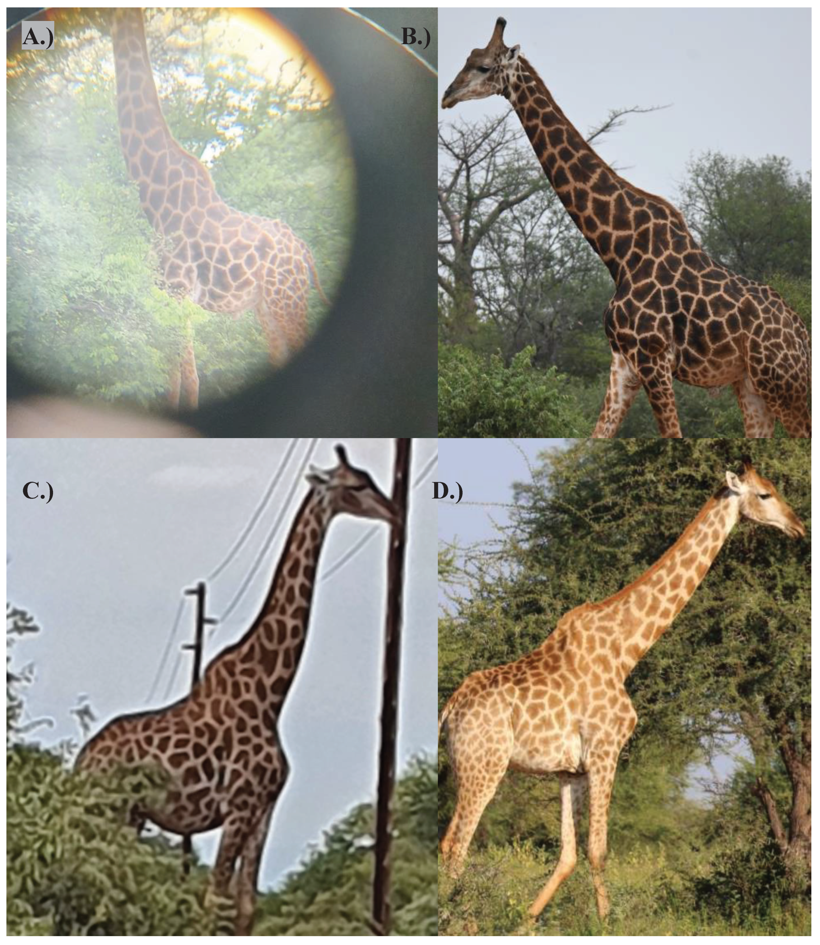
Figure A7. ‘Poor’ quality images versus ‘High’ quality giraffe photographs. A.) In the first image, the subject, ‘Polp’, was too far for a quality image to be taken with the imaging device. A pair of binoculars was used in addition to the imaging device in an attempt to capture a clearer image. The use of binoculars created a visible around the subject, which was removed via editing, and a visible white hue, which couldn’t be removed. This photo was discarded, as the hue effected the coat colour output in further steps. B.) In the second image, there was no hue present, which allowed for an accurate coat colour to be determined. C.) In this image, the subject, ‘Madame Butterfly’, was captured at a low light level, due to poor weather conditions. This caused an unfocused image to be captured, which needed to be discarded. D.) In the final image, the subject, ‘Madame Butterfly’, was captured at an adequate light level. This produced a high-quality image which was used when determining an average coat colour.

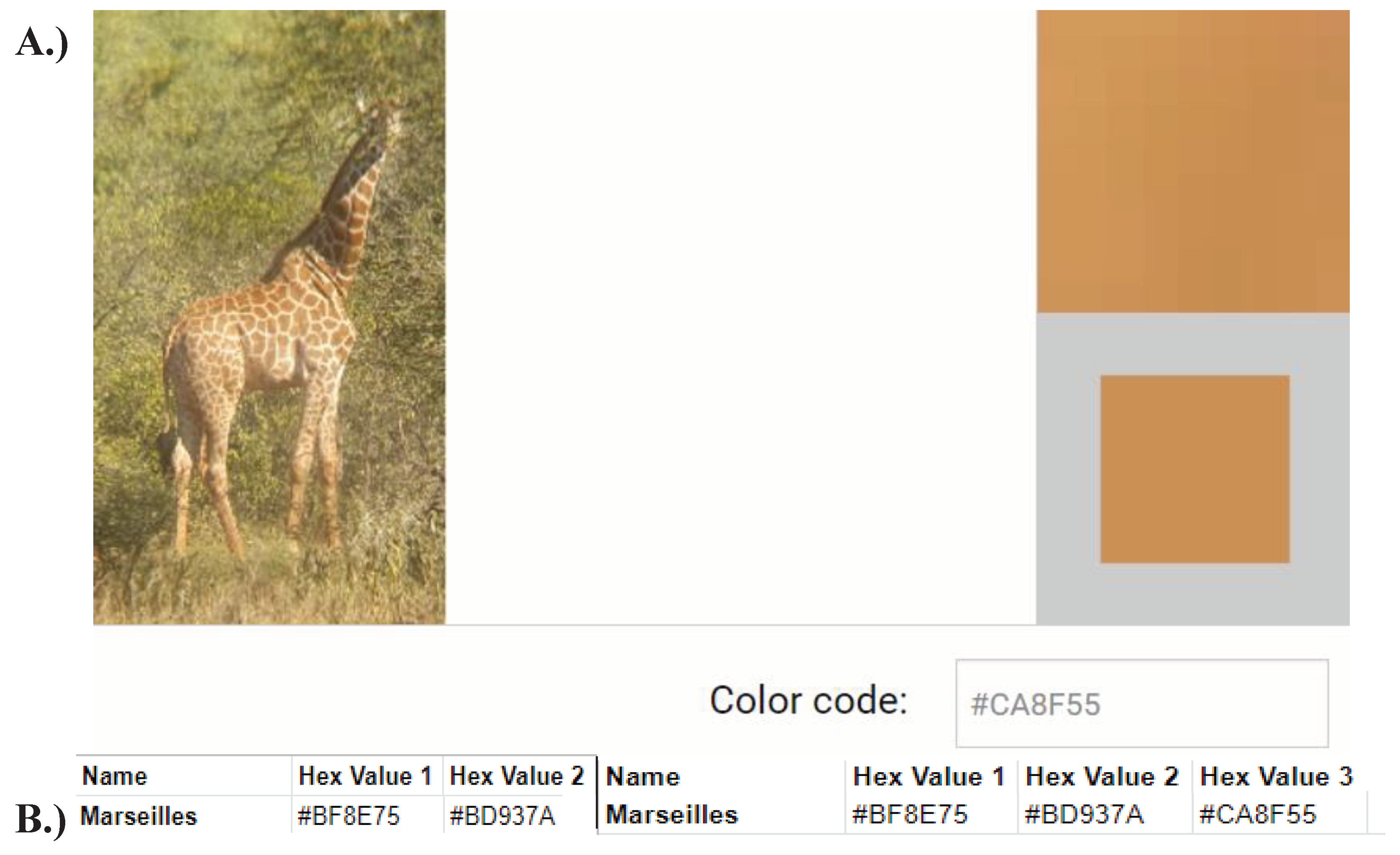
Figure A8. Obtaining a hexadecimal code from edited images. Hexadecimal codes come in #RRGGBB format, which represent the proportion of red, green, and blue, that make up any colour. Hexadecimal codes are more convenient to work with than binary, which are comprised of complex strings of ones and zeros. A.) Subsequent to image editing, the website found at https://html-color-codes.info/colors-from-image/ was used select a single point from an uploaded image. This provided a matrix of pixels displayed in the upper right-hand, which was used to select a single pixel, displayed in the lower right-hand corner. This pixel was provided with a corresponding hexadecimal code, for example ‘#CA8F55’. This code was used in further steps to determine coat colour B.) A spreadsheet was used to record all hexadecimal codes. For example, the code ‘#CA8F55’ was obtained from the third image of Marseilles and was used to determine the second new average coat colour of the individual.

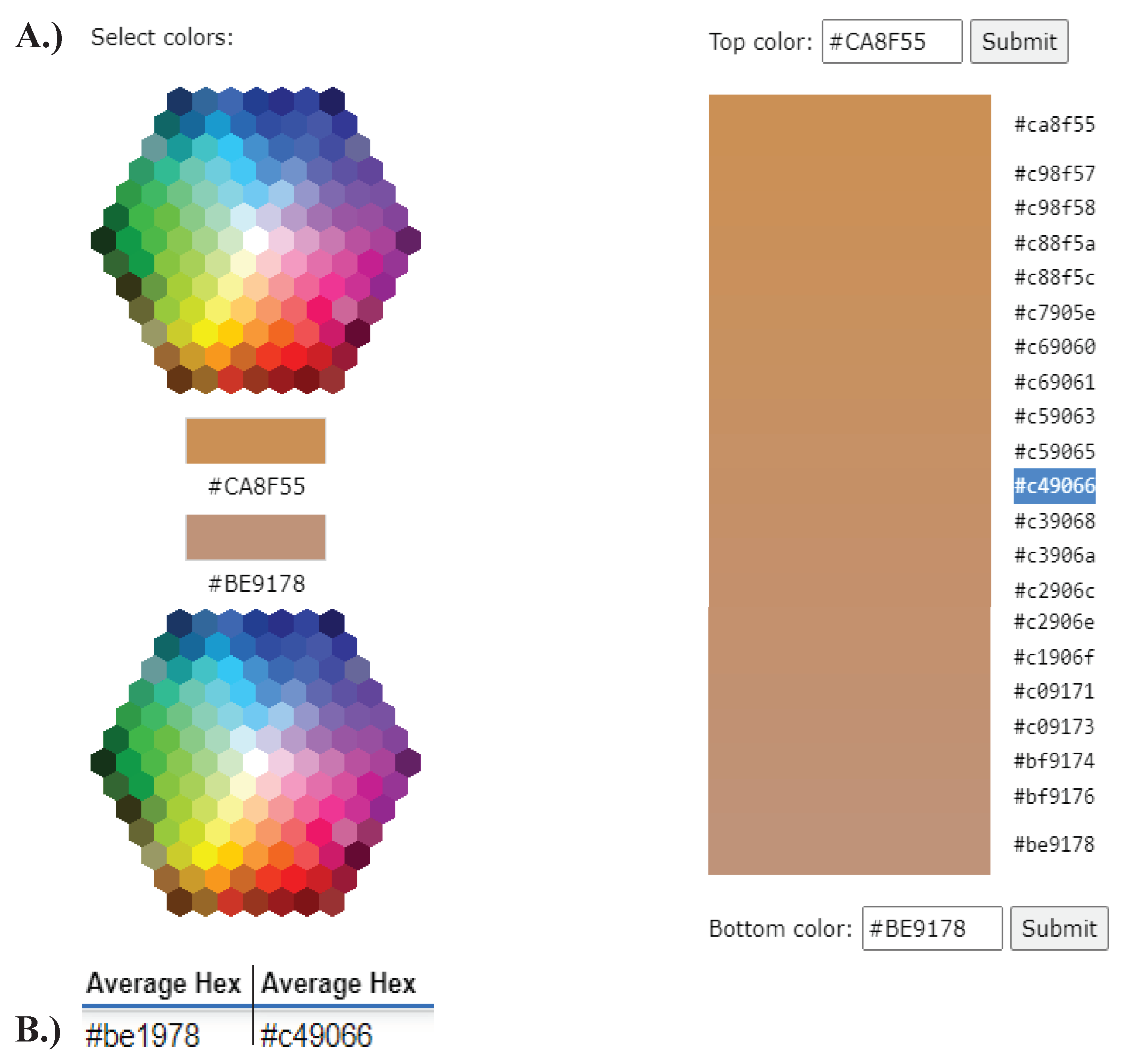
Figure A9. Creation of a new average hexadecimal code using gradients. A.) After determining the hexadecimal code from an edited image, a new average coat colour needed be calculated. This was done by entering the old average hex code, for example ‘#BE9178’, and the new average hex code, for example ‘#C49066’, into the website found at: https://www.w3schools.com/colors/colors_mixer.asp. The output was a colour gradient and corresponding hexadecimal codes, from which the central, or average, code was selected. The code in the provided example (‘#C49066’) was then used in further steps to determine coat colour. B.) Examples of the old average hex code on the left-hand, and new average hex code on the right-hand.

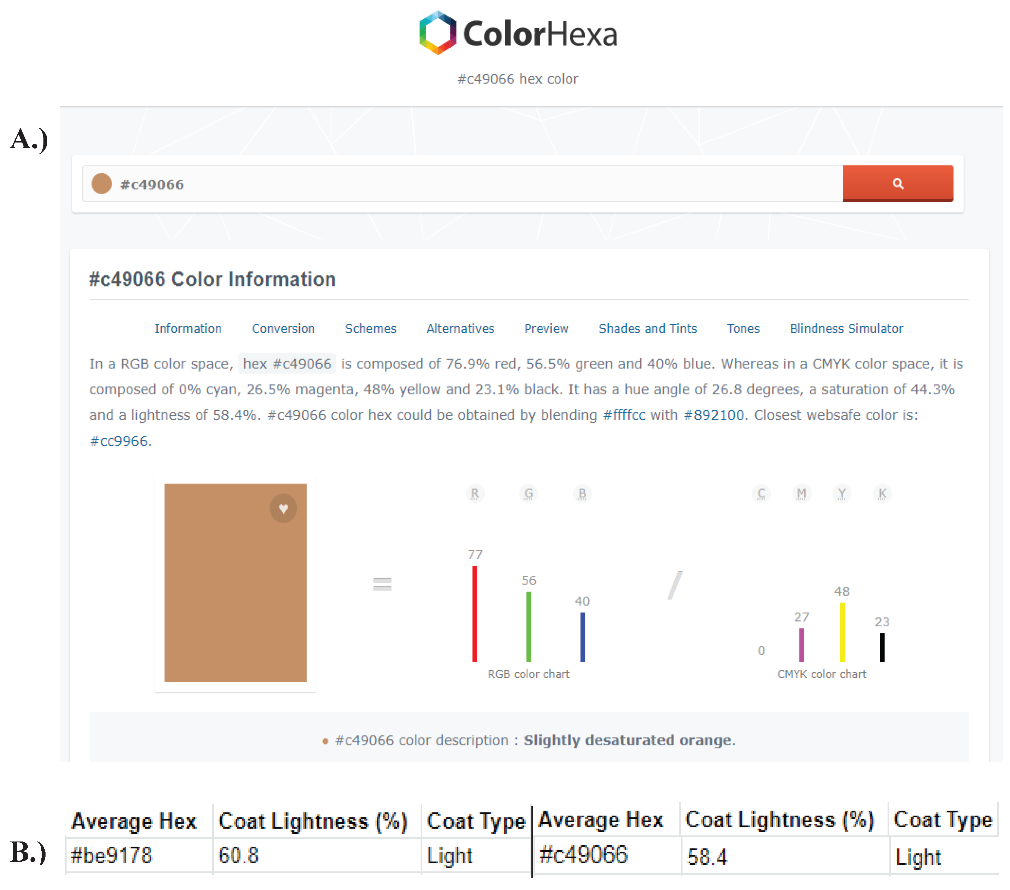
Figure A10. Determining the percentage lightness of hexadecimal codes. A.) To determine the ‘Percentage Coat Lightness’, and subsequent coat colour, the most recently obtained average hexadecimal code (e.g., #C49066) was inserted into the website found at: https://www.colorhexa.com/. This site provided the statistics of an input hexadecimal code, including the percentage lightness (e.g., 58.4%). B.) The new ‘Percentage Coat Lightness’ was entered into the spreadsheet, and the new ‘Coat Type’ was determined using a scale of percentages, obtained from each individual.

Figure A11. ‘Hexadecimal Information’ spreadsheet. The ‘Hex Info’ spreadsheet contained all data regarding the coat colour of giraffes on the Mogalakwena River Reserve. A. The main sheet consisted of the name of an individual, each hexadecimal code obtained via an image, the final average value, the percentage lightness corresponding to the final average code, and the colour group assigned to each percentage, for each individual B. The brown scale was used as a reference at the beginning of the work into giraffe coat colour. A scale called ‘Spot Colour via Percentile’ was created using the final average coat colour of each individual, allowing each member of the community to be placed into a coat colour group of either dark, medium, or light.

References

Andrade, D. V. , Gavira, R. S. B. and Tattersall, G. J. (2015) 'Thermogenesis in ectothermic vertebrates', Temperature (Austin), 2(4), pp. 454-454.
Berry, P.S.M.; Bercovitch, F.B. Darkening coat colour reveals life history and life expectancy of male Thornicroft's giraffes. J. Zoöl. 2012, 287, 157–160. [Google Scholar] [CrossRef]
Brand, R. 2007. Evolutionary Ecology of Giraffes (Giraffa camelopardalis) in Etosha National Park, Namibia. PhD Thesis. Newcastle University.
Cameron, E.Z.; du Toit, J.T. Social influences on vigilance behaviour in giraffes, Giraffa camelopardalis. Anim. Behav. 2005, 69, 1337–1344. [Google Scholar] [CrossRef]
Carnaby, T. 2008. Beat About the Bush: Birds. Johannesburg: Jacana Media.
Carlton, P. L. and Marks, R. A. (1958) 'Cold Exposure and Heat Reinforced Operant Behavior', Science (American Association for the Advancement of Science), 128(3335), pp. 1344-1344.
Carter, K.D.; Brand, R.; Carter, J.K.; Shorrocks, B.; Goldizen, A.W. Social networks, long-term associations and age-related sociability of wild giraffes. Anim. Behav. 2013, 86, 901–910. [Google Scholar] [CrossRef]
Castles, M.P.; Brand, R.; Carter, A.J.; Maron, M.; Carter, K.D.; Goldizen, A.W. Relationships between male giraffes’ colour, age and sociability. Anim. Behav. 2019, 157, 13–25. [Google Scholar] [CrossRef]
Crompton, A. W. , Taylor, C. R. and Jagger, J. A. (1978) 'Evolution of homeothermy in mammals', Nature (London), 272(5651), pp. 333-336.
Deacon, F.; Tutchings, A. The South African giraffeGiraffa camelopardalis giraffa: a conservation success story. Oryx 2018, 53, 45–48. [Google Scholar] [CrossRef]
Drevelle, M. 2019. The use of the giraffe’s neck in a thermoregulation behaviour. Internal MRC report. Unpublished.
Epstein, A. N. and Milestone, R. (1968) 'Showering as a Coolant for Rats Exposed to Heat', Science (American Association for the Advancement of Science), 160(3830), pp. 895-896.
Faure, O. , 2010. An ecological study of the vegetation and animal population dynamics of the Mogalakwena Reserve (S 22°43‟32”, E 028°46‟31”), Limpopo Province, s.l.: Mogalakwena Research Centre.
Fennessy, J.; Bidon, T.; Reuss, F.; Kumar, V.; Elkan, P.; Nilsson, M.A.; Vamberger, M.; Fritz, U.; Janke, A. Multi-locus Analyses Reveal Four Giraffe Species Instead of One. Curr. Biol. 2016, 26, 2543–2549. [Google Scholar] [CrossRef] [PubMed]
Giraffe Conservation Foundation. 2022. SOUTHERN GIRAFFE Giraffe Species. Available at: https://giraffeconservation.org/giraffe-species/southern/ [Accessed: ]. 12 January.
Girard, G. 2019. The importance of shade, coat colour and neck use in giraffe thermoregulation. Internal MRC report. Unpublished.
Htonl. 2016. Location in Limpopo. Available at: https://en.wikipedia.org/wiki/Mogalakwena_Local_Municipality#/media/File:Map_of_Limpopo_with_Mogalakwena_highlighted_(2016).svg [Accessed: ]. 6 February.
Jain, S.; Jain, P. The rise of Renewable Energy implementation in South Africa. Energy Procedia 2017, 143, 721–726. [Google Scholar] [CrossRef]
Jessen, C. Thermal afferents in the control of body temperature. Pharmacol. Ther. 1985, 28, 107–134. [Google Scholar] [CrossRef] [PubMed]
Kuntsch, V. and Nel, J. A. J. 1990. Possible thermoregulatory behaviour in Giraffa camelopardalis. Mammalian Biology. 55, 60-62. Available at: https://www.zobodat.at/pdf/Zeitschrift-Saeugetierkunde_55_0060-0062.pdf [Accessed: ]. 05 April.
Macé, B. 2021. Shade use and foraging strategy as behavioural thermoregulation traits in South African giraffes. Internal MRC report. Unpublished.
Mitchell, G.; Skinner, J. Giraffe Thermoregulation: a review. Trans. R. Soc. South Afr. 2004, 59, 109–118. [Google Scholar] [CrossRef]
Mitchell, G.; van Sittert, S.; Roberts, D.; Mitchell, D. Body surface area and thermoregulation in giraffes. J. Arid. Environ. 2017, 145, 35–42. [Google Scholar] [CrossRef]
Mogalakwena Research Centre. 2021. Whatsapp Message to R. Masterman 15 November.
Mogalakwena Research Centre. 2022. Email to R.
Mucina, L. and Rutherford, M., 2006. The vegetation of South Africa, Lesotho and Swaziland. Pretoria: Strelitzia 19 South African National Biodiversity Institute.
Muller, Z. et al. 2018. Giraffe Giraffa camelopardalis. Available at: https://www.iucnredlist.org/species/9194/136266699#assessment-information [Accessed: ]. 7 January.
Nakamura, K.; Morrison, S.F. A thermosensory pathway that controls body temperature. Nat. Neurosci. 2007, 11, 62–71. [Google Scholar] [CrossRef] [PubMed]
Nakamura, K.; Morrison, S.F. A thermosensory pathway mediating heat-defense responses. Proc. Natl. Acad. Sci. 2010, 107, 8848–8853. [Google Scholar] [CrossRef]
Osilla, E. V. , Marsidi, J. L., Sharma, S. 2021. Physiology, Temperature Regulation. In Statpearls. Treasure Island: Statpearls Publishing.
Polymeropoulos, E. T. , Oelkrug, R. and Jastroch, M. (2018) 'Editorial: The Evolution of Endothermy–From Patterns to Mechanisms', Frontiers in Physiology, 9.
Samsung Electronics. [no date]. Specifications. Available at: https://www.samsung.com/global/galaxy/galaxy-s10/specs/ [Accessed ]. 12 February.
Scholes, R. J. and Archer, S. R. (1997) 'Tree-grass interactions in savannas', Annual review of ecology and systematics, 28(1), pp. 517-544.
Stander. 2021. Email To R. Masterman 22 November.
Stuart-Fox, D.; Newton, E.; Clusella-Trullas, S. Thermal consequences of colour and near-infrared reflectance. Philos. Trans. R. Soc. B: Biol. Sci. 2017, 372, 20160345. [Google Scholar] [CrossRef] [PubMed]
Takealot Online (Pty) Ltd. [no date]. Digital Temperature & Humidity Thermometer Indoor Clock. Available at: https://www.takealot.com/digital-temperature-humidity-thermometer-indoor-clock/PLID51943043/description [Accessed: ]. 12 February.
Tan, C.L.; Knight, Z.A. Regulation of Body Temperature by the Nervous System. Neuron 2018, 98, 31–48. [Google Scholar] [CrossRef] [PubMed]
Tansey, E. A. and Johnson, C. D. (2015) 'Recent advances in thermoregulation', Advances in physiology education, 39(3), pp. 139-148.
TUBS. 2011. Location of Limpopo in South Africa. Available at: https://en.wikipedia.org/wiki/Limpopo#/media/File:Limpopo_in_South_Africa.svg [Accessed: ]. 6 February.
Winter, S.; Fennessy, J.; Janke, A. Limited introgression supports division of giraffe into four species. Ecol. Evol. 2018, 8, 10156–10165. [Google Scholar] [CrossRef] [PubMed]
Woolston, C. (2016) 'DNA reveals that giraffes are four species-not one', Nature (London), 537(7620), pp. 290-291.

Figure 1. Average monthly maximum and minimum temperatures between September 2019 - June 2022. Temperature is indicated with percentage deviation, as represented by vertical bars. The highest average maximum temperatures are observed annually between December and February, with a maximum monthly average recorded in November 2021, at 40.2°C. The lowest minimum average temperatures are observed annually between June and August, with a minimum monthly average recorded in August 2020, at 9.1°C. A trend of decreasing annual temperatures has been observed across temperature collection, as represented by decreasing graduated trend lines.

Figure 2. Linear regression for significant positions as a function of maximum daily air temperature. Each plot displays the trend for a Relative Position Duration, found to be significant through a Spearman correlation against the maximum daily air temperature. A.) The relative time per focal facing the sun is plotted as a function of maximum temperature. B.) The relative time per focal facing directly away from the sun is plotted as a function of maximum temperature. C.) The relative time per focal facing partially away from the sun is plotted as a function of maximum temperature.

Figure 3. Boxplots for relative time spent facing the sun among three age categories. The percentage proportions of each 15-minute focal spent facing the sun were divided into the Adult, Juvenile, and Sub-Adult age categories.

Figure 4. Boxplot visualisation of Relative Time Facing the Sun against Sex.

Figure 5. Boxplot visualisation of Relative Time Facing the Sun against coat colour.

Figure 6. Significant regression plot for the proportion of each focal fully exposed as a function of maximum temperature. The percentage proportion of each 15-minute focal session in any given exposure (Full, None, Partial) was plotted against the maximum daily air temperature, using a trendline to visualise correlation. Only significant plots were reported.

Figure 7. Boxplot visualisation of Relative Time Facing the Sun against season.

Table 1. Results of Spearman Correlation between maximum daily air temperature and Relative Position Duration. The Relative Position Duration (arb. unit) is divided into three positions: towards, away, and partially away from the sun. These are correlated against maximum daily air temperature. The values for S, ρ, and p are recorded in the table; significant p-values are marked with an ‘*’.

	Maximum Temperature
		S	p	p-value
Relative Position Duration	Towards	13231004	0.31	<0.01*
	Away	35391291	0.19	<0.01*
	Partially away	248012875	-0.36	<0.01*

Table 2. Reported values for the Shapiro-Wilk, Levene’s and Kruskal-Wallis tests on the Relative Time Facing the Sun against age. Values for normality, equality of variance, and independence of groups signify that a Kruskal-Wallis test is required to test for significance between Relative Time Facing the Sun and age. A significant difference between age and Relative Time Facing the Sun was detected (p-value ≤0.05).

	Shapiro-Wilk p-value	Levene’s Test p-value	Kruskal-Wallis Test
	Juvenile Sub-Adult Adult		χ2 Df p-value
Relative Time Facing Sun	<0.01 <0.01 <0.01	0.02	13.35 2 <0.01*

Table 3. Reported Z and p-values for a Dunn test comparing three separate age categories. The Z-value result of the test displays the direction of the trend, with a positive value denoting a positive trend, and a negative value denoting a negative trend. Adjusted p-values show where significance occurs, between each combination of age groups, with significant results marked with ‘*’ (p-value ≤0.05).

Comparison	Z	Adjusted p-value
Adult – Juvenile Adult – Sub-Adult Juvenile – Sub-Adult	2.70 -2.11 -3.52	0.02* 0.10 <0.01*

Table 4. Reported values for the Shapiro-Wilk, Levene’s and Wilcoxon-Mann-Whitney tests for Relative Time Facing the Sun and sex. The normality of variables was determined by a Shapiro-Wilk test, with p≤0.05 representing non-normal data. The equality of variance was determined with a Levene’s test, with p≤0.05 displaying unequal variance among the data. The Significance was tested using a Wilcoxon-Mann-Whitney test, with significance being identified by p≤0.05 (‘*’).

	Shapiro-Wilk p-value	Levene’s Test p-value	Wilcoxon-Mann-Whitney p-value
	Male Female
Relative Time Facing Sun	<0.01 <0.01	<0.01	0.01*

Table 5. Reported values for the Shapiro-Wilk, Levene’s and Kruskal-Wallis tests on Relative Time Facing the Sun against coat colour. Values for normality, equality of variance, and independence of groups signify that a Kruskal-Wallis test is required to test for significance between Relative Time Facing the Sun and coat colour. A significant difference between coat colour and Relative Time Facing the Sun was detected (p-value ≤0.05).

	Shapiro-Wilk p-value	Levene’s Test p-value	Kruskal-Wallis Test
	Dark Medium Light		χ2 Df p-value
Relative Time Facing Sun	<0.01 <0.01 <0.01	<0.01	261.17 72 <0.01*

Table 6. Reported values for a Dunn test between coat colour and Relative Time Facing the Sun.

Comparison	Z	Adjusted p-value
Dark - Light Dark - Medium Light - Medium	3.26 -0.96 -4.06	<0.01* 0.34 <0.01*

Table 7. Reported values for the Spearman correlation between Relative Exposures per Focal and the maximum temperature. The relative time spent in each exposure per 15-minute session was divided into Full, Partial, and No exposure. The S, ρ, and p values of the correlation are displayed in the table, with significant p-values denoted by ‘*’.

	Maximum Temperature
	Exposure	S	ϱ	p-value
Relative Exposure per Focal	Full None Partial	4029771 47888 969382	0.16 <0.01 <0.05	<0.01* 1.00 0.52

Table 8. Reported values for the Shapiro-Wilk, Levene’s and Wilcoxon-Mann-Whitney tests for Relative Time Facing the Sun against season. The normality of variables was determined by a Shapiro-Wilk test, with p≤0.05 representing abnormally distributed data. The equality of variance was determined with a Levene’s test, with p≤0.05 displaying unequal variance amongst the data. The significance was tested using a Wilcoxon-Mann-Whitney test, with significance being identified by p≤0.05 (‘*’).

	Shapiro-Wilk p-value	Levene’s Test p-value	Wilcoxon-Mann-Whitney p-value
	Dry Wet
Relative Time Facing Sun	<0.01 <0.01	<0.01	0.01*

Disclaimer/Publisher’s Note: The statements, opinions and data contained in all publications are solely those of the individual author(s) and contributor(s) and not of MDPI and/or the editor(s). MDPI and/or the editor(s) disclaim responsibility for any injury to people or property resulting from any ideas, methods, instructions or products referred to in the content.

© 2024 by the author. Licensee MDPI, Basel, Switzerland. This article is an open access article distributed under the terms and conditions of the Creative Commons Attribution (CC BY) license (https://creativecommons.org/licenses/by/4.0/).

Copyright: This open access article is published under a Creative Commons CC BY 4.0 license, which permit the free download, distribution, and reuse, provided that the author and preprint are cited in any reuse.

MDPI Initiatives

Important Links

Choose an area of interest and we will send you notifications of new preprints at your preferred frequency.

Disclaimer

Analysis of Behavioural Thermoregulatory Responses in Giraffa, Regarding Temperature and Sunlight Exposure during Daylight Hours

Abstract

1. Introduction

2. Materials and Methods

2.1. Study Area

2.2. Study Group

2.3. Data Collection

2.4. Data Analysis

3. Results

3.1. Relationship between Temperature and Time Spent Facing the Sun

3.2. Relationship between Age and Time Spent Facing the Sun

3.3. Relationship between Sex and Time Spent Facing the Sun

3.4. Relationship between Coat Colour and Time Spent Facing the Sun

3.5. Relationship between Temperature and Shade Usage

3.6. Relationship between Seasons and Time Spent Facing the Sun

4. Discussion

5. Conclusions

Funding

Data Availability Statement

Acknowledgments

Conflicts of Interest

Appendix A

References

MDPI Initiatives

Important Links

Subscribe