Preprint
Article

Cost Effectiveness Analysis of Optimal Rabies Control Strategies

Altmetrics

Downloads

170

Views

76

Comments

0

Submitted:

27 March 2024

Posted:

28 March 2024

You are already at the latest version

Alerts
Abstract
A mathematical model that incorporates human attacks on dogs is presented to explore the dynamics of rabies transmission. The model divided the infection rate into two categories: dog-to-dog transmission rates during the prodromal phase (βdP) and the furious phase (βdF). It has been determined that the model is well-posed and that all of the solutions are positive, as well as the feasibility and positivity of the model's solutions. Both the basic reproduction number (R0) and the effective reproductive number (Re) are computed, and it is demonstrated that the model has a unique disease-free equilibrium that is globally asymptotically stable whenever Re < 1. To identify the model's most sensitive parameters and the ones that intervention efforts should focus on, sensitivity analysis of the effective reproduction number is carried out. We can construct an optimal control system using the state equations, the adjoint equations, and the optimality condition that determines the controls by applying Pontryagin's Maximum/Minimum principle. To help decision-makers in allocating funds for rabies interventions, cost-effectiveness analyses are conducted. To determine the degree to which the intervention strategies are advantageous and cost-effective, this study performs a cost-effective analysis of one or all possible combinations of the optimal rabies control strategies (pre-exposed and post-exposed vaccination for both dog and human populations) for the four different transmission settings. After arranging the techniques to increase effectiveness (total infections prevented), a cost-effective analysis using the Incremental Cost Effectiveness Ratio (ICER) was conducted. The result supports the function that the four intervention options are performing to either completely eradicate or significantly reduce rabies disease among the populations. The dynamical behavior of the system is studied through simulations using the ode45 numerical technique from MATLAB.
Keywords: 
Subject: Computer Science and Mathematics  -   Mathematical and Computational Biology

1. Introduction

Rabies is a zoonotic disease that affects Ethiopia’s livestock industry and public health, according to Abera et al. (2024). The burden and distribution of rabies in the country on both humans and animals were researched. By gathering data from the Ethiopian Public Health Institute (EPHI) and the Ministry of Agriculture over five years (2018–2022), the authors carried out an in-depth descriptive analysis of rabies. They showed a higher prevalence and broader spread of rabies throughout the country in humans as well as animals. The results account for the increasing number of suspected cases of human rabies exposure and mortality as animal outbreaks continue to spread. The animal species most frequently impacted were dogs, then camels, cattle, and horses.
Ruan Shigui (2017), Created a simple susceptible, exposed, infectious, and recovered (SEIR) type model to represent the transmission of the rabies virus from dogs to humans as well as between dogs and other dogs. The constructed model was used to reproduce data on human rabies cases in China from 1996 to 2010. Following that, the author included both domestic and stray dogs in the basic model and used it to mimic human rabies data from Guangdong Province, China. Furthermore, from January 2004 to December 2010, the Chinese Ministry of Health released monthly data on human rabies cases. He used this data and created an SEIR model with periodic transmission rates. With the system of ordinary differential equations, Musaili and Chepkwony (2020) updated the SIR model of infectious diseases to take into consideration the transmission of the rabies virus in dogs and included public health education as a control mechanism. They identified the equilibrium points for both endemic and disease-free conditions by computing the reproduction number. An SEIR and SEIV model was presented by Eze et al. (2020) to explain the dynamics of rabies virus transmission in humans and dogs. They computed the disease-free and endemic equilibrium points, as well as the basic reproduction number. They also obtained a control solution for the model, which predicts that increasing pre-exposure prophylaxis in humans and dogs as well as public education help eliminate rabies-related deaths. However, the results indicated that, if complete eradication of the disease is desired, pre- and post-exposure prophylaxis in humans along with vaccination in the dog population. Any combined approach that includes vaccinating the dog population increases the disease’s ability to be eradicated. A mathematical model that represented the dynamics of the rabies virus transmission between dogs and human beings was developed by Thongtha and Modnak (2021). They also used optimal control theory and equilibrium state analysis to try to minimize the cost of rabies vaccinations. A mathematical model was developed by Pantha et al. (2021) to explain the dynamics of rabies transmission in Nepal. Researchers can properly estimate parameters associated with rabies transmission in Nepal, which makes use of annual dog-bite data which was obtained from Nepal over ten years. They discovered that the main factors influencing the number of reproductions are dog-related elements. The findings suggest that jackals might have contributed to the ongoing epidemic of rabies in Nepal, although to a smaller degree than dogs. Additionally, based on the model, control measures significantly decrease the number of cases, though jackal vaccinations are unlikely to be as successful as dog-related preventative measures.
Motivation for the present work
The majority of studies in the literature mainly focused on developing SEIR models for both dog and human populations. In general, SEIR models of dogs assume that the cause of death for all infected dogs is rabies disease. However, medical literature reported that the behavior of rabies in the infected class is not constant but differed linearly. That is, the infected class is divided into three phases: (i) prodromal (ii) furious, and (iii) paralytic [21]. In the first phase i.e., prodromal phase dogs become shy and seek out isolated areas. In the second phase i.e., furious phase dogs become extremely irritable and aggressive. In the end phase or third phase i.e., the paralysis phase dogs lose their capacity to move normally, chew, and swallow.
Here, it is clear that the rrabies-infecteddog’s behavior is not the same always but differs linearly with time. The nature of the rabies disease we intend to include in the current study. In this study, the infected compartment is divided into (i) the prodromal phase and (ii) the furious phase compartments. However, the paralysis phase is omitted from consideration. This is because the dogs in this phase are highly inactive. That is, these paralytic dogs cannot move from one place to another place and therefore they can rarely transmit the disease.
However, it is assumed that rabies only causes mortality among dogs in the furious phase rather than the prodromal phase and the model divided the infection rate into two categories: dog-to-dog transmission rates during the prodromal phase ( β d P ) and the furious phase ( β d F ).
Furthermore, the human population is divided into SEIR compartmental structures. Unlike infected dogs, infected humans do not transmit the disease to others. Hence, in the case of humans splitting of infected class is not meaningful. Hence, the infected human class is left without splitting in this study.
This investigation is motivated by therefore mentioned considerations and is aimed to address these gaps.
In Section 2, the model assumptions are listed. State variables and model parameters are described and presented in tabular forms. A model flowchart is also included. A model consisting of nine compartments is developed: (i) five compartments structure   S d E d I d P I d F R d   is for the dog population and (ii) four compartments structure S h E h I h R h   is for the human population.
Section 3: defines the model’s boundedness and positivity, as well as equilibrium points of the model are determined. Both the basic reproductive number (R0) and the effective reproductive number (Re) are computed using the next-generation matrix approach. It shows that the disease-free equilibrium (DFE) is globally stable.
Section 4: The sensitivity analysis and Interpretation of Sensitivity Indices presented in the figures show the numerical simulation of the relationship between the sensitive parameters and the effective reproductive number.
Section 5: Pontryagin’s Maximum Principle is applied and the fundamentals of optimal control are examined.
Section 6: the simulation results are presented. The rate of per-exposed and post-exposed vaccination for both populations are considered as control mechanisms.
Section 7: A cost-effective analysis using the Incremental Cost Effectiveness Ratio (ICER) was conducted. Population dynamics are demonstrated through graphs.
The paper ends in Section 8 with recommendations and conclusions.

2. Description and Model Formulation

Here, a system of continuous nonlinear deterministic ordinary differential equations is used to create a mathematical model. The main objective of this model is to evaluate the way per-exposure and post-exposure vaccinations are effective rabies control methods for both dogs and humans. The dog and the human model are the two subpopulations that are involved in the spread of the rabies virus. The dog population is divided into five compartments: (i) susceptible dogs   S d (ii) exposed dogs E d (iii) infected dogs in the prodromal phase I d P (iv) infected dogs in the furious phase I d F (v) recovered dogs R d due to pre-exposure vaccination. This S d E d I d P I d F R d   dog model is an extension of the existing SEIR model used to describe the dynamics of dog rabies.
Similarly, the human population is divided into four compartments consisting of (i) susceptible humans S h (ii) exposed humans   E h (iii) infected humans I h , and (iv) recovered humans R h due to post-exposure vaccination.
Both susceptible dogs and susceptible human individuals are at risk of catching the disease from rabid dogs. Both exposed dogs and humans have been exposed to the virus but they do not yet show any symptoms. That is, at this stage, they are not capable of transferring the disease.
Infected individuals, both dogs and humans, are unlikely to recover from rabies. If the exposed humans are immunized or given treatment before they become infectious then they will recover from the disease.
The model includes nine ordinary differential equations and is based on the following assumptions:
  • Susceptible populations of dogs and humans are recruited at a rate level A d   a n d   A h .
  • The rabies infection does not transfer from infected humans to susceptible dogs.
  • Rabies transmission from humans to humans was ignored.
  • Exposed dogs cannot transfer the rabies disease either to dogs or to humans.
  • Giving post-exposed prophylaxis for dogs and humans.
  • Giving pre-exposed prophylaxis for dogs and humans.
  • For dogs, giving both pre-exposed and post-exposure treatment or prophylaxis.
  • The primary way of rabies virus transmission is (i) from infectious dogs to susceptible dogs and (ii) from infectious dogs to susceptible humans.
  • Individuals in each compartment have an equal natural death rate.
  • All the model parameters are positive quantities.
Based on the aforementioned assumptions, the dynamics of the disease in both dog and human populations are demonstrated through a flowchart and are shown in Figure 1.
2.1. Model Equations
The ordinary differential equation below illustrates the paths of infection based on the transmission model shown in Figure 1.
  d S d d t = A d β d P I d P + β d F I d F S d μ d + v d S d   + α d R d     d E d d t = ( β d P I d p + β d F I d F ) S d μ d + δ d + θ d E d   d I d p d t = δ d E d μ d + ρ d + c d I d P   d I d F d t = ρ d I d P μ d + ε d + c d I d F   d R d d t = v d S d + θ d E d μ d + α d R d     d S h d t = A h ( β h P I d P + β h F I d F ) S h μ h + v h S h + α h R h   d E h d t = ( β h P I d P + β h F I d F ) S h μ h + δ h + θ h E h   d I h d t = δ h E h μ h + ε h I h     d R h d t = v h S h + θ h E h μ h + α h R h  
Table 1. Description of variables and parameters of the system (1).
Variables and Parameters Description
S d
E d
I d p
I d F
R d
S h
E h
I h
R h
A d
β d P
β d F
δ d
ρ d
v d
θ d
ε d
μ d
α d
A h
β h P
β h F
δ h
v h
θ h
ε h
μ h
α h
Susceptible dog populations
Exposed dog population
Infectious dog population with prodromal phase
Infectious dog population with the furious phase
Recovered dog population
Susceptible human populations
Exposed human populations
Infectious human populations
Recovered human population
Dogs annual crop of newborn puppies
Prodromal phase dog -to-dog transmission rate
Furious phase dog-to-dog transmission rate
The incubation period of dog populations
Rate of prodromal to furious stage
Pre-exposure prophylaxis (vaccine) for dogs
Post-exposure prophylaxis (treatment) for dogs
The death rate of dogs due to rabies
The natural death rate of dogs
Loss of immunity in dogs
Human annual birth
Prodromal phase dog-to-human transmission rate
Furious phase dog -to-Human transmission rate
The incubation period of human populations
Pre-exposure prophylaxis (vaccine) for humans
Post-exposure prophylaxis (treatment) for humans
The death rate of humans due to rabies
Natural death rate of humans
Rate of recovery to Susceptible human

3. Model Analysis

3.1. Positivity

In this subsection, we show that the solutions of the system of model equations (1) are positive. This is stated in the form of a theorem accompanied by proofs
Positivity of dog population
Theorem 1:
Every solution of the system of model equations representing dog populations given in (1) together with the initial conditions exists in the interval [ 0 , ) . Also, the solutions are positive.
Proof: 
Here we show that the solutions for the dog population equations given in model system (1) exist Also, we show that they are non-negative i.e., S d t > 0 ,   E d t 0 ,   I d P t 0 ,   I d F t 0 ,   R d t 0 . That is, if the initial conditions S d 0 ,   E d 0 ,   I d P 0 ,   I d F 0 ,   R d 0 are non-negative then so are the variables S d t ,   E d t ,   I d P t ,   I d F t ,   R d t for all t 0 .
The solutions S d t ,   E d t ,   I d P t ,   I d F t ,   R d t of the system (1) together with the initial conditions exits and unique on [ 0 , k ) where 0 < k < +   since the right-hand side of the system is completely continuous and locally Lipshitzian on C .
We now consider the dog population equations given in (1), one by one, and show that the solutions of the dog variables are non-negative i.e., S d t > 0 ,   E d t 0 ,   I d P t 0 ,   I d F t 0 ,   R d t 0 for all t 0 .
Positivity of susceptible dog population: Consider the model equation for susceptible dog population d S d / d t = A d β d P I d p + β d F I d F S d μ d + v d S d + α d R d . It can be expressed without loss of generality, after elimination of the positive term A d   which appears on the right-hand side, as an inequality as d S d / d t β d P I d p + β d F I d F S d μ d + v d S d .This inequality can also be expressed as   d S d / S d π 1 d t . Here, the function π 1   denoting the expression π 1 = β d P I d p + β d F I d F μ d + v d   can be negative zero or positive valued. Now, using the variables separation method and upon integrating, the solution of d S d / S d π 1 d t   can be obtained as S d t S d 0   e π 1 d t .   Here, the integral constant S d 0   is the initial susceptible dog population and is assumed to be a non-negative quantity S d 0 0 . Similarly, an exponential function is always a non-negative quantity irrespective of the value of the exponent i.e., e π 1 d t 0 . Hence, we conclude that   S d t 0 . That is, the susceptible dog population size is a positive quantity.
Positivity of exposed dog population: Consider the model equation for exposed dog population d E d / d t μ d + δ d + θ d E d . Alternately, it can be expressed as d E d / E d π 2 d t . Here, the function π 2 denoting the expression π 2 = μ d + δ d + θ d   can be negative zero or positive valued. Now, using the variables separation method and applying integration, the solution of   d E d / E d π 2 d t   can be obtained as E d t = E d 0   e π 2 d t . Here, the integral constant E d 0   is the initial population of exposed dogs and is assumed to be a non-negative quantity E d 0 0 . Similarly, an exponential function is always a non-negative quantity irrespective of the value of the exponent i.e., e π 2 d t 0 . Hence, we conclude that E d t 0 . That is, the exposed dog population size is a positive quantity.
Positivity of Infectious dog population in prodromal phase: Consider the model equation for prodromal dog population   d I d p / d t = δ d E d μ d + ρ d + c d I d P . Here, the term   δ d E d   is a positive quantity since   δ d   is a positive parameter and the exposed dog population   E d is already shown positive. Now, the aforementioned ODE can be expressed without loss of generality, after eliminating the positive term   δ d E d , as an inequality as   d I d p / d t μ d + ρ d + c d I d P . Now, using the variables separation method and integrating, the solution can be obtained as I d p t = I d p 0   e μ d + ρ d + c d   d t . Here, the integral constant I d p 0   is the initial population of prodromal infectious dogs and is assumed to be a non-negative quantity I d p 0 0 . Similarly, the exponential term is also a positive quantity i.e., e μ d + ρ d + c d   d t   0   since the integrand in the exponent consists of positive parameters only. Hence, we conclude that   I d p t 0 . That is, the prodromal infectious dog population size is a positive quantity.
Positivity of Infectious dog population in furious phase: Consider the model equation for infectious dog population in furious phase   d I d F / d t = ρ d I d P μ d + ε d + c d I d F . Here, the term ρ d I d P   is positive since ρ d   is a positive parameter and the prodromal infectious dog population   I d P is already shown positive. Now, the aforementioned ODE can be expressed without loss of generality, after eliminating the positive term   ρ d I d P , as an inequality as   d I d F / d t μ d + ε d + c d I d F . Now, using the variables separation method and integrating, the solution can be obtained as I d F t I d F 0   e μ d + ε d + c d   d t . Here, the integral constant I d F 0   is the initial population of furious infectious dogs and is assumed to be a non-negative quantity I d F 0 0 . Similarly, the exponential term is also positive i.e., e μ d + ε d + c d   d t   0   since the integrand in the exponent consists of positive parameters only. Hence, we conclude that   I d F t 0 . That is, the furious infectious dog population size is a positive quantity.
Positivity of Recovered Dog Population: Consider the model equation for the recovered dog population as   d R d / d t = v d S d + θ d E d μ d + α d R d . Here, the term s   v d S d and θ d E d are positive since θ d   and v d are positive parameters and the susceptible and Exposed dog population s   are already shown positive. Now, the aforementioned ODE can be expressed without loss of generality, after eliminating the positive terms   v d S d , θ d E d ,   as an inequality as   d R d / d t μ d + α d R d . Now, using the variables separation method and integrating, the solution can be obtained as R d   t R d   0   e μ d + α d   d t . Here, the integral constant R d 0   is the initial population of recovered dogs and is assumed to be a non-negative quantity R d 0 0 . Similarly, the exponential term is also positive i.e., e μ d + α d   d t   0   since the integrand in the exponent consists of positive parameters only. Hence, we conclude that   R d t 0 . That is, the recovered dog population size is a positive quantity.
Positivity of the human population
Theorem 2:
Every solution of the system of model equations representing human populations given in (1) together with the initial conditions exists in the interval [ 0 , ) . Also, the solutions are positive.
Proof: 
Here we show that the solutions for the human population equations given in model system (1) exist. Also, we show that they are non-negative i.e., S h t 0 ,   E h t 0 ,   I h t 0 ,   R h t 0 . That is, If the initial conditions S h 0 ,   E h 0 ,   I h 0 ,   a n d   R h 0 are non-negative then so are the variables S h t ,   E h t ,   I h t ,   R h t for all t 0 .
The solutions S h t ,   E h t ,   I h t ,   R h t of the system (1) together with the initial conditions exits and unique on [ 0 , k ) where 0 < k < +   since the right-hand side of the system is completely continuous and locally Lipshitzian on C .
We now consider the human population equations given in (1), one by one, and show that the solutions of the human variables are non-negative i.e., S h t 0 ,   E h t 0 ,   I h t 0 ,   R h t 0 for all t 0 .
Positivity of susceptible human population: Consider the model equation for susceptible human population   d S h / d t =   A h β h I d p + I d F S h ( μ h + v h ) S h + α h R h . It can be expressed without loss of generality, after eliminating the positive term A h   appearing on the right-hand side, as an inequality as d S h / d t β h P I d p + β h F I d F S h ( μ h + v h ) S h . This inequality can also be expressed as   d S h / S h Q 1 d t . Here, the function Q 1   denoting the expression Q 1 = β h P I d p + β h F I d F ( μ h + v h )   can be negative or zero or positive valued. Now, using the variables separation method and upon integrating, the solution can be obtained as S h t S h 0   e Q 1 d t .   Here, the integral constant S h 0   is the initial susceptible human population and is assumed to be a non-negative quantity S h 0 0 . Similarly, an exponential function is always a non-negative quantity irrespective of the value of the exponent i.e., e Q 1 d t 0 . Hence, we conclude that   S h t 0 . That is, the susceptible human population size is a positive quantity.
Positivity of exposed human population: Consider the model equation for exposed human population d E h / d t μ h + δ h + θ h E h .
Alternately, it can be expressed as   d E h / E h Q 2 d t . Here, the function Q 2   denoting the expression Q 2 = μ h + δ h + θ h   can be negative zero or positive valued. Now, using the variables separation method and applying integration, the solution can be obtained as E h t = E h 0   e Q 2 d t . Here, the integral constant E h 0   is the initial population of exposed humans and is assumed to be a non-negative quantity E h 0 0 . Similarly, an exponential function is always a non-negative quantity irrespective of the value of the exponent i.e., e Q 2 d t 0 . Hence, we conclude that   E h t 0 . That is, the exposed human population size is a positive quantity.
Positivity of Infectious human population: Consider the model equation for the infectious human population   d I h / d t = δ h E h μ h + ε h I h . Here, the term δ h E h   is a positive quantity since δ h   is a positive parameter and the exposed human population   E h is already shown positive. Now, the aforementioned ODE can be expressed without loss of generality, after eliminating the positive term   δ h E h , as an inequality as   d I h / d t μ h + ε h I h . Now, using the variables separation method and integrating, the solution can be obtained as I h t I h 0   e μ h + ε h   d t . Here, the integral constant I h 0   is the initial population of infectious humans and is assumed to be a non-negative quantity   I h 0 0 . Similarly, the exponential term is also a positive quantity i.e., e μ h + ε h   d t   0   since the integrand in the exponent consists of positive parameters only. Hence, we conclude that   I h t 0 . That is, the infectious human population size is a positive quantity.
Positivity of Recovered human population: Consider the model equation for the recovered dog population as   d R h / d t = v h S h + θ h E h μ h + α h R h . Here, the terms v h S h and   θ h E h   are positive since v h ,   a n d   θ h   are positive parameters and the susceptible and exposed human population are already shown positive. Now, the aforementioned ODE can be expressed without loss of generality, after eliminating the positive terms v h S h ,   θ h E h as an inequality as   d R h / d t μ h + α h R h . Now, using the variables separation method and integrating, the solution can be obtained as R h   t R h   0   e μ h + α h   d t . Here, the integral constant R h 0   is the initial population of recovered humans and is assumed to be a non-negative quantity i.e., R h 0 0 . Similarly, the exponential term is also positive i.e., e μ h + α h   d t   0   since the integrand in the exponent consists of positive parameters only. Hence, we conclude that   R h t 0 . That is, the recovered human population size is a positive quantity.
Theorem 3:
The feasible region Ω defined by Ω = Ω d x Ω h R + 5 x R + 4 is bounded.
Here,
Ω d = S d t , E d t , I d P t , I d F t , R d t R + 5   :   N d t A d μ d   Ω h = S h t , E h t , I h t , R h t R + 4   :   N h t A h μ h  
Also, N d t = S d t + E d t + I d P t + I d F t + R d t   is the total dog population.
Similarly,   N h t = S h t + E h t + I h t + R h t   is the total human population.
Furthermore, the sets Ω , Ω d ,   and Ω h are all real-valued.
Proof: 
Here, we show that the model population is bounded.
That is, the dog population is bounded i.e., N d t A d μ d
Also, the human population is bounded i.e., N h t A h μ h

3.2. Boundedness of the Model

The dog population is bounded
We now show that if the total dog population size is given by N d t = S d t + E d t + I d P t + I d F t + R d t then   lim t N d t A d μ d . In other words, the total size of the dog population given in model system (1) is bounded above.
Consider that N d denotes the total dog population at any time t.
Therefore
N d = S d + E d + I d P + I d F + R d
Upon derivation of both sides of equation (2.1) concerning time, we obtain
d N d d t = d S d d t + d E d d t + d I d P d t + d I d F d t + d R d d t
Now, making use of the system (1) and substituting for the differential terms appearing on the right-hand side of (3.2), the equation reduces to the form as
d N d d t = A d μ d N d c d I d P ( c d + ε d ) I d F
Here, the terms c d I d P   and c d + ε d I d F   are positive since all the model parameters are assumed to be positive and all the model variables are proved to be positive. Hence, upon removing these two positive terms, the equation (3.3) can be expressed as an inequality
d N d d t + μ d N d A d
It is a first-order nonlinear ODE with constant coefficients and its solution is given by
N d A d μ d + N d 0 A d μ d e μ d t
As t in equation (3.4) the population size N d A d μ d which implies that 0 N d A d μ d , Thus the feasible solution set of the system equation of the model enters and remains in the region:
Ω d = S d , E d , I d P , I d F ,   R d : N d A d μ d R + 5
The human population is bounded
We now show that if the total human population size is given by N h t = S h t + E h t + I h t + R h t then   lim t N h t A h μ h . In other words, the total size of the human population given in model system (1) is bounded above. Consider that N h denotes the total human population at any time t.
Therefore,
N h = S h + E h + I h + R h
Upon derivation of both sides of equation (3.6) concerning time, we obtain
d N h d t = d S h d t + d E h d t + d I h d t + d R h d t
Now, making use of the system (1) and substituting for the differential terms appearing on the right-hand side of (3.7), the equation reduces to the form after algebraic simplifications as
d N h d t = A h μ h N h ε h I h
Here, the term ε h I h   is positive since all the model parameters are assumed to be positive and all the model variables are proved to be positive.
Hence, upon removing this negative term, the equation (3.8) can be expressed as an inequality as
d N h d t + μ h N h A h
It is a first-order nonlinear ODE with constant coefficients and its solution is given by
N d A h μ h + N h 0 A h μ h e μ h t
As t in equation (3.9) the population size N h A h μ h which implies that 0 N h A h μ h , Thus the feasible solution set of the system equation of the model enters and remains in the region:
Ω h = S h , E h , I h ,   R h : N h A h μ h R + 4
Therefore, from equations (3.5) and (3.10) the region Ω = Ω + 5 × Ω + 4 is positively invariant and the model (1) is well-posed or biologically and epidemiologically. The proof of Theorem 3. is complete.

3.4. Disease-Free Equilibrium E 0

To determine the disease-free equilibrium, E 0 for the basic model we consider a scenario where none of the compartments are affected by rabies infection, i.e., when E d = I d P = I d F = E h = I h = 0 , and the control parameters v d ,   θ d ,   v h ,   θ h are zero. We set the right-hand side of system (1) to zero, leading to the following outcome:
A d μ d S d = 0
A h μ h S h = 0
E 0 = ( s d 0 , s h 0 ) = A d μ d , A d μ d
To determine the disease-free equilibrium for the effective model is similar to the basic model but considering the parameters v d ,   θ d ,   v h ,   θ h are different from zero
  A d β d P I d P + β d F I d F S d μ d + v d S d   + α d R d = 0   v d S d + θ d E d μ d + α d R d = 0     A h β h P I d P + β h F I d F S h μ h + v h S h + α h R h = 0     v h S h + θ h E h μ h + α h R h = 0  
One (3.12) is algebraically manipulated, the disease-free-equilibrium point can be represented as
E e = S d e ,   E d e ,   I d P e ,   I d F e ,   R d e ,   S h e ,   E h e ,   I h e ,   R h e .
When we manipulate equation (3.12) algebraically, we get the disease-free equilibrium point for an effective model
E e = A d μ d + α d μ d μ d + α d + v d , 0 , 0 , 0 , A d v d μ d μ d + α d + v d , A h μ h + α h μ h μ h + α h + v h , 0 , 0 , A h v h μ h μ h + α h + v h

3.5. Basic Reproduction Number ( R 0 )

To determine the basic reproduction number ( R 0 .), we apply the next-generation matrix method [7]. We can obtain the matrices f i and V i   for the new infection terms and the remaining transfer terms, taking into consideration that our infected compartments are E d , I d P , I d F ,   E h , and   I h
    d E d d t = ( β d P I d p + β d F I d F ) S d μ d + δ d E d   d I d p d t = δ d E d μ d + ρ d I d P   d I d F d t = ρ d I d P μ d + ε d I d F     d E h d t = β h P I d P + β h F I d F S h μ h + δ h E h     d I h d t = δ h E h μ h + ε h I h  
From equation (3.14) take the vectors f i and V i
f i = β d ( I d p + I d F ) S d 0 0 β h I d p + I d F S h 0 &   V i = μ d + δ d E d μ d + ρ d I d P δ d E d μ d + ε d I d F ρ d I d P μ h + δ h E h μ h + ε h I h δ h E h
The Jacobian matrices f i and   V i   at disease-free equilibrium from equation (3.11), respectively, are given by
F = 0 0 0 0 0   β d P A d μ d 0 0 β h P   A h μ h 0   β d F A d μ d 0 0   β h F A h μ h 0 0 0 0 0 0 0 0 0 0 0
V = ( μ d + δ d ) δ d 0 0 0 0 μ d + ρ d ρ d 0 0 0 0 μ d + ε d 0 0 0 0 0 μ h + δ h δ h 0 0 0 0 μ h + ε h
Given matrix V, its inverse is given by
V 1 = 1 ( μ d + δ d ) 0 0 0 0 δ d ( μ d + δ d ) μ d + ρ d 1 μ d + ρ d 0 0 0 ρ d δ d μ d + ρ d ( μ d + δ d ) μ d + ε d ρ d μ d + ρ d μ d + ε d   1 μ d + ε d 0 0 0 0 0 1 μ h + δ h 0 0 0 0 δ h μ h + δ h μ d + ε d 1 μ d + ε d
Take F and   V 1 from equations (3.15) and (3.16), the symbol ρ F V 1 represents the dominant eigenvalue in magnitude, or spectral radius, of a matrix F V 1 , thus basic reproductive number defended by R 0 = ρ F V 1
As a result, the following gives the effective reproduction number:
R 0 = A d δ d ( β d P μ d + ε d + ρ d β d F ) μ d μ d + ρ d μ d + ε d ( μ d + δ d )

3.5.1. Effective Reproduction Number

The average number of diseases caused by a single infectious individual in a society when intervention techniques are implemented—in this case, vaccinations for humans and dogs both before and after exposure—is known as the effective reproduction number.
By using the same method as R 0 but taking into consideration vaccines for dogs and humans both before and after exposure, and culling of infected dogs i.e.,   θ d ,   θ h ,   v d , v h   c d 0 , the effective reproduction number R e of system (1) is calculated.   R e = ρ F V 1 is the spectral radius, or dominant eigenvalue, of F V 1 .
The Jacobian matrices F and V at effective disease-free equilibrium E e , respectively, are given by
F = 0 0 0 0 0 β d P A d μ d + α d μ d μ d + α d + v d 0 0 β h P A h μ h + α h μ h μ h + α h + v h 0 β d F A d μ d + α d μ d μ d + α d + v d 0 0 β h F A h μ h + α h μ h μ h + α h + v h 0 0 0 0 0 0 0 0 0 0 0
V = ( μ d + δ d + θ d ) δ d 0 0 0 0 μ d + ρ d + c d ρ d 0 0 0 0 μ d + ε d + c d 0 0 0 0 0 μ h + δ h + θ h δ h 0 0 0 0 μ h + ε h
The inverse of matrix V is given by
V 1 = 1 ( μ d + δ d + θ d ) δ d ( μ d + δ d + θ d ) μ d + ρ d + c d ρ d δ d μ d + ρ d + c d ( μ d + δ d + θ d ) μ d + ε d + c d 0 0 0 1 μ d + ρ d + c d ρ d μ d + ρ d + c d μ d + ε d + c d   0 0 0 0 1 μ d + ε d + c d 0 0
0 0 0 1 μ h + δ h + θ h δ h μ h + δ h + θ h μ d + ε d 0 0 0 0 1 μ d + ε d
The symbol ρ F V 1 represents the dominant eigenvalue in magnitude, or spectral radius, of a matrix F V 1 , and take F a n d V 1 from equation (3.18) and (3.19), thus effective reproductive number defend by R e = ρ F V 1 Therefore, the effective reproduction number is as follows:
R e = A d ( β d P μ d + ε d + c d + ρ d β d F ) δ d ( μ d + α d ) μ d μ d + v d + α d μ d + ρ d + c d μ d + ε d + c d ( μ d + δ d + θ d )
When we now replace the parameter values from Table 2 with the expression given in Equations (3.17) and (3.20) for the basic and effective reproductive numbers, we obtain the following results.
R 0 = A d δ d ( β d P μ d + ε d + ρ d β d F ) μ d μ d + ρ d μ d + ε d ( μ d + δ d ) = 2.74
The fact that the basic reproductive number R 0 is larger than one in the absence of any control measures indicates that the disease will keep spreading in the population.
R e = A d ( β d P μ d + ε d + c d + ρ d β d F ) δ d ( μ d + α d ) μ d μ d + v d + α d μ d + ρ d + c d μ d + ε d + c d ( μ d + δ d + θ d ) = 1.78
The effective reproductive number R e is larger than one given the current vaccination coverage, indicating that the disease is still present. This suggests that greater measures should be taken to prevent the spread of rabies.

3.6. Global Stability of Disease-Free Equilibrium Points

We used the method suggested by [7] to investigate the global stability of the disease-free equilibrium point of the system (1).
The structure of our model, as shown in system (1), is as follows.
d X d t = B 0 X X 0 + B 1 Y d Y d t = B 2 Y  
The classifications of susceptible and vaccinated individuals are represented by X R + m . Classes of exposed and infectious individuals are represented by Y R + n A vector at DFE point ε 0 of the vector length as X is represented by Using system (1) as an example, we define:
X = S d R d S h R h ,   Y = E d I d P I d F E d I h   and   X ε 0 = A d μ d + α d μ d μ d + α d + v d A d v d μ d μ d + α d + v d A h μ h + α h μ h μ h + α h + v h A h v h μ h μ h + α h + v h ,   X X 0 = S d A d μ d + α d μ d μ d + α d + v d R d A d v d μ d μ d + α d + v d S h A h μ h + α h μ h μ h + α h + v h R d A h v h μ h μ h + α h + v h
To confirm whether the disease-free equilibrium is globally stable, we have to show that:
i.
B0 should be a matrix whose eigenvalues are real and negative; and
ii.
Bz should be a Metzler matrix.
Using system (1) and the representation in 3.21 the first equation can be rewritten as shown below:
A d + α d R d β d P I d P + β d F I d F + μ d + v d S d v d S d + θ d E d μ d + α d R d A h + α h R h ( β h P I d P + β h F I d F + μ h + v h ) S h v h S h + θ h E h μ h + α h R h = B 0 S d A d μ d + α d μ d μ d + α d + v d R d A d v d μ d μ d + α d + v d S h A h μ h + α h μ h μ h + α h + v h R d A h v h μ h μ h + α h + v h + B 1 E d I d P I d F E d I h
The equation (3.22)’s left side is rewritten as
A d + α d R d + μ d + v d S d v d S d μ d + α d R d A h + α h R h ( + μ h + v h ) S h v h S h μ h + α h R h + β d P I d P + β d F I d F S d θ d E d ( β h P I d P + β h F I d F ) S h + θ h E h = B 0 S d S d 0 R d R d 0 S h S h 0 R d R h 0 + B 1 E d I d P I d F E d I h
Using the state variables S d ,   R d ,   S h ,   R h , and E d ,   I d P ,   I d F ,   a n d   E h of the Jacobian matrix, we obtain the first vector and the second vector on the left side of the equation (3.23).
B 0 = + μ d + v d   α h 0 0 v d μ d + α d 0 0 0 0 ( μ h + v h )   α h 0 0 v h μ h + α h , B 1 = 0 β d P S d β d F S d 0 θ d 0 0 0 0 β h P S h β h F S h 0 0 0 0 θ h
(3.23)
Next, show that a matrix B 0 has real, negative eigenvalues.
B 0 I λ = 0 is the characteristic equation of matrix B 0 .
μ d + v d + λ   α h 0 0 v d μ d + α d + λ 0 0 0 0 ( μ h + v h + λ )   α h 0 0 v h μ h + α h + λ = 0
μ d + v d + λ μ d + α d + λ 0 0 0 μ h + v h + λ   α h 0 v h μ h + α h + λ = 0
μ d + v d + λ μ d + α d + λ μ h + v h + λ   α h v h μ h + α h + λ = 0
μ d + v d + λ μ d + α d + λ μ h + v h + λ μ h + α h + λ v h   α h = 0
μ d + v d + λ μ d + α d + λ μ h + λ ( μ h + v h +   α h ) + λ = 0
As a result, the following Eigen values exist.
λ 1 = μ d + v d   λ 2 = μ d + α d   λ 3 = μ h     λ 4 = μ h + v h +   α h  
The second equation can be remake as follows using system (1) and the representation in 3.21:
( β d P I d p + β d F I d F ) S d μ d + δ d E d δ d E d μ d + ρ d I d P ρ d I d P μ d + ε d I d F β h P I d P + β h F I d F S h μ h + δ h E h δ h E h μ h + ε h I h = B 2 E d I d P I d F E d I h
Using the Jacobian matrix’s elements E d ,   I d P ,   I d F ,   E h ,     I h the left side of equation (3.25) becomes:
B 2 = μ d + δ d β d P S d β d F S d 0 0 δ d μ d + ρ d 0 0 0 0 ρ d μ d + ε d 0 0 0 β h P S h β h F S h μ h + δ h 0 0 0 0 δ h μ h + ε h
Thus, B 2 is a Metzler matrix
Therefore, from equation (3.24) all Eigenvalues of matrix B 0 are μ d + v d ,   μ d + α d ,   μ h and μ h + v h +   α h which are real and negative. Additionally, matrix B 2 off-diagonal elements are non-negative according to equation (3.26) since all of the parameters are positive, showing that the matrix is a Metzler matrix. This further proves that the region Ω is globally asymptotically stable for the disease-free equilibrium points of the system (1). This leads us to the critical theorem that follows.
Theorem 4:The disease-free equilibrium point is globally asymptotically stable in the region Ω.if R e < 1 and unstable in the region Ω. if R e > 1

4. Sensitivity Analysis

We can determine how much a state variable changes in response to a changing parameter by using sensitivity indices. Sensitivity analysis is commonly used to figure out how sensitive model predictions are to parameter values because errors in data collection and expected parameter values occur frequently. Therefore, we use it to identify the characteristics that have a major impact on R e and should be the focus of attention for intervention strategies [8, 9]. The relationship between the parameters and R e is inversely proportional if the result is negative. To decrease the size of the effect of modifying that parameter, we can in this case take the modulus of the sensitivity index. A positive sensitivity index, on the other hand, indicates that R e varies in direct proportion to the parameter [9, 10]. The equation (2.20) provides the explicit expression of R e = A d ( β d P μ d + ε d + c d + ρ d β d F ) δ d ( μ d + α d ) μ d μ d + v d + α d μ d + ρ d + c d μ d + ε d + c d ( μ d + δ d + θ d ) . Since R e   only depends on eleven parameters A d , β d P , β d F , δ d ,   ρ d ,   v d ,   θ d ,   c d   ε d ,     μ d , and α d . we can use the normalized forward sensitivity index to calculate an analytical equation for   R e sensitivity to each of these parameters [9, 13].
The normalized sensitivity index S ω R e is defined as
S ω R e = R e ω × ω R e
Thus, using the values in Table 2, the normalized sensitivity indices for the eleven parameters are derived. We use literature data and certain assumptions for the parameter values.
Based on our model, the R e sensitivity index concerning A d is as follows:
S A d R e = R e A d × A d R e = + 1
Similarly, the sensitivity index concerning β d P , β d F , δ d , ρ d , v d , θ d , c d ε d , μ d , and α d is given by: In the same way, concerning β d P ,   β d F ,   δ d ,   ρ d ,   v d ,   θ d ,   c d   ε d ,     μ d , and α d , the sensitivity index is provided by:
S β d P R e = R e β d P × β d P R e = 0.001747639115
S β d F R e = R e β d F   × β d F   R e = 0.9982523609
S δ d R e = R e δ d × δ d R e = 0.6056304706
S α d R e = R e α d × α d R e = 0.1812729130
  S   v d R e = R e v d ×   v d R e = 0.1914241960
S c d R e = R e c d   × c d   R e = 0.3144890128
  S μ d R e = R e μ d × μ d R e = 1.220608197
S θ d R e = R e θ d   × θ d   R e = 0.4731488052
  S   ε d R e = R e ε d ×   ε d R e = 0.8081706290
S ρ d R e = R e ρ d   × ρ d   R e = 0.2209374584

4.1. Interpretation of Sensitivity Indices
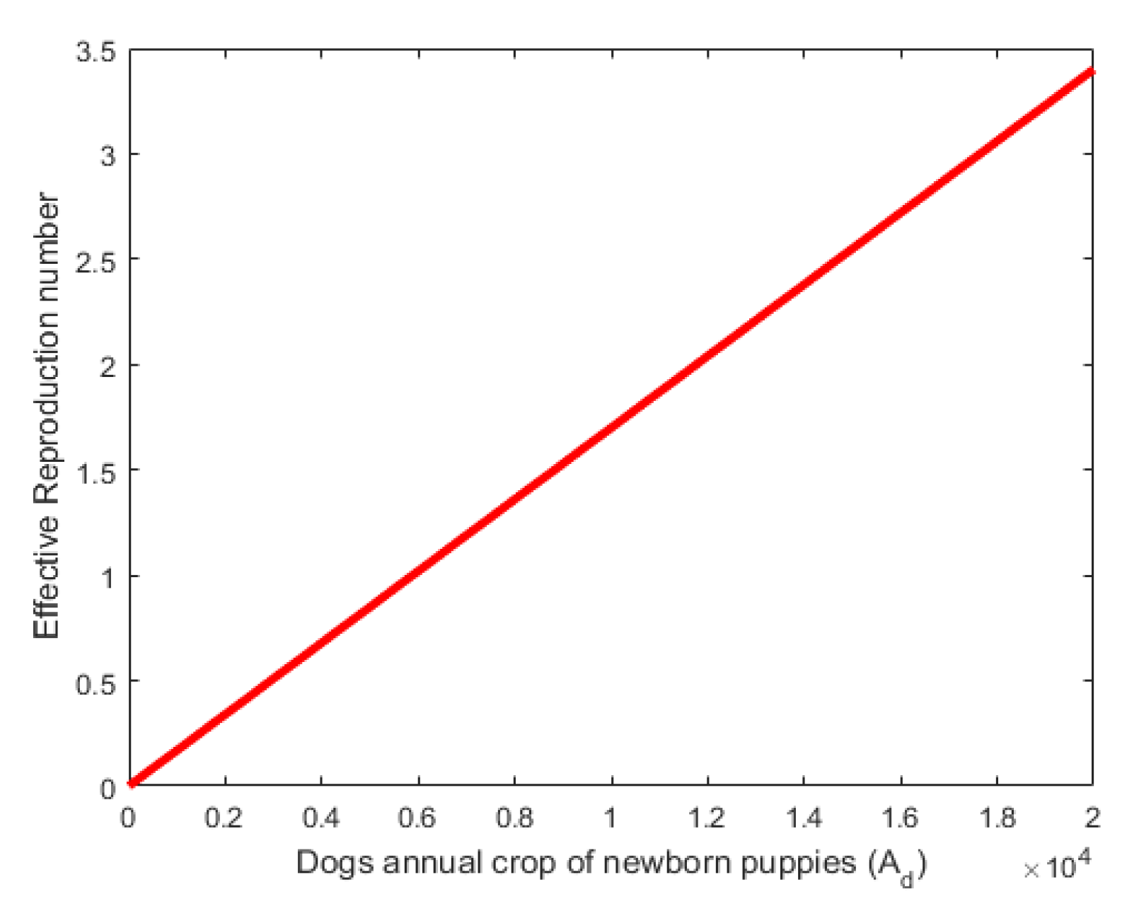
We observe the sensitivity index values’ sign. The parameters ( A d , β d P , β d F ,   δ d , and   α d ) which have positive indices, indicate that they have a significant effect on the spread of the disease within the community. As their values increase, the community’s average number of secondary case infections increases due to an increase in the effective reproduction number ( R e ) i.e., the parameters ( A d , β d P , β d F ,   δ d , and   α d ) directly proportional to R e . In addition, the parameters (   v d , θ d , c d , ρ d , and ε d ) with negative sensitivity indices have an impact on decreasing the disease burden in the community when their values increase while the others remain unchanged. Also, as their values increase, the effective reproduction number ( R e ) decreases, minimizing the disease’s widespread within the community i.e., inversely proportional to R e [13]. The relationship between the parameters ( A d , β d P , β d F ,   δ d ,   θ d ,   δ d , ε d ) and the effective reproductive number is numerically simulated and is displayed in the figures below.
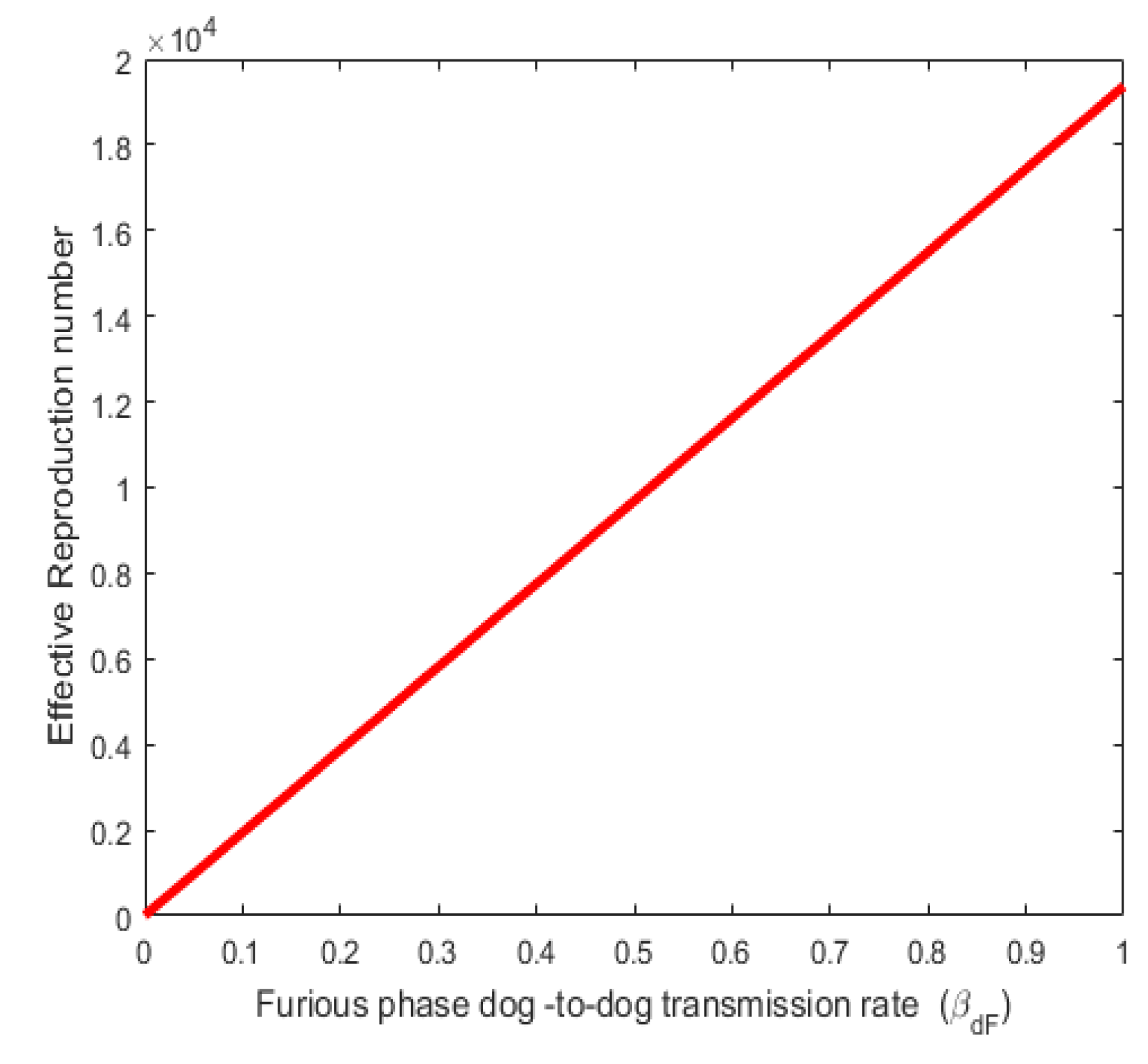
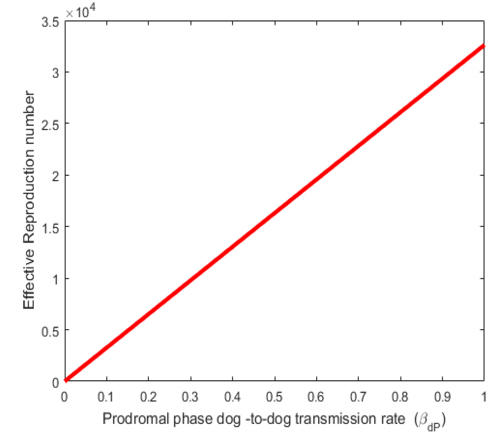
Figure 2. Shows a direct relationship between the effective reproduction number (Re) and Furious phase dog-to-dog transmission rate β d F . Also, Figure 3 shows a direct relationship between the effective reproduction number ( R e ) and the Prodromal phase dog-to-dog transmission rate. Both the infection rates β d F , and β d P values varied as shown in Figure 2 and Figure 3. The result agrees with reality in the sense that as the rate of infection rabies increases, the number of individuals that will be infected in the population also increases thereby increasing the effective reproduction number.
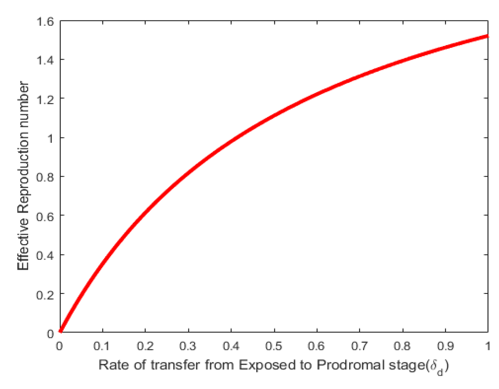
Figure 4. Shows that the effective reproduction numbe (Re) is an increasing function of of the recruitment rate A d . Here the values of the recruitment rate A d   were varied as shown in the figure. This shows that direct relationship between the annual birth rate of the dog population and the effective reproductive number. In Figure 6, the effective reproduction number   R e varies directly with the rate of transfer from Exposed to Prodromal stage   δ d . Values of δ d   were varied as shown in the figure.
Figure 4. Effect of parameter A d on R e
Preprints 102423 g004
Figure 5. Effect of parameter δ d on R e
Preprints 102423 g005
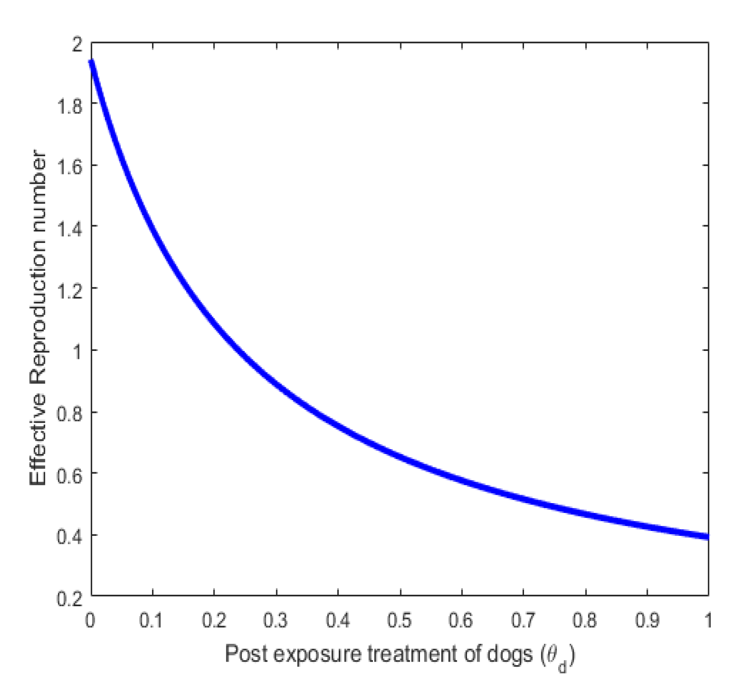
Figure 6. Effect of parameter θ d on R e
Preprints 102423 g006
Figure 6 shows an inverse relationship between the effective reproduction number   R e and the recovery rate θ d due to post-exposed treatment. This is true because if proper treatment is given to Exposed individual dogs, fewer people will be infected thereby reducing the effective reproduction number   R e .
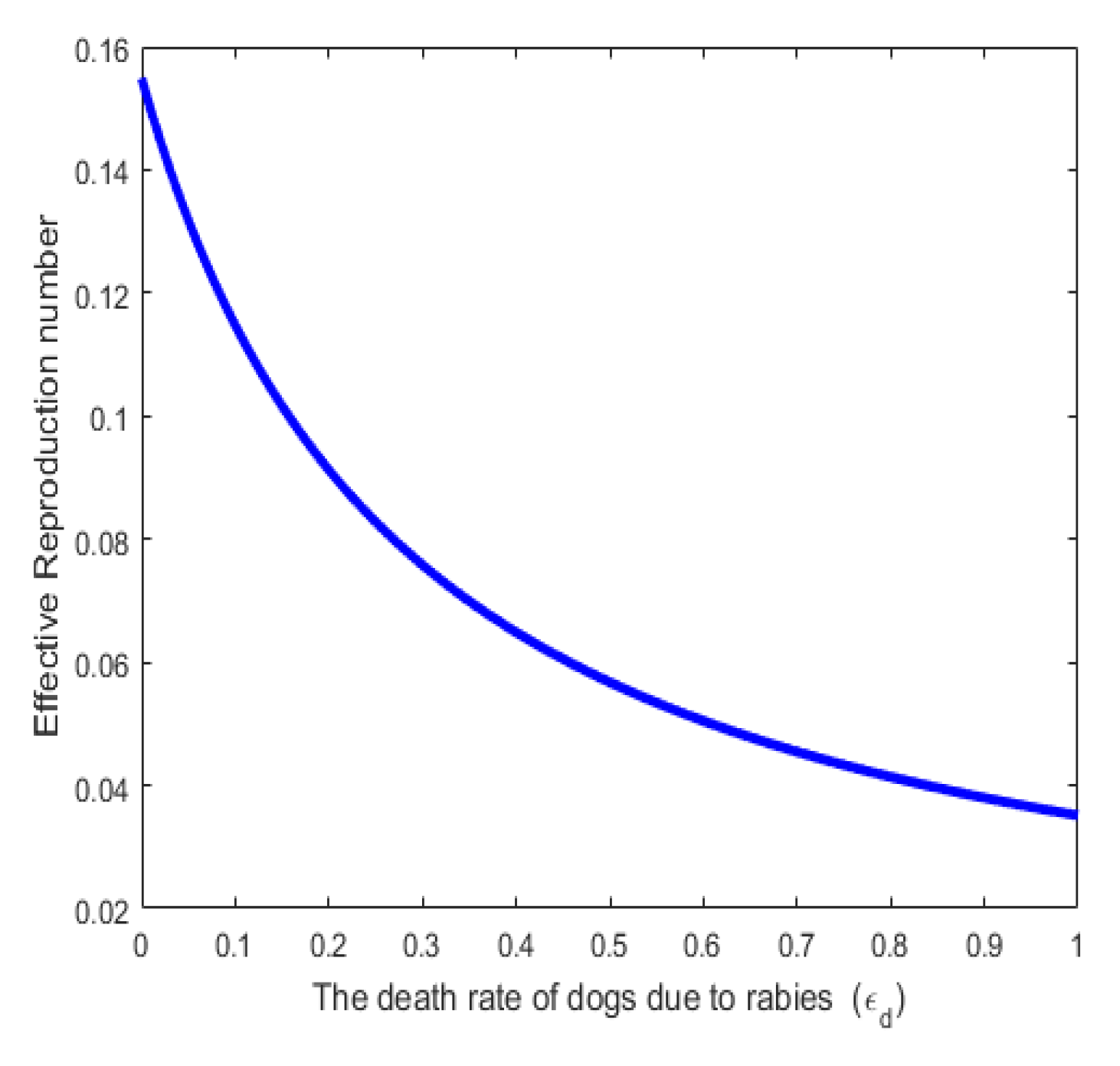
Figure 7. Effect of parameter ε d on R e
Preprints 102423 g007
In Figure 7. The effective reproduction number   R e is a decreasing function of rabies-induced death ε d . Values of ε d   were varied as shown in the figure. This also agrees with reality because as more infectious individuals die as a result of rabies infection, the infection rate will also be reduced.

5. Analysis of the Optimal Control Model

This section does a detailed study of the time-dependent rabies model, given by the system (1). Pontryagin’s Maximum Principle [14], which has been widely used in mathematical models of biological processes including optimal forms the basis of the analysis [15, 16]. The following goal or cost-functional is used to decrease the populations of infectious dogs in the prodromal phase,     I d P , and infectious dogs in the furious phase   I d F , as well as exposed humans E h   and infectious humans   I h . Our goal is to minimize the objective function by identifying the most efficient controls, such as u i t , ( i = 1 ,   2 ,   3 ,   4 ) : .
Our objective function becomes
J = min u U 0 T   A 1 E d + A 2 E h + A 3 I d P + A 4 I d F + A 5 I h + 1 2   i = 1 4 B i   u i 2   ( t ) d t
subject to the model (1),
  d S d d t = A d β d P I d P + β d F I d F S d μ d + u 1 S d   + α d R d   d E d d t = ( β d P I d p + β d F I d F ) S d μ d + δ d + u 2 E d   d I d p d t = δ d E d μ d + ρ d + c d I d P   d I d F d t = ρ d I d P μ d + ε d + c d I d F   d R d d t = u 1 S d + u 2 E d μ d + α d R d     d S h d t = A h ( β h P I d P + β h F I d F ) S h μ h + u 3 S h + α h R h   d E h d t = ( β h P I d P + β h F I d F ) S h μ h + δ h + u 4 E h   d I h d t = δ h E h μ h + ε h I h     d R h d t = u 3 S h + u 4 E h μ h + α h R h  
where A 1 , and A2, are the weight constants of the exposed dog and human class, A 3 ,   and A 4 are the weight constants of prodromal and Furious phase infectious dog classes, and A 5 are the weight constants of the infectious human class. Similarly, B 1 u   1 2 ,   B 2 u   2 2 ,   B 3 u   3 2 ,   and B 4 u   4 2 describe the cost associated with rabies vaccination and treatment. In this work, as in other studies [17, 18], the cost control functions take a quadratic form. We want to find the optimal control u i * = u 1 * , u 2 * ,   u 3 * ,   u 4 *   such as
J u 1 * , u 2 * ,   u 3 * ,   u 4 *   = min J { u 1 ,   u 2 ,   u 3 ,   u 4   |   u i U   for   i = 1 ,   2 ,   3 ,   4 }  
subject to the control set provided by the dynamical system in (1)
U = { u 1 ,   u 2 ,   u 3 ,   u 4 } such that, 0 u i 1 for i = 1 ,   2 ,   3 ,   4 } ; L e b e s g u e m e a s u r a b l e   t 0 ,   T , the non-empty control set.

5.1. Characterization of the Optimal Control

The Pontryagin’s Maximum Principle [14] is used to try and obtain the necessary conditions for the optimal control of rabies governed by the non-autonomous system. This principle becomes the state system (1), with the objective functional (4.1) and (4.2), into a pointwise minimizing problem concerning the controls u 1 ,   u 2 ,   u 3   a n d   u 4 .
The Hamiltonian equation with state variables S d = S d * , E d = E d * ,   I d P = I d P * , I d F = I d F * , R d = R d * , S h = S h * , E h = E h * ,   I h = I h * , and R h = R h * is formed as
H = I i n t e g r a n d + ( a d j o i n s ) × ( R H S ) of the
  H = A 1 E d * + A 2 E h * + A 3 I d P * + A 4 I d F * + A 5 I h *   + 1 2   B 1 u   1 2 + B 2 u   2 2 + B 3 u   3 2 + B 4 u   4 2   + λ 1 A d β d P I d P * + β d F I d F * S d * μ d + u 1 S d *   + α d R d *   4.3   + λ 2 β d P I d P * + β d F I d F * S d * μ d + δ d + u 2 E d *   + λ 3 δ d E d * μ d + ρ d + c d I d P *     + λ 4 ρ d I d P * μ d + ε d + c d I d F *     + λ 5 u 1 S d * + u 2 E d * μ d + α d R d *     + λ 6 [ A h β h P I d P * + β h F I d F * S h * ( μ h + u 3 ) S h * + α h R h *   ]   + λ 7 β h P I d P * + β h F I d F * S h * μ h + δ h + u 4 E h *     + λ 8   δ h E h * μ h + ε h I h *   + λ 9 u 3 S h * + u 4 E h * μ h + α h R h *    
where the adjoint (co-state) variables are λ i , i = 1, 2, 3, 5, 6, 7, 8, 9. The necessary conditions for the optimal control by the following result.
Theorem4.2:Given an optimal control quadruple u 1 * , u 2 * , u 3 * , u 4 * that minimizes objective functional (4.1) over the control set U subject to the state system (1), then there exist adjoint variables λ 1 , λ 2 , λ 3 , λ 4 , λ 5 , λ 6 , λ 7 , λ 8 , λ 9 satisfying
d λ 1 d t = λ 1 β d P I d P * + β d F I d F * + μ d + u 1 λ 2 β d P I d P * + β d F I d F * λ 5 u 1
d λ 2 d t = λ 2 μ d + δ d + u 2 λ 3 δ d λ 5 u 2 A 1
d λ 3 d t = λ 1 β d P S d * + λ 3 μ d + ρ d + c d + λ 6 β h P S h * λ 2 β d P S d *
λ 4 ρ d λ 7 β h P S h * A 3   4.4
d λ 4 d t = λ 1 β d F S d * + λ 4 μ d + ε d + c d + λ 6 β h F S h * λ 2 β d F S d * λ 7 β h F S h * A 4  
  d λ 5 d t = λ 5 μ d + α d λ 1 α d
d λ 6 d t = λ 6 β h P I d P * + β h F I d F * + λ 6 μ h + u 3 λ 7 β h P I d P * + β h F I d F * λ 9 u 3
d λ 7 d t = λ 7 μ h + δ h + u 4 λ 8 δ h λ 9 u 4 A 2
d λ 8 d t = λ 8 μ h + ε h A 5
d λ 9 d t = H R h * = λ 6 α h + λ 9 μ h + α h
With transversely conditions, λ i T = 0 , i = 1 ,   2 ,   3 ,   4 ,   5 ,   6 ,   7 ,   8 , 9 i.e.,
λ 1 T = 0 ,   λ 2 T = 0 ,   λ 3 T = 0 ,     λ 4 T = 0 ,   λ 5 T = 0 ,   λ 6 T = 0 ,
λ 7 T = 0 ,   λ 8 T = 0 ,   λ 9 T = 0 , 4.5
And
u 1 * = m i n   m a x 0 ,   ( λ 1 λ 5 ) S d * B 1 ,   1
u 2 * = m i n   m a x 0 ,   ( λ 2 λ 5 ) E d * B 2 ,   1
u 3 * = m i n   m a x 0 ,   ( λ 6 λ 9 ) S h * B 3 ,   1
u 4 * = m i n   m a x 0 ,   ( λ 7 λ 9 ) E h * B 4 ,   1
Proof: 
By considering partial derivatives of the Hamiltonian H given by (4.3) with respect to the corresponding state variables, one can get the adjoint equations governed by the non-autonomous system (4.4).
d λ 1 d t = H S d * ,   d λ 2 d t = H E d * ,   d λ 3 d t = H I d P * ,   d λ 4 d t = H I d F * ,   d λ 5 d t = H R d *
d λ 6 d t = H S h * ,   d λ 7 d t = H E h *   ,   d λ 8 d t = H I h *   , d λ 9 d t = H R h *
d λ 1 d t = H S d * = λ 1 β d P I d P * + β d F I d F * + μ d + u 1 λ 2 β d P I d P * + β d F I d F * λ 5 u 1
d λ 2 d t = H E d * = λ 2 μ d + δ d + u 2 λ 3 δ d λ 5 u 2 A 1
d λ 3 d t = H I d P * = λ 1 β d P S d * + λ 3 μ d + ρ d + c d + λ 6 β h P S h * λ 2 β d P S d *
λ 4 ρ d λ 7 β h P S h * A 3
d λ 4 d t = H I d F * = λ 1 β d F S d * + λ 4 μ d + ε d + c d + λ 6 β h F S h * λ 2 β d F S d * λ 7 β h F S h * A 4
d λ 5 d t = H R d * = λ 5 μ d + α d λ 1 α d
d λ 6 d t = H S h * = λ 6 β h P I d P * + β h F I d F * + λ 6 μ h + u 3 λ 7 β h P I d P * + β h F I d F * λ 9 u 3
d λ 7 d t = H E h * = λ 7 μ h + δ h + u 4 λ 8 δ h λ 9 u 4 A 2
d λ 8 d t = H I h * = λ 8 μ h + ε h A 5
d λ 9 d t = H R h * = λ 6 α h + λ 9 μ h + α h
Under terminal conditions or transversality (4.5). Additionally, the following partial differential equations must be solved to determine the optimal control characterization given by (4.6):
H u i = 0 ,   i = 1 ,   2 ,   3 ,   4 .   The optimality condition gives us
H u 1 | u 1 = u 1 * = B 1 u 1 * λ 1 S d * + λ 5 S d * = 0   i . e . ,   u 1 * = λ 1 λ 5 S d * B 1
H u 2 | u 2 = u 2 * = B 2 u 2 * λ 2 E d * + λ 5 E d * = 0   i . e . ,   u 2 * = ( λ 2 λ 5 ) E d * B 2
H u 3 | u 3 = u 3 * = B 3 u 3 * λ 6 S h * + λ 9 S h * = 0   i . e . ,   u 3 * = ( λ 6 λ 9 ) S h * B 3
H u 4 | u 4 = u 4 * = B 4 u 4 * λ 7 E h * + λ 9 E h * = 0   i . e . ,   u 4 * = ( λ 7 λ 9 ) E h * B 4
By standard control arguments involving bounds on the control, then
u i * =   0 ,   i f   φ i *   0   φ i *   i f   0 φ i *   1 1   i f   φ i *   1  
for i = 1 ,   2 ,   3 ,   4 and where
φ 1 * = λ 1 λ 5 S d * B 1
φ 2 * = ( λ 2 λ 5 ) E d * B 2
φ 3 * = ( λ 6 λ 9 ) S h * B 3
φ 4 * = ( λ 7 λ 9 ) E h * B 4
The proof is now complete.

6. Simulations and Cost-Effectiveness Analysis

The numerical simulations of the optimality system and the cost-effectiveness analysis of some of the control strategy combinations under consideration are the primary focus of this part.

6.1. Numerical Simulations

The state system (1) together with the adjoint equations (4.4) containing the initial conditions at t = 0, the terminal conditions (4.5), and the optimal control’s characterization (4.6) form the optimality system. Using an iterative approach and a fourth-order forward-backward Runge-Kutta scheme, this optimality system is solved. with the initial conditions at t = 0 for the controls throughout the simulated time, the state system (1) is solved forward in time. Because of the terminal conditions (4.5), the adjoint system is solved backward in time using the state equations’ current iteration responses. The specifics of the numerical process for solving this kind of optimality system with various time orientations are provided [19]. The parameter values from Table 2 are used to show how different combinations of the optimal control intervention options influence the population’s risk of developing rabies. with initial conditions : S d = 1000000 , E d = 8000 ,   I d P = 150 ,   I d F = 250 , R d = 50000 ,   S h = 5,000,000   E h = 100 ,   I h = 38 , and R h = 2500 , . The weight constants values are chosen as A 1 = A 2 =   A 3 =   A 4 = A 5 = B 1 = B 3 = 1 and B 2 = B 4 = 4

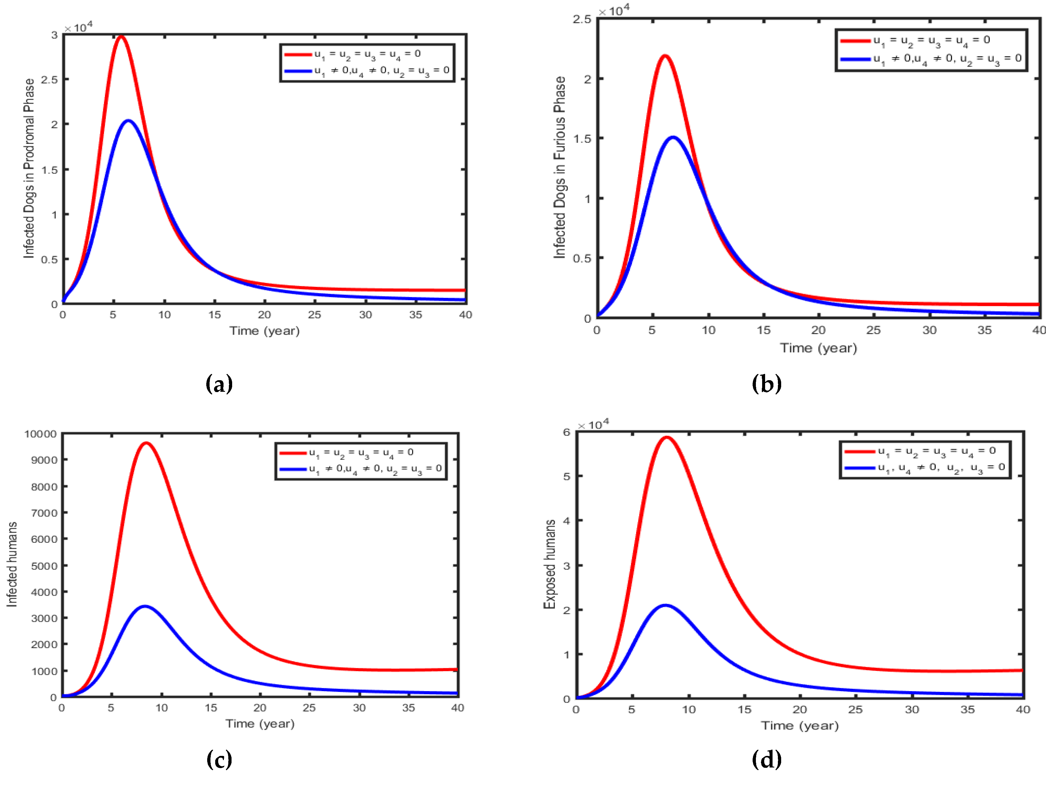
6.1.1. Intervention 1: Optimal Use of Pre-Exposed Prophylaxis and Treating the Exposed Dogs
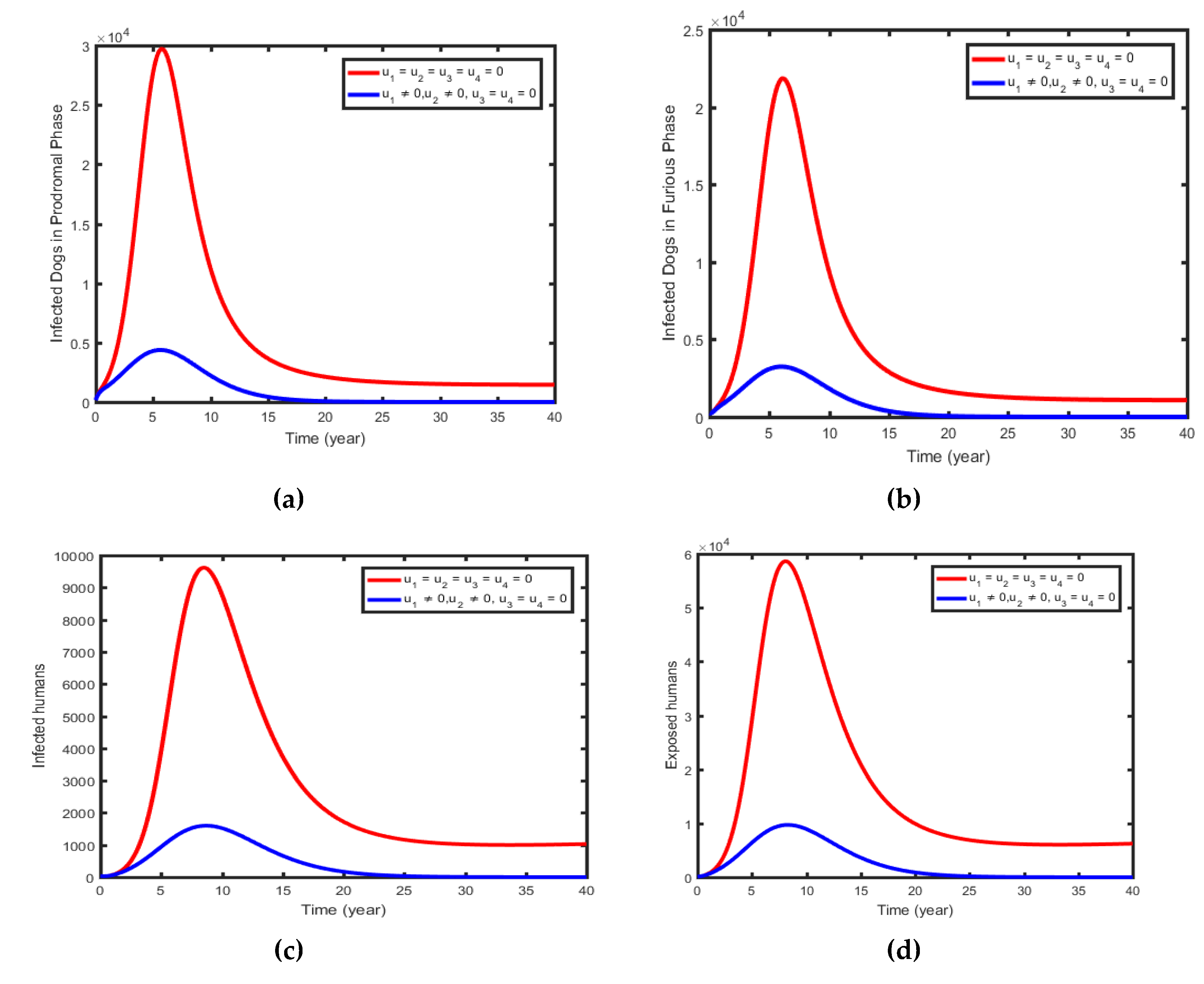
This intervention method combines the control effort to treat the exposed dogs, with the control effort to increase immunity in susceptible dogs (i.e., u 1 ,   u 2 0 ) . The magnitudes of infected prodromal phase dogs, infected furious phase dogs, and infectious, and exposed humans decrease more rapidly when controls are in use than in the case without controls, as Figure 6(a-d) shows.
Figure 6. Simulations of the Optimal Control showing the effect of control Strategy 1.
Preprints 102423 g008

6.1.2. Intervention 2: Optimal Use of Pre-Exposed Prophylaxis Dogs and Pre-Exposed Prophylaxis Humans
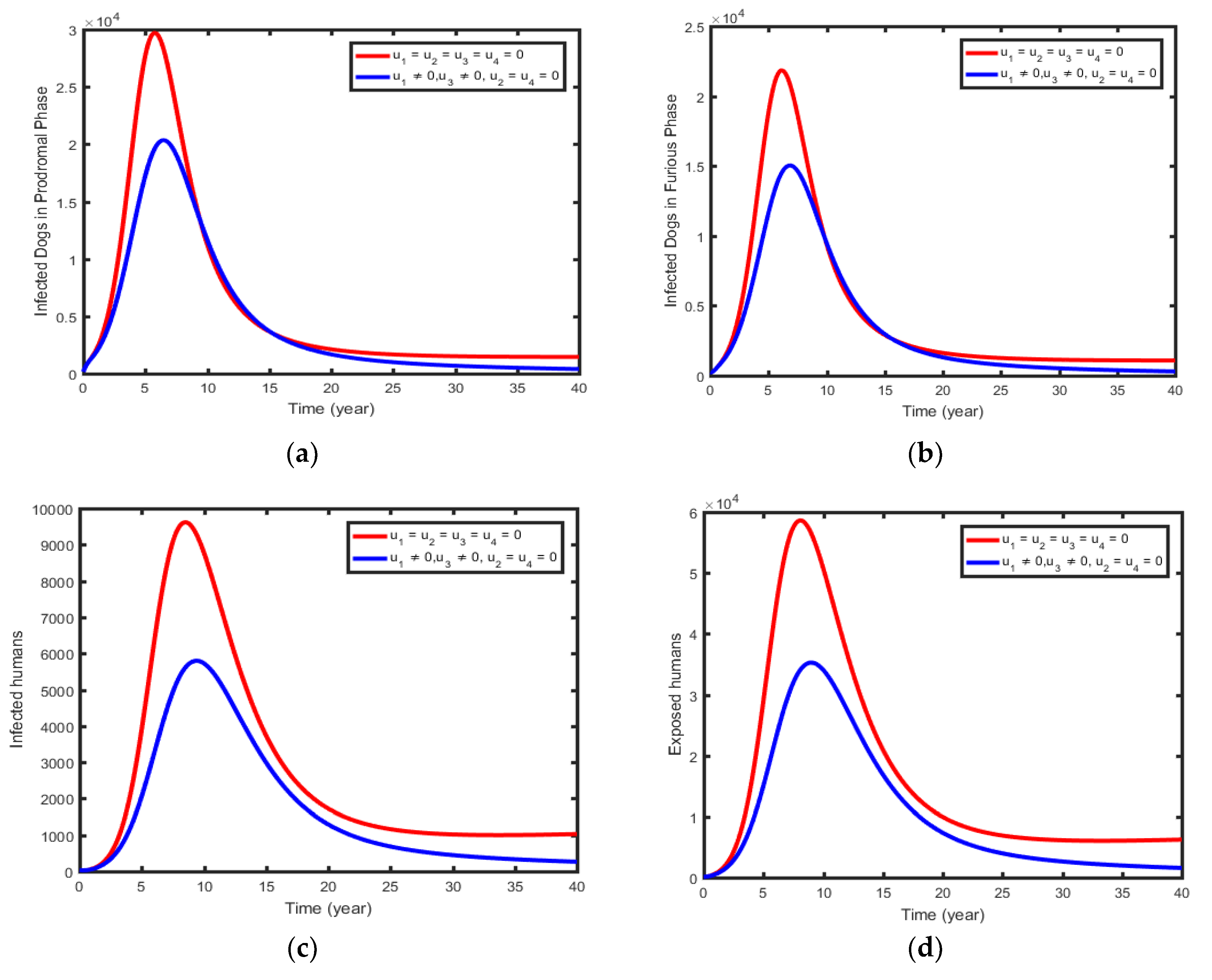
Figure 7 shows this intervention method, which combines the optimal use of control effort to increase susceptible dog’s immunity and control effort to increase susceptible human immunity (i.e., u 1 u 3 0 ) . The magnitudes of infected prodromal phase dogs, infectious furious phase dogs, and infectious, and exposed humans decrease more quickly in the presence of controls than in the absence of controls, as Figure 7(a-d) shows.
Figure 7. Simulations of the Optimal Control showing the effect of control Strategy 2.
Preprints 102423 g009

6.1.3. Intervention 3: Optimal Use of Dogs Per-Exposed Prophylaxis and Human Post-Exposed Prophylaxis

This strategy illustrates combines the optimal use of the control effort to increase the immunity of susceptible dogs (per-exposed prophylaxis for dogs) and the control effort at treating the exposed humans (post-exposed prophylaxis for humans) i.e., u 1 ,   u 4 0 . As expected, the numbers of infectious prodromal phase dogs (Figure 8a), infectious furious phase dogs (Figure 8b), and infectious and Exposed humans (Figure 8c & 8d) diminish more rapidly with controls than the case without controls.

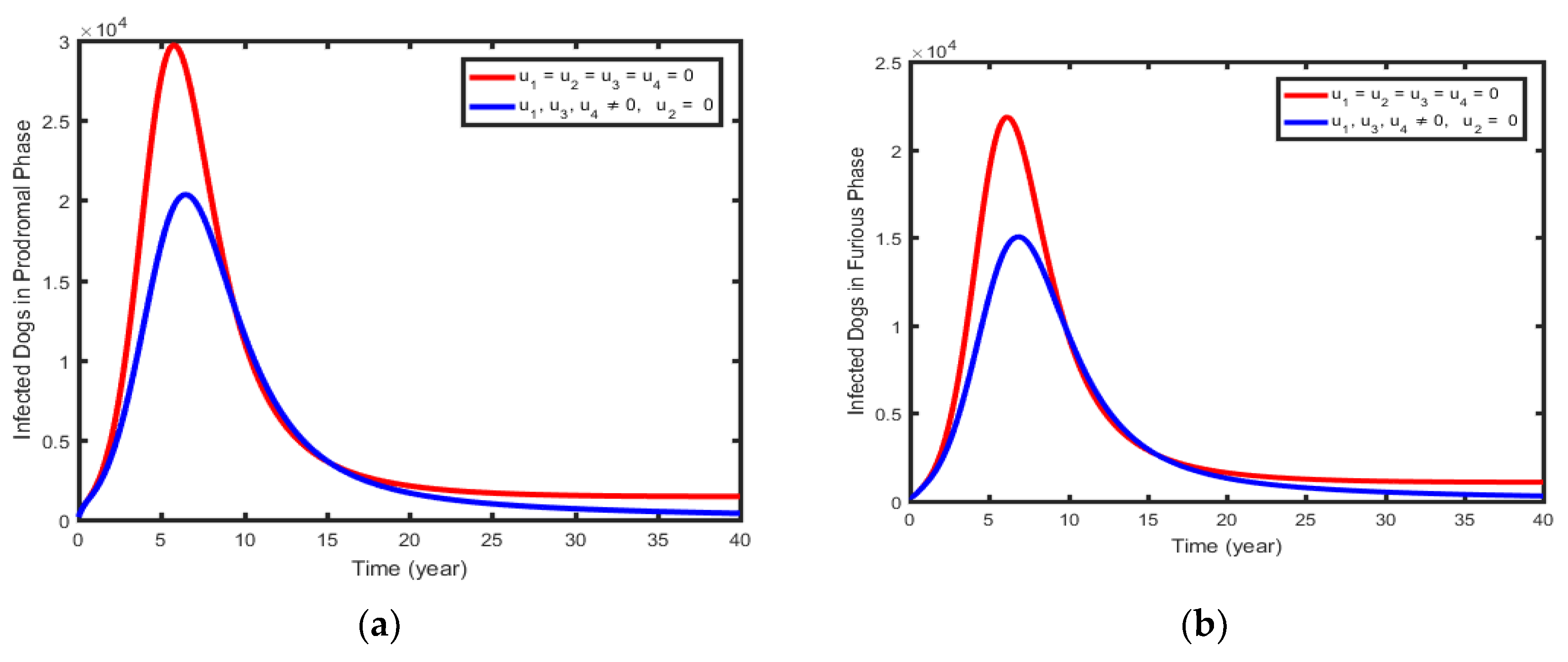
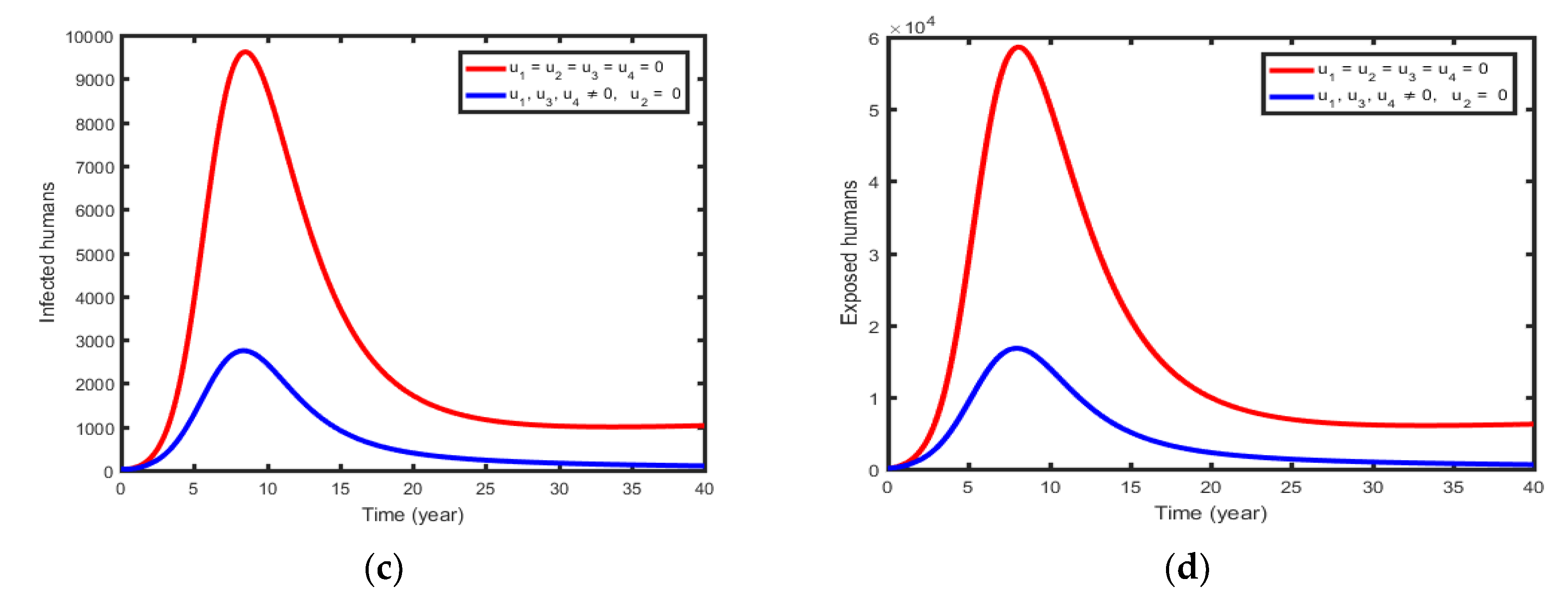
6.1.4. Intervention 4: Optimal Use of Dogs Per-Exposed Prophylaxis, Human’s Per-Exposed Prophylaxis and Human’s Post-Exposed Prophylaxis

This strategy shows the control effort to increase the immunity of susceptible dogs, the control effort increasing the immunity of susceptible humans, and the control effort treating the exposed humans ( u 1 ,   u 3 ,   u 4 0 ) . on the spread of rabies dynamics in the population. Figure 9(a) and 9(b) display that the controls decrease the size of infectious in prodromal and Furious phase dogs more rapidly than when controls are not applied. Similarly, the numbers of infectious humans (Figure 9c) and infectious-exposed humans (Figure 9d) decreased more rapidly with controls than the case without controls.

6.1.5. Intervention 4: Implementing All Optimal Control Strategies

This uses the four controls ( u 1 t ,     u 2 t ,   u 3 t ,   and u 4 t to minimize the spread of rabies governed by the model (1). The sizes of infectious in prodromal (Figure 9a), Furious phase dogs (Figure 9b), infectious humans (Figure 9c), and exposed humans (Figure 9d), rapidly decrease when controls are in use than the case when controls are not used intervention strategy.

7. Cost-Effectiveness Analysis

We can determine the most effective and least expensive method based on the optimality system’s simulation result using the parameter values listed in Table 2. We used a technique known as the incremental cost-effectiveness ratio (ICER) to arrive at this strategy.
I C E R = C h a n g e   i n   t o t a l   c o s t   c h a n g e   i n   c o n t r o l   b e n e f i t s
By using this method, we were able to compare exceed techniques with more than unity and evaluate which intervention was more effective than the next less effective one. The ratio of the difference in the total number of infections averted to the difference in the averted costs between the two methods was the definition of this technique [19]. We computed the overall cost saved and the total number of infections saved based on the simulation result of the optimal control problem. Based on the total number of infections averted, the control measures are arranged in increasing order in Table 4. The total number of infections prevented was calculated as the difference between the total number of people infected with rabies with controls and the total number of people infected with rabies without controls. The cost function represented by 1 2 B 1 u   1 2 ,   1 2 B 2 u   2 2 ,   1 2 B 3 u   3 2 ,   a n d   1 2 B 4 u   4 2   over was used to determine the total number of infections prevented [19]. Table 3 shows the overall number of diseases prevented and the total cost of all interventions. However, as a single control is unsuccessful in completely eradicating the rabies virus from the human population, we did not take into consideration a strategy that applies only one single control.
we implement the following combinations of the controls.
Strategy 1: The control effort to increase the immunity of susceptible dogs and the control effort aimed at treating the exposed dogs (i.e., u 1 u 2 0 ) .
Strategy 2: The control effort to increase the immunity of susceptible dogs and the control effort aimed at increasing the immunity of susceptible humans (i.e., u 1 u 3 0 ) .
Strategy 3: The control effort to increase the immunity of susceptible dogs and the control effort aimed at treating the exposed humans (i.e., u 1 u 4 0 ) .
Strategy 4: The control effort to increase the immunity of susceptible dogs, the control effort aimed at increasing the immunity of susceptible humans and the control effort aimed at treating the exposed humans (i.e., u 1 u 3 u 4 0 ) .
Strategy 5: Implementing all controls (i.e., u 1 u 2 u 3 u 4 0 )
I C E R 2 = 44,140,000 1,046,800 = 42.16660   ,   I C E R 3 = 5876000 832380 = 7.05928
I C E R   ( 2 ) > I C E R   ( 3 ) , as can be shown. This indicates that strategy 2 is less successful and more expensive than approach 3. As a result, strategy 2 is removed from the list of alternative interventions, and strategies 3 and 4’s ICER are recalculated, as seen in Table 7.
I C E R 3 = 38,264,000 1,879,180 = 20.36207 ,   I C E R 4 = 1229000 174060 = 7.06078
Given that ICER(3) > ICER(4), approach 3 is dominant over strategy 4, more expensive, and less successful. As a result, strategy 3 is removed from the list of alternative interventions, and strategies 4 and 1’s ICER are revised as shown in Table 8.
I C E R 4 = 37,035,000 2,053,240 = 18.03734 ,   I C E R 1 = 28385900 295140 = 96.17775
I C E R ( 4 ) > I C E R ( 1 ) , as could have been observed. This indicates that compared to approach 1, strategy 4 is less effective and more expensive. As a result, strategy 4 is removed from the list of alternative interventions, and strategies 1 and 5’s ICER are recalculated, as shown in Table 9.
I C E R 1 = 8,649,100 2,348,380 = 3.68301 , I C E R 5 = 1,977,900 280,490 = 7.06078 Table 9 shows that ICER (1) is greater than ICER (5). This suggests that compared to strategy 5, approach 1 is less effective and more expensive. Thus, out of all the techniques examined in this study, intervention strategy 5 is thought to be the most cost-effective (the most economical).

8. Conclusion and Recommendations

8.1. Conclusion

The dynamics of rabies infection in a human population and among dogs are being studied using a nonlinear mathematical model that is proposed in this study. Because the behaviors of the prodromal and furious phases of infection differ, the model assumes that the infected dog’s compartment was divided into two. Based on these different behaviors, the transmission rate of dogs was divided into two for each population, i.e., β d P ,   β d F ,   β h P , and β h F . Additionally, to simulate the effect of those parameters, we solved the model for different values of the most significant model parameters. Figure 4, Figure 5, Figure 6, Figure 7 and Figure 8 show the results. The parameters A d , β d P , β d F ,   δ d ,   α d , and   α d have a positive relationship with the effective reproduction number ( R e ) based on a sensitivity analysis of the parameter. On the other hand, the parameters μ d ,   v d , θ d ,   c d , ρ d , and ε d are negative signs, then these are inversely proportional to the effective number ( R e ) . By adding time-dependent controls to the base model, the model is expanded to an optimum control problem, and the optimality conditions are obtained by applying Pontryagin’s Maximum Principle. Lastly, to determine the effectiveness of different control combinations, numerical simulations of the resulting control problem are performed. The simulation of the control problem shows that the most effective strategy for controlling the disease is the one that makes use of all relevant control measures. Therefore, preventing the spread of rabies requires a multipronged strategy.

8.2. Recommendations

From the results of this study, we suggest the following points to control/minimize/ Dog rabies disease:
  • ✓ The dynamics of rabies transmission should be investigated more thoroughly to develop the optimal control measures.
  • ✓ Workshops, seminars, and trainings are examples of educational initiatives that should be conducted to raise awareness regarding rabies transmission and prevention strategies.
  • ✓ Dog owners should be encouraged by media coverage to crate their pets rather than allow them free reign on the streets.
  • ✓ The government and policymakers should come up with strategies to control and reduce the number of stray dogs. A plan that confines owned dogs to specific locations to restrict the annual crop of newborn puppies and lower the frequency of dog-to-dog transmission.
  • ✓ The primary focus of strategy development should be on implementing the most effective control methods, such as vaccinating dog populations, decreasing the annual number of newborn puppies, and removing stray dogs, to reduce the human population and rapidly eliminate diseases.

Data Availability Statement

The data used to support the findings of this manuscript are available from the corresponding author upon request.

Conflicts of Interest

The authors declare that they have no known competing financial interests or personal relationships that could have appeared to influence the work reported in this paper.

References

  1. Asfaw, G. B., Abagero, A., Addissie, A., Yalew, A. W., Watere, S. H., Desta, G. B., ... & Deressa, S. G. (2024). Epidemiology of suspected rabies cases in Ethiopia: 2018–2022. One Health Advances, 2(1), 3. [CrossRef]
  2. Shigui Ruan, (2017). Modeling the transmission dynamics and control of rabies in China. Mathematical. Biosciences Volume 286, April, Pages 65-93.
  3. Musaili, J. S., & Chepkwony, I. (2020). A Mathematical Model of Rabies Transmission Dynamics in Dogs Incorporating Public Health Education as a Control Strategy-A Case Study of Makueni County. Journal of Advances in Mathematics and Computer Science, 35(1), 1-11. [CrossRef]
  4. Eze, O. C., Mbah, G. E., Nnaji, D. U., & Onyiaji, N. E. (2020). Mathematical modelling of transmission dynamics of rabies virus. International Journal of Mathematics Trends and Technology-IJMTT, 66.
  5. Thongtha, A., & Modnak, C. (2021). A mathematical modeling of rabies with vaccination and culling. International Journal of Biomathematics, 14(06), 2150039. [CrossRef]
  6. Pantha, B., Giri, S., Joshi, H. R., & Vaidya, N. K. (2021). Modeling transmission dynamics of rabies in Nepal. Infectious Disease Modelling, 6, 284-301. [CrossRef]
  7. Iggidr, A., Mbang, J., Sallet, G., & Tewa, J. J. (2007, August). Multi-compartment models. In Conference Publications (Vol. 2007, No. Special, pp. 506-519). Conference Publications.
  8. Edward, S., & Nyerere, N. (2015). A mathematical model for the dynamics of cholera with control measures. Applied and computational Mathematics, 4(2), 53-63. [CrossRef]
  9. Josephine, E. A. (2009). The basic reproduction number: Bifurcation and stability. A PGD thesis submitted to the African Institute of Mathematical Sciences.
  10. Hailemichael, D. D., Edessa, G. K., & Koya, P. R. (2023). Mathematical Modeling of Dog Rabies Transmission Dynamics Using Optimal Control Analysis. Contemporary Mathematics, 296-319.
  11. Asamoah, J. K. K., Oduro, F. T., Bonyah, E., & Seidu, B. (2017). Modelling of rabies transmission dynamics using optimal control analysis. Journal of Applied Mathematics, 2017.
  12. Ega, T. T., Luboobi, L., & Kuznetsov, D. (2015). Modeling the dynamics of rabies transmission with vaccination and stability analysis.
  13. Hailemichael, D. D., Edessa, G. K., & Koya, P. R. (2022). Effect of vaccination and culling on the dynamics of rabies transmission from stray dogs to domestic dogs. Journal of Applied Mathematics, 2022. [CrossRef]
  14. Pontryagin, L.S. (2018). Mathematical theory of optimal processes. Routledge.
  15. Olaniyi, S. , Okosun, K. O., Adesanya, S. O., & Lebelo, R. S. (2020). Modelling malaria dynamics with partial immunity and protected travellers: optimal control and cost-effectiveness analysis. Journal of biological dynamics, 14(1), 90-115. [CrossRef]
  16. Olaniyi, S.J.A.M. (2018). Dynamics of Zika virus model with nonlinear incidence and optimal control strategies. Appl. Math. Inf. Sci, 12(5), 969-982. [CrossRef]
  17. Modnak, C. (2017). Mathematical modelling of an avian influenza: optimal control study for intervention strategies. Appl. Math. Inf. Sci, 11(4), 1049-1057. [CrossRef]
  18. Hugo, A., Makinde, O. D., Kumar, S., & Chibwana, F. F. (2017). Optimal control and cost effectiveness analysis for Newcastle disease eco-epidemiological model in Tanzania. Journal of Biological Dynamics, 11(1), 190-209. [CrossRef]
  19. Lenhart, S., & Workman, J. T. (2007). Optimal control applied to biological models. Chapman and Hall/CRC.
  20. Renalda, E. K., Kuznetsov, D., & Kreppel, K. (2020). Desirable Dog-Rabies Control Methods in an Urban setting in Africa-a Mathematical Model.
  21. Sharma, P. M., Dobhal, Y., Sharma, V., Kumar, S., & Gupta, S. (2015). Rabies: Understanding Neuropathology and Management. Int. J. Heal. Sci. Res, 5, 320-332.
Figure 1. Model Diagram.
Preprints 102423 g001
Figure 2. Effect of parameter β d F on R e .
Preprints 102423 g002
Figure 3. Effect of parameter β d P   on R e .
Preprints 102423 g003
Figure 8. Simulations of the Optimal Control showing the effect of control Strategy 3.
Preprints 102423 g010
Figure 9. Simulations of the Optimal Control showing the effect of control Strategy 4.
Preprints 102423 g011aPreprints 102423 g011b
Figure 10. Simulations of the Optimal Control showing the effect of control Strategy 5.
Preprints 102423 g012
Table 2. Parameters and their values for model (1) (unit: year-1).
Parameter Value Interpretation Source
A d 15900 Dogs annual crop of newborn puppies Assumed
β d P 1.28 × 10 8 Prodromal dog-to-dog transmission rate Assumed
β d F 1.10 × 10 5 Furious dog-to-dog transmission rate Assumed
δ d 0.17 The incubation period of dog populations [12]
ρ d 0.821 Rate of prodromal to furious stage Assumed
v d 0.25 Pre-exposure prophylaxis for dogs [11]
θ d 0.2 Post-exposure prophylaxis for dogs [11]
ε d 1 The death rate of dogs due to rabies [11]
μ d 0.056 The natural death rate of dogs [11]
c d 0.01792 Rabid dog culling rate [20]
α d 1 Loss of immunity in dogs [11]
A h 112980 Human annual birth [12]
β h P 9.79 × 10 10 Prodromal dog-to-human transmission rate Assumed
β h F 9.86 × 10 8 Furious dog-to-human transmission rate Assumed
δ h 0.1667 The incubation period of human populations [12]
v h 0.2 Pre-exposure prophylaxis for humans Assumed
θ h 0.2 Post-exposure prophylaxis for humans [11]
ε h 1 The death rate of humans due to rabies [11]
μ h 0.0074 Natural death rate of humans [11]
Table 3. Total number of infections saved and cost averted for all strategies.
Strategy Total infection Averted Total cost ($)
1 2,348,380 8,649,100
2 1,046,800 44,140,000
3 1,879,180 38,264,000
4 2,053,240 37,035,000
5 2,628,870 6,671,200
Table 6. Increasing order of infections averted.
Intervention Total infection Total cost
Strategy Averted ($) ICER
2 1,046,800 44,140,000 42.16660
3 1,879,180 38,264,000 -7.05928
4 2,053,240 37,035,000 -
1 2,348,380 8,649,100 -
5 2,628,870 6,671,200 -
Table 7. Comparison between intervention strategies 3 and 4.
Intervention Total infection Total cost
Strategy Averted ($) ICER
3 1,879,180 38,264,000 20.36207
4 2,053,240 37,035,000 -7.06078
1 2,348,380 8,649,100 -
5 2,628,870 6,671,200 -
Table 8. Comparison between interventions strategy 4 and 1.
Intervention Total infection Total cost
Strategy Averted ($) ICER
4 2,053,240 37,035,000 18.03734
1 2,348,380 8,649,100 -96.17775
5 2,628,870 6,671,200 -
Table 9. Comparison between interventions strategy 1 and 5.
Intervention Total infection Total cost
Strategy Averted ($) ICER
1 2,348,380 8,649,100 3.68301
5 2,628,870 6,671,200 -7.051588
Disclaimer/Publisher’s Note: The statements, opinions and data contained in all publications are solely those of the individual author(s) and contributor(s) and not of MDPI and/or the editor(s). MDPI and/or the editor(s) disclaim responsibility for any injury to people or property resulting from any ideas, methods, instructions or products referred to in the content.
Copyright: This open access article is published under a Creative Commons CC BY 4.0 license, which permit the free download, distribution, and reuse, provided that the author and preprint are cited in any reuse.
Prerpints.org logo

Preprints.org is a free preprint server supported by MDPI in Basel, Switzerland.

Subscribe

© 2024 MDPI (Basel, Switzerland) unless otherwise stated