1. Introduction
Depth estimation, a critical AI technique for predicting depth information, supports various applications. For instance, autonomous driving [
1], drone control [
2], and AR/VR [
3] technologies utilize depth information in various aspects. Among these methodologies, the use of camera devices for depth estimation brings significant advantages, especially in capturing visual information, compared to other methods like LiDARs or infrared sensors. Owing to the visualization capabilities of camera devices, estimation with devices, such as monocular [
4] and stereo cameras [
1], can yield more meaningful information. Especially in object detection [
5], segmentation [
6], and human pose detection [
7], depth prediction with cameras has been utilized proactively. While this essential technology is widely employed in diverse areas, the algorithms always have a trade-off between accuracy and inference time. Accurate AI models tend to be complicated systems, leading to slow estimation. Yet, some applications require fast prediction more than highly accurate depth maps.
Since there is a great demand for rapid-response AI systems, various networks have been proposed to date. MobileNet [
8], which operates with fewer parameters, was developed by Howard et al. and applied to practical cases. Such AI models are sufficiently compact to deploy on mobile phones with high speed but without consuming large power. However, training a compact AI model from scratch often results in a significant decrease in accuracy compared to more complex models. To address this issue, the knowledge distillation method has been proposed, wherein a compact network is trained using the guidance of a more complex model. For instance, Wang et al. [
9] constructed a real-time monocular depth estimation model using knowledge distillation.
However, monocular depth prediction techniques only use RGB images, so optimized training datasets that include similar scenes or features are required for accurate prediction. In contrast, light field depth estimation, which utilizes a light field camera, first developed by Ng et al. [
10], can avoid this problem. Due to this device’s ability to additionally record parallax information, it can inherently capture depth information, unlike monocular cameras. As an example, EPINET proposed by Shin et al. [
11] predicts depth maps with multi-view images as its input. Owing to the complexity of handling multi-view images, the architecture of EPINET is not simple enough to enable real-time inference. In this case, the trade-off between speed and accuracy became an issue too. To tackle this, Hassan et al. [
12] developed a fast convolution algorithm with depth-wise convolution blocks for EPINET. They accelerated the model by a factor of three approximately and slightly increased its prediction accuracy. The method improved the efficiency of convolution calculations. This approach, however, could not prevent a decrease in accuracy when the model’s architecture itself is changed. CNN (Convolutional Neural Network) models generally have the problem of including an excessive number of hyperparameters, such as the number of convolution blocks, filters, and the kernel size suggested by Richter et al. [
13]. This is why our proposed method focuses on simplifying the model’s architecture, which is essential for constructing a compact model.
Therefore, we established a method to create a more compact depth estimation model focusing on EPINET. Our proposed methodology encompasses two primary objectives: one is the reduction of the model’s size to enhance computational efficiency, and the second is the refinement of its accuracy in depth estimation tasks. Initial ablation studies allowed us to explore the balance between accuracy and speed across various EPINET hyperparameters. Through these studies, we identified key modifications in the number of input streams and convolution blocks, significantly contributing to the development of a simplified yet effective model. Furthermore, an internal examination of the convolution block sequence unveiled specific points of advanced feature extraction critical for depth estimation.
Subsequently, we introduced knowledge distillation as a novel training paradigm, employing the original model as a teacher and the compact model as the student. This approach included the design of affinity maps to efficiently transfer knowledge between models. Our investigation highlights the nuanced role of knowledge distillation in enhancing the performance of light field depth estimation models, particularly in terms of model capacity and the strategic placement of hint layers. Our findings suggest that the task-specific nature of knowledge distillation’s effectiveness is pivotal, with the optimal integration of hint layers being contingent upon the metrics used to evaluate model success. These insights underscore the importance of a tailored approach in the application of knowledge distillation techniques to realize the best balance between model complexity and performance in light field depth estimation tasks.
In summary, our main contributions are:
Quantitative evaluation of the effects of model simplification.
Construction of a knowledge distillation framework for light field depth estimation models.
Demonstration of achieving both lightweight and high-precision models, and presenting the potential for further lightweighting through iteration.
2. Related Work
Depth Estimation with Cameras
The types of cameras employed in imaging depth prediction algorithms are roughly categorized into three: monocular camera, stereo camera, and multi-view camera. Monocular depth estimation only requires a single camera device, that enables the algorithm to be deployed onto mobile devices as demonstrated by Wang et al. [
9]. As images captured by monocular cameras do not involve depth information inherently, large datasets with various scenes have been utilized to compensate for this limitation. Stereo depth prediction [
1] utilizes inherently captured depth data measured in the manner of triangulation. Because of its accurate prediction at edges, the stereo camera is employed in automobiles in daily life. A multi-view camera incorporates multiple lenses, each corresponding to a different viewpoint. This increased number of viewpoints allows for the recording of depth information in a more comprehensive manner. As a result, multi-view cameras are known to be particularly compatible with machine learning models as inputs due to their rich depth information. Typically, capturing multi-view images requires the use of a camera array consisting of multiple cameras. However, by employing a light field camera, it is possible to instantly capture multi-view images in a single shot.
Light Field Camera
Light field cameras are often equipped with a microlens array placed between the main lens and the sensor. This design, first developed by Adelson et al. [
14], enables the capture of both spatial and angular light ray data. Subsequently, Ng et al. [
10] further researched it to develop a compact and practical camera form. An important aspect of light field cameras is their ability to convert a single captured image into multi-view images, each providing a different perspective and inherently including depth information. The multi-view images incorporate depth data through parallax, that inherently includes depth information. Due to their rich feature content, multi-view images are well-suited for machine learning applications. There are studies that extract depth from multi-view images using geometric methods; for example, Wang et al. [
15] utilized cost aggregation to determine depth. However, machine learning models for light field depth estimation have been extensively researched and vary widely. Focusing on the trade-off between accuracy and speed, for instance, Vizcaino et al. [
16] proposed a model that is fast and capable of real-time processing, whereas Jeon et al. [
17] presented a model that prioritizes high-precision depth estimation. When constructing these networks, feature extraction type is the crucial for machine learning. For depth prediction using light fields, five feature extraction methods have been proposed: 2D average, viewpool, stack, Epipolar Plane Images (EPI), and angular filter. Wang et al. [
18] suggested that particularly the EPI and angular filter are expected to capture features in higher level.
EPINET
EPIs are constructed from multi-view images to represent specific feature values, by extracting pixels from multi-view images along a specified direction. The 4D light field of multi-view images can be denoted as
, where
represents spatial coordinate, indicating the position of pixel within individual images, and
denotes the angular location, indexing each image in the entire multi-view dataset. By fixing the pair of
or
, EPI
is obtained as follows:
where
is the fixed value during EPI generation. By calculating the slopes in EPI, a continuous depth map can be reconstructed as demonstrated by Li et al.[
19].
EPINET stands as a prime example of a machine learning model that estimates depth from light field images by extracting EPI. EPINET, an end-to-end convolution neural network model, was developed by Shin et al. [
11] in 2018. It is characterized by two major features: the incorporation of multi-view input layer and a multi-stream input architecture. The multi-view input layer of EPINET is specifically designed to process light field multi-view images, enabling the model to effectively capture and utilize the rich spatial information inherent in these inputs. The multi-stream input architecture of EPINET is engineered to extract image stacks along four distinct axes:
,
,
and
. Initially, the network’s front-end processes these stacks independently using convolution blocks. Subsequently, in the latter half, it concatenates the feature maps from each direction, applying further convolutions to estimate depth accurately. EPINET has demonstrated superior depth inference accuracy compared to other depth estimation models, as evidenced by various enhancements made to it by several researchers [
20]. These improvements have been instrumental in refining the model’s precision and expanding its application scope. However, due to its complex architecture, such as multi-stream input and multi-view images input layer, EPINET requires a high computation cost. EPINET can estimate depth at 1.6 fps using an NVIDIA GTX 1080, which is far from practical for real-time estimation. To tackle this problem, Hassan et al. [
12] integrated depthwise separable convolution into EPINET. This modification results in a 3.6-times speed increase and a reduction to only a quarter of the parameters. While their approach significantly improved the speed, it did not fully mitigate the accuracy decrease resulting from the architecture modification. In our research, we have further explored the trade-off between the model’s accuracy and computational efficiency in [
21], focusing on the balance between depth estimation precision and processing speed. Our findings contribute to a deeper understanding of how to optimize light field depth estimation models like EPINET for practical applications, without substantially compromising on either accuracy or speed.
Knowledge Distillation
Lightweight and speed optimization of models are crucial for deploying them on mobile devices and enabling real-time inference, meeting the significant demand at application endpoints. In this study, we particularly focus on knowledge distillation [
22], one of the various model simplification methods proposed to date, alongside others such as parameter pruning [
23] and model quantization [
24]. Knowledge distillation, a process of transferring knowledge, categorizes this knowledge into three types as defined by Gou et al. (2020) [
25]: response-based, feature-based, and relation-based knowledge. Feature-based knowledge extends response-based knowledge, which relies only on model outputs, by including insights from hidden layers, known as ’hints’. Additionally, relation-based knowledge further extends this by incorporating relationships between different layers or datasets.
Throughout our research, we have primarily referenced the works of Liu et al. [
26] and Wang et al. [
9], which focus on the simplification of depth prediction models. They constructed models that transfer feature-based knowledge via affinity maps or affinity graphs and evaluate distillation loss between the affinity map of teacher model and that of student model. An affinity map is a feature-rich, low-dimensional representation that computes the angular similarity between feature vectors. This technique proves effective especially when the channel dimension of the feature map is sufficiently large, as noted by Li (2023) [
27]. This map is flexible and can be used in various types of blocks such as encoders, decoders, and residual blocks. The detailed method of calculation is described in Chapter
Section 3.
Metrics for Error Evaluation
According to Honauer[
28],
and
are defined as follows:
In the equations presented, x signifies the position of target pixels within the image. The term corresponds to the predicted output for a given pixel, while denotes the ground truth value associated with that pixel. The symbol M represents an evaluation mask that is utilized to delineate the subset of pixels to be considered for assessment. Lastly, t indicates a predefined threshold value used to determine the acceptability of the prediction accuracy. Mean Squared Error (MSE) indicates the consistency of errors across all pixels and the overall magnitude of the errors. BadPix focuses on the presence of pixels with larger errors, serving as a metric to demonstrate how well an algorithm performs within a specific error tolerance threshold. In short, MSE measures general error levels, while BadPix counts only major errors.
3. Proposed Method
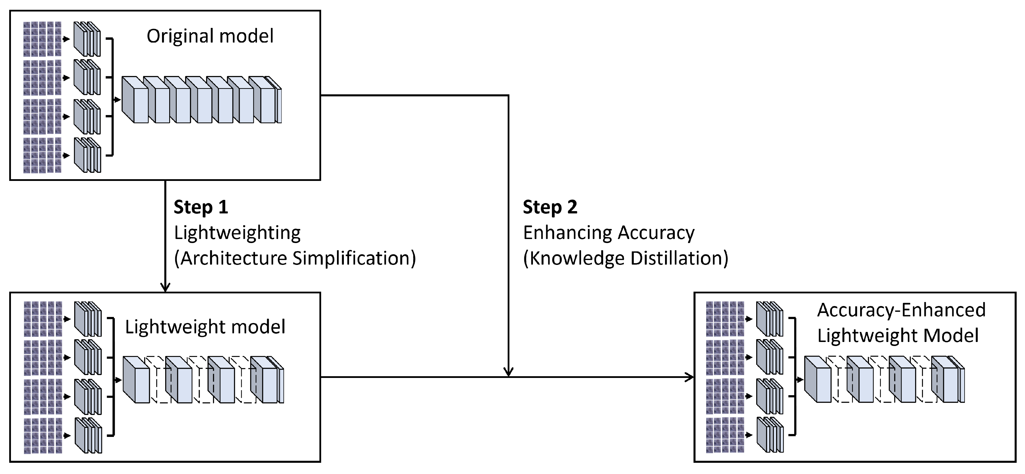
This study introduces a methodology that fundamentally incorporates two critical phases: lightweighting and accuracy enhancement. This approach is designed to reduce computational demands while simultaneously ensuring the maintenance or improvement of model precision, as illustrated in
Figure 1.
Lightweight Design
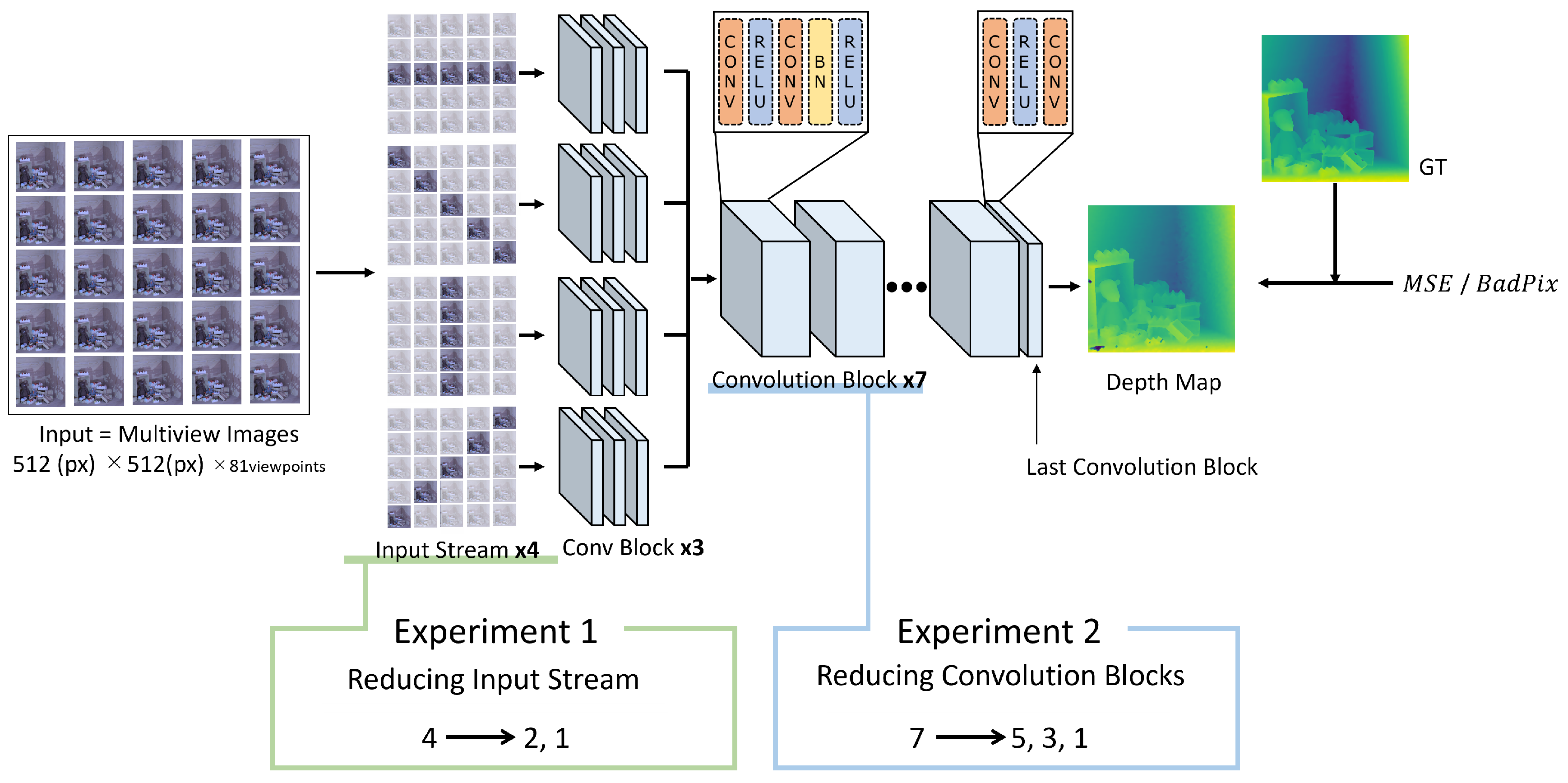
In the initial phase, our exploration focused on modifications to the model’s architecture. This process included making adjustments to the number of input streams and convolution blocks. These adjustments are expected to improve the model’s inference speed, leading to the development of a model that operates at higher speed with reduced parameters and computational cost. After training each adjusted model, the trade-off between inference speed and accuracy was quantitatively evaluated. Based on the obtained results, an optimized lightweight model was developed.
Accuracy Enhancement
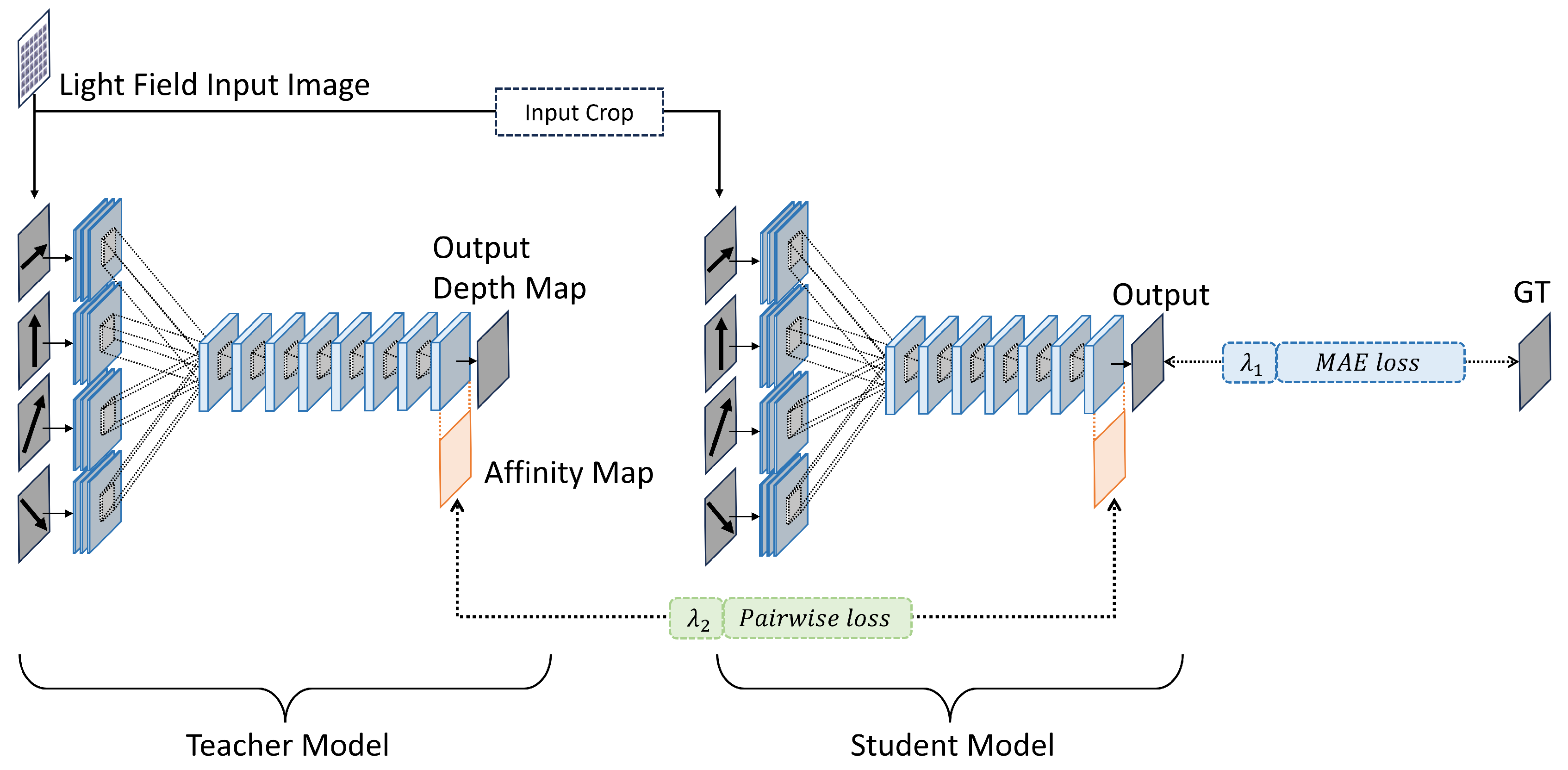
To address the precision loss incurred during the lightweighting process, the proposed feature-based offline knowledge distillation framework was adopted, as illustrated in
Figure 2. This method uses a more expressive and accurate original model as the teacher and the newly developed lightweight model as the student. Our framework significantly drew upon the research findings of Liu et al. [
26] and Wang et al. [
9] that focused on making depth prediction models simpler. The goal is to improve the student model’s accuracy by using the rich representational ability of the teacher model.
The lightweight student model and the teacher model typically differ in their network architectures such as the count of convolution layers. This difference leads to variations in the sizes of the final output depth maps between the two models. This discrepancy prevents a direct knowledge transfer between teacher and student models. To tackle this issue, our proposal includes a cropping process at the input stage to generate the output maps with identical size. This process enables the affinity maps comparison and knowledge transfer. To compare the affinity maps, two loss functions are utilized: pairwise loss and MAE (Mean Absolute Error) loss. The pairwise loss assesses the disparity between the teacher’s and student’s predictions, whereas the MAE loss measures the deviation of the student model’s output from the ground truth. During the training phase, the teacher model’s parameters are kept constant. In contrast, the student model’s parameters undergo updates to achieve optimal performance.
Loss Functions
In order to transfer feature-based knowledge during offline distillation, affinity maps are generated, which help capture and mirror important features from the teacher model. For a specific layer of a given model, the feature map
was considered, where
W and
H denote the width and height of the feature maps, respectively, and
C represents the number of channels. The cosine similarity between feature vectors at each pixel is calculated as the pairwise angular distance which can be denoted by
As learning progresses, the loss function is designed such that the pairwise angular distance of the student model approaches that of the teacher model. The relationship is as follows,
Here,
denotes the set of feature maps from the student model and
represents the set from the teacher model. Subsequently, an affinity map is constructed. This map is formed by calculating the pairwise angular distance for each pixel. Each pixel’s entry in the map represents this distance. This method effectively encodes the spatial relationships between pixels. First, for the purpose of subsequent processing, the feature map FF is reshaped and flattened as follows:
Using this flattened feature map
, the element of affinity map
can be written by,
In this equation,
represent the coordinates in the affinity maps, indicating the position of each pixel with respect to one another. The index
k runs along the channel dimension, serving as an iterator through the feature maps’ depth. The expression
calculates the affinity between pixels at positions
i and
j by summing the product of their values across all channels
C, normalized by the square of the total number of elements in the feature map, which is the product of the width
W and height
H of the feature map. This normalization accounts for the size of the feature map, ensuring that the affinity value is scaled appropriately. By comparing the affinity maps from the teacher model and the student model, the similarity between them can be quantified as the distillation loss
,
Here,
denotes the normalization constant and
and
respectively represent the affinity maps of the student and teacher models. Additionally, the inference accuracy of the student model is evaluated using MAE. This is calculated by comparing the output depth map from the student model
with the ground truth
. The loss function is defined as:
The total loss function
employed during the training phase is computed by incorporating fixed parameters
and
, and it is given by the following expression:
4. Experimental Setup
Lightweighting Experiments
Simplification by Reducing Convolution Blocks
In order to investigate the impact of varying the number of convolution blocks, four models were developed: the original model with seven convolution blocks, and lightweight variants with five, three, and one block(s), respectively. The configuration of each model in terms of the number of convolution blocks is summarized in
Table 1. This approach enables a direct comparison of model performance relative to the structural complexity.
4.1. Accuracy Enhancement Experiments
Limits of Model Disparity between Teacher and Student
The experiment was designed to determine the permissible differences in architecture and expressive power between the teacher and student models during knowledge distillation. For the purpose of constructing an accuracy enhancement framework, student models with a reduced number of convolution blocks were selected as minimal lightweight models. Specifically, student models with one and three convolution blocks removed were employed for comparison, as detailed in the architectural configurations outlined in
Table 2. The models were trained with a batch size of 16,
and
empirically fixed at 0.6, and a learning rate consistently set at
. Despite varying the learning rate scheduling as indicated by Shin et al. [
11] and Hassan et al. [
12], differential convergence rates across lightweight models in knowledge distillation posed comparison challenges. Therefore, a fixed learning rate of
was adopted, as it enabled the model to converge more quickly and achieve the lowest possible loss value. During the training phase, the dataset was utilized not as whole images but as patches as utilized in Shin et al. [
11]. These patches had sizes of 25×25 for the teacher model, 23×23 for the student model with one block removed, and 19×19 for the student model with three blocks removed. After training in the proposed knowledge distillation framework, each student model was deployed independently from the teacher model for depth estimation on the test dataset. The accuracy of the student models was quantified using MSE and BadPix metrics. Each student model has different capacities due to the varying number of convolution blocks: one and three removed, respectively. To highlight the effect of knowledge distillation, each student model trained in knowledge distillation was compared with the respective model trained from scratch.
The Evaluation of Optimal Knowledge Position
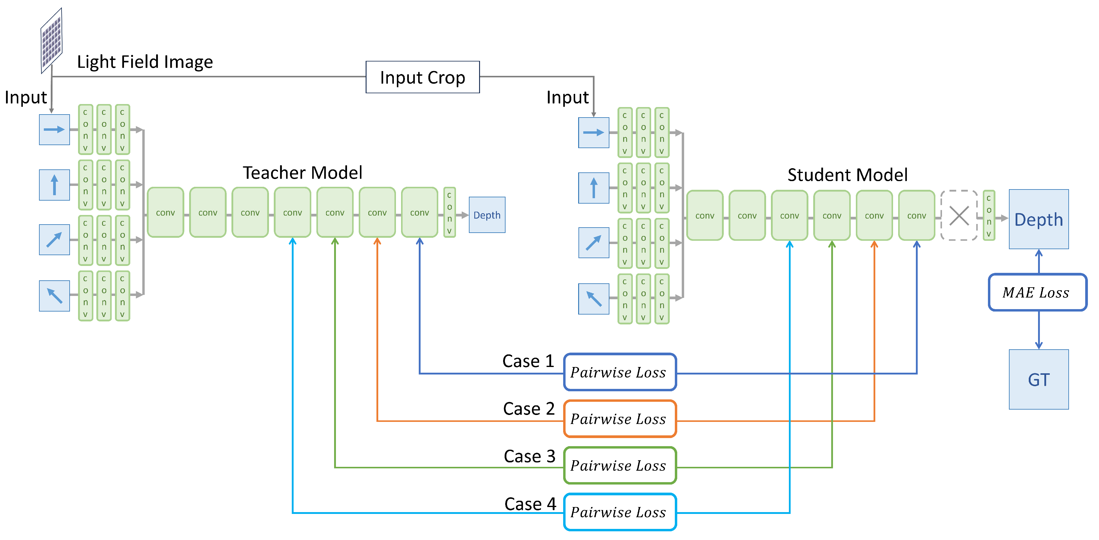
To identify the optimal convolution block position for proposed knowledge distillation, four different student models were compared. Under identical conditions and using the same teacher model, the experiments varied only the convolution layer location used for generating the affinity map, as illustrated in
Figure 4. Affinity maps were generated using feature maps from the second layer of four specific convolution block positions: the last, the second-to-last, the third-to-last, and the fourth-to-last blocks as summarized in the
Table 3. The reason for selecting these blocks is detailed in Chapter
Section 5, where our visualization study revealed that meaningful features for depth estimation start to emerge from the fourth block from the end, equivalently the third block from the start. Consequently, this experiment utilized only the blocks beyond this critical fourth block. The batch size, parameters
and
, and the learning rate were the same as in the previous experiment. After training, each student model was independently evaluated for inference performance on the test dataset. The performance of knowledge transferred from specific convolution blocks was assessed using MSE and BadPix metrics. This evaluation aimed to determine which knowledge transfer position minimized these metrics, thereby establishing a ranking of effectiveness among the convolution blocks.
5. Results
Lightweighting Experiments
Simplification by Reducing Convolution Blocks
In the experiments, we evaluated the impact of simplification on inference speed and accuracy by reducing the number of convolution blocks within EPINET.
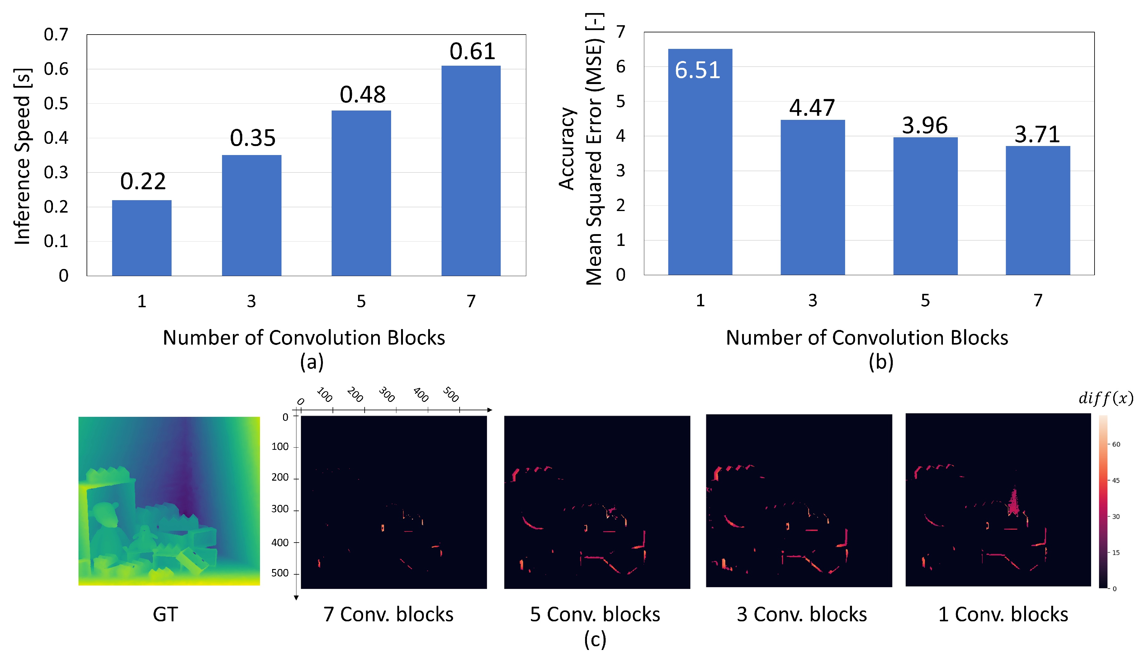
Figure 6a demonstrates that the inference speed changes linearly with the number of convolution blocks. This linear change is primarily attributed to the fact that computational complexity is roughly proportional to the number of convolution blocks. In contrast, a notable difference in inference accuracy was observed between models with three convolution blocks and those with only one block, as demonstrated in
Figure 6b. Furthermore, the visualization in
Figure 6c reveals that the model with a single convolution block produces a significant number of planar errors.
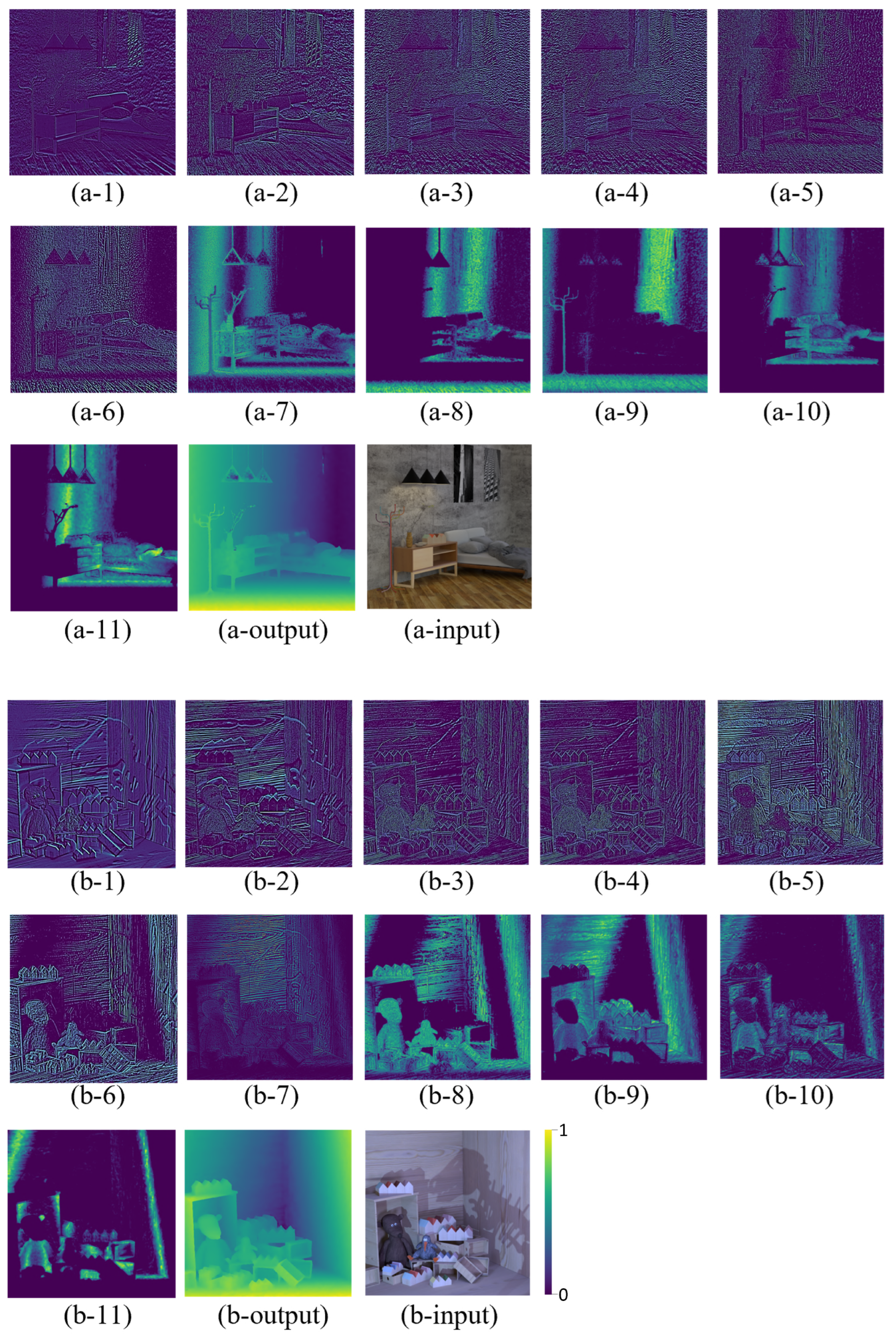
In order to identify the factors contributing to the significant decrease in accuracy observed in the single convolution block model, we visualized the internal representations within EPINET and extracted feature maps to directly understand the depth prediction process.
Figure 7 demonstrates the first feature maps in each convolution block. It became clear that contour information was captured up to the second block (a/b-6), whereas the third block (a/b-7) and subsequent ones were responsible for extracting fill and planar information. Considering that depth estimation relies on the generation of continuous and planar maps, the significance of planar information cannot be overstated. This realization led to the insight that at least three convolution blocks are necessary to capture this critical information. This finding explains the observed significant decrease in accuracy for the model with a single convolution block, highlighting how the presence of three convolution blocks contributes significantly to capturing depth information effectively, compared to a model with only one block. Consequently, this analysis indicates the importance of internal information processing in determining the lightweighting approach.
5.1. Accuracy Enhancement Experiments
The Evaluation of the Limits of Model Disparity between Teacher and Student
To design a knowledge distillation framework, adapting the optimal student model is a key step. Cho et al. [
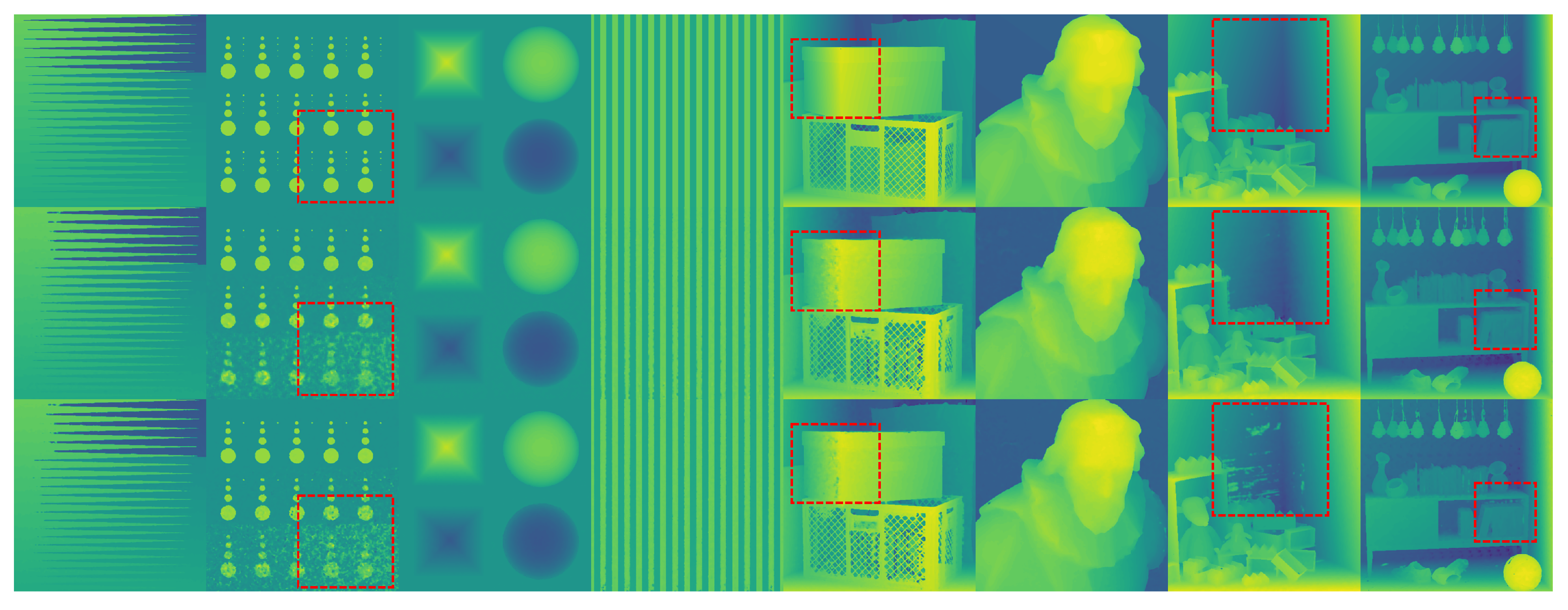
29] indicated that when there is a large disparity in representation power between the teacher model and the student model, knowledge transfer is ineffective. In order to explore the extent of the difference that can be tolerated between teacher and student models in knowledge distillation, two variations of the student model were tested: one with a single convolution block removed, referred to as the ’compact model’, and another with three convolution blocks removed, referred to as the ’ultra-compact model’. Using these lightweight student models and the same teacher model, the students were trained through the knowledge distillation framework. Subsequently, they were evaluated to assess the effectiveness of the training. The accuracy results of each model are presented in
Table 4 and visualized in
Figure 8.
From these results, it was observed that while the compact model showed improvements in both MSE and BadPix through knowledge distillation, the ultra-compact model, on the other hand, experienced a decrease in accuracy. This indicates that in the case of the EPINET architecture, knowledge distillation does not work effectively for enhancing the accuracy when there is a difference of three convolution blocks between the teacher and student models. In other words, it was found that the acceptable difference in convolution blocks is less than three. To investigate how the difference of three convolution blocks influences the effectiveness of knowledge distillation, an examination of the accuracy trends over epochs was conducted.
Figure 9 illustrates the change in accuracy measured with BadPix for both the compact model and the ultra-compact model. Unlike the compact model, the ultra-compact model demonstrated a decline in performance after 7500 epochs. That is, the student model, with three convolutional blocks removed, ceased to improve its accuracy at an early stage. These findings indicate that the large model discrepancy between the student and teacher models likely made it difficult for the student model to appropriately learn the abundant information held by the teacher model. As a result, the learning progression adapted in an overly specific manner to the features or mechanisms of the teacher model. This is considered a form of overfitting, resulting in decreased generalization ability.
The Evaluation of Knowledge Location
To investigate the optimal knowledge location for transfer within the proposed method, four different scenarios with varying knowledge locations were experimented with, and the accuracy results were compared using MSE and BadPix.
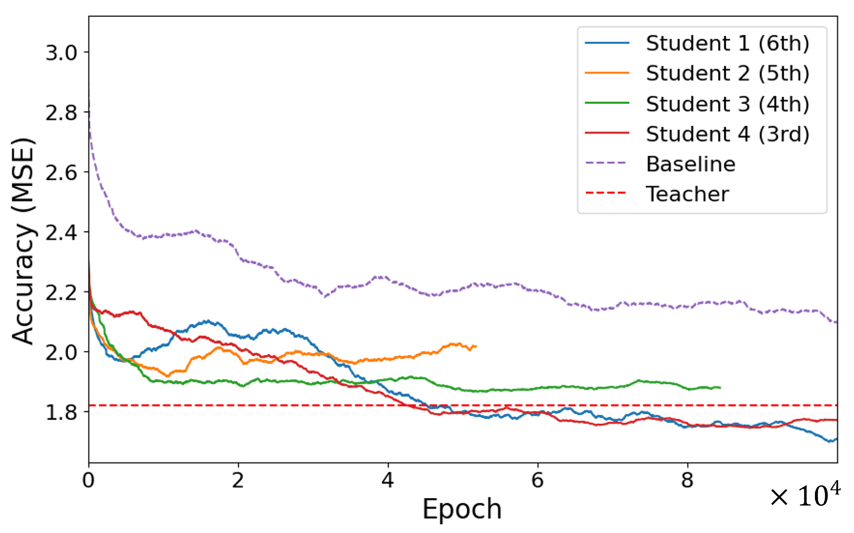
Figure 10 illustrates the change in MSE across four knowledge locations with colored solid lines, where the purple dotted lines indicate the accuracy of the baseline model trained from scratch without utilizing the proposed method. The model represented in Orange was discontinued as it failed to demonstrate further accuracy improvement, and all student models were trained up to
epochs.
The results revealed that all student models trained within the proposed method exhibited better MSE accuracy than the baseline, regardless of the knowledge position imitated through knowledge distillation. This indicates that student models learned more accurately within the framework of the proposed method than when trained independently, underscoring the effectiveness of the method. Moreover, learning tendencies varied significantly based on the knowledge position, especially for student models that mimicked the knowledge from the third (Red) and sixth blocks (Blue). These models consistently updated the accuracy beyond that of the teacher model, suggesting that optimal knowledge transfer can potentially enhance accuracy to surpass that of the teacher model. Considering the two knowledge locations that surpassed the accuracy of the teacher model, the distinct advantage observed with the knowledge from the third block (Red) was linked to the extraction of critical advanced information pertinent to depth from this block. This implies that emulating the early-stage feature extraction approach facilitates efficient learning progress. In contrast, the advantage of the knowledge position of the last block (Blue) is likely due to its direct connection to depth information, which, when transferred, gives the student model knowledge that directly helps with depth estimation tasks.
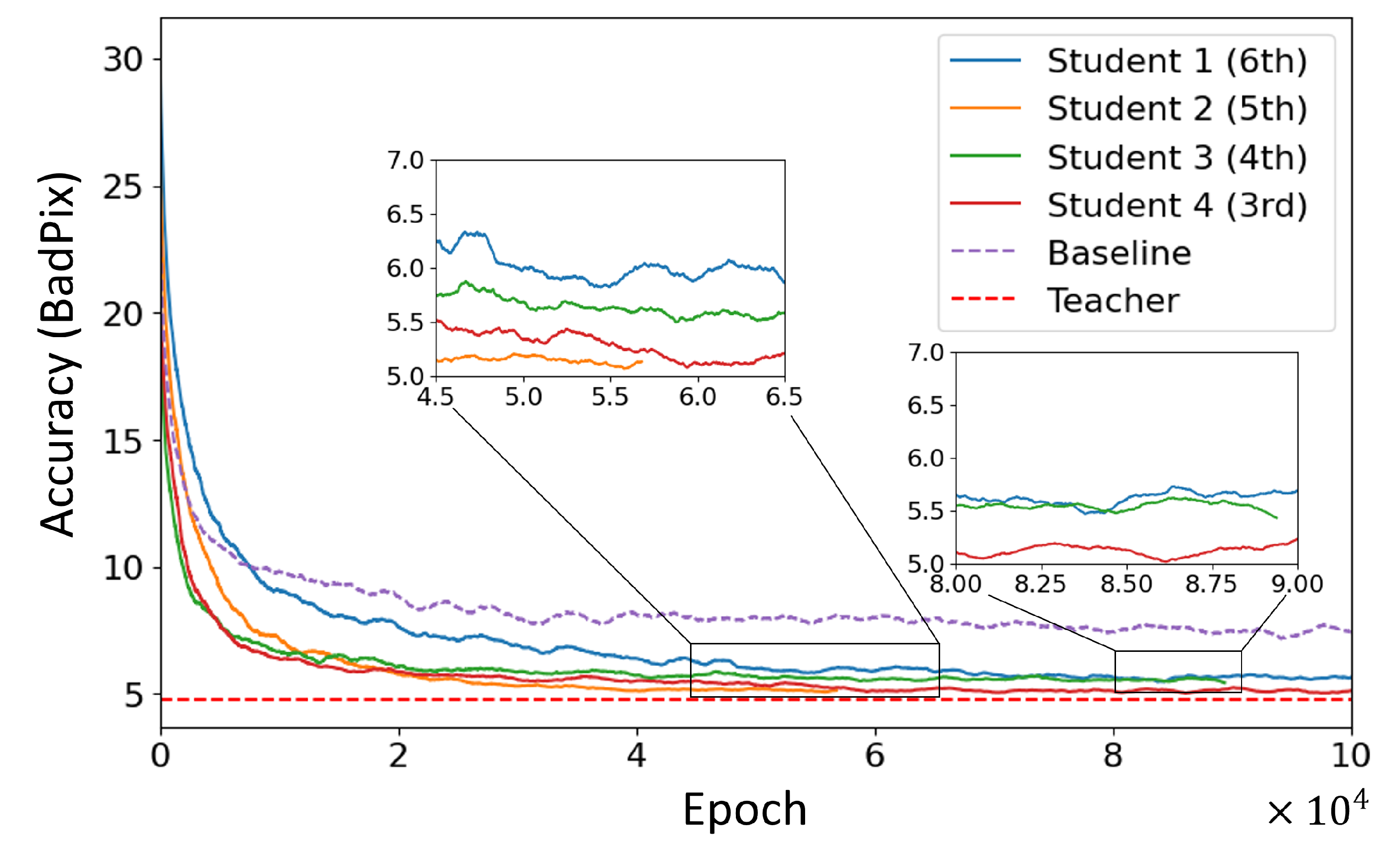
Figure 11 shows the BadPix accuracy change along training, where solid color lines correspond to the student models with different knowledge location transferring within the proposed method, and purple and red dotted lines mean the baseline model trained from scratch and the teacher model, respectively. Similar to MSE, all student models (Solid lines) imitating any knowledge position through the proposed method were more accurate than when learned solo (Purple dotted line), demonstrating the effectiveness of the proposed method using BadPix as a metric. It was also found that the superiority of knowledge positions differed between MSE and BadPix. In other words, although the Red and Blue models exhibited high accuracy in MSE, it was the Orange and Red models that showed high performance in BadPix.
Given the distinct tasks evaluated by MSE and BadPix—with MSE assessing overall error and BadPix focusing on significant errors—it was observed that the effectiveness of specific knowledge locations varies between these metrics. This variation highlights the task-specific nature of knowledge transfer, suggesting that no single knowledge location universally optimizes all aspects of model performance during compression. Instead, selecting an appropriate knowledge location must consider the particular goals, whether minimizing overall error or reducing significant errors.
Furthermore, the results revealed that surpassing the teacher model’s accuracy with BadPix proved consistently challenging, pointing to the nuanced challenge of optimizing for different error measurements. This emphasizes that the success of knowledge transfer depends significantly on the task, reinforcing the need to tailor the approach based on the specific requirements of the task at hand.
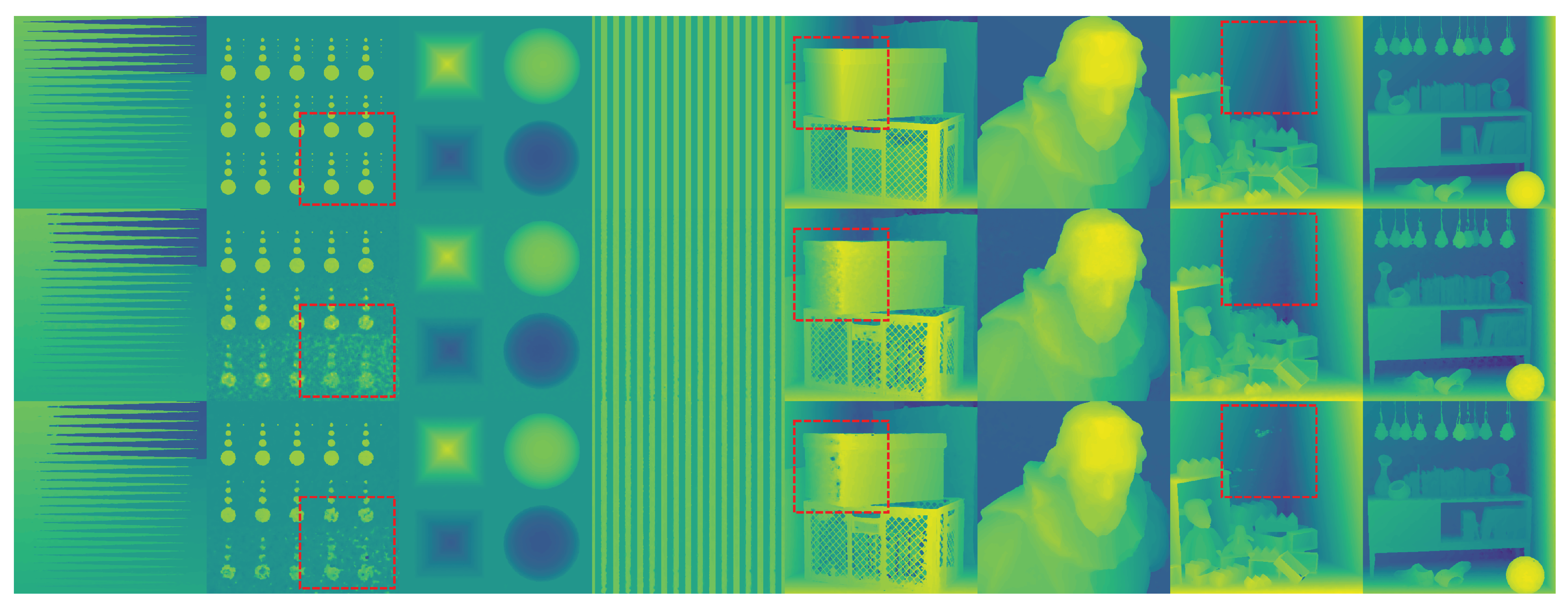
Figure 12 clearly illustrates the disparity in prediction accuracy between models trained with the proposed knowledge distillation method and those trained entirely from scratch. Our proposed method is shown to reduce planar errors, which are highlighted in red. Since depth estimation models generally require planar features, minimizing planar errors is crucial for the performance of depth estimation algorithms.
6. Conclusion
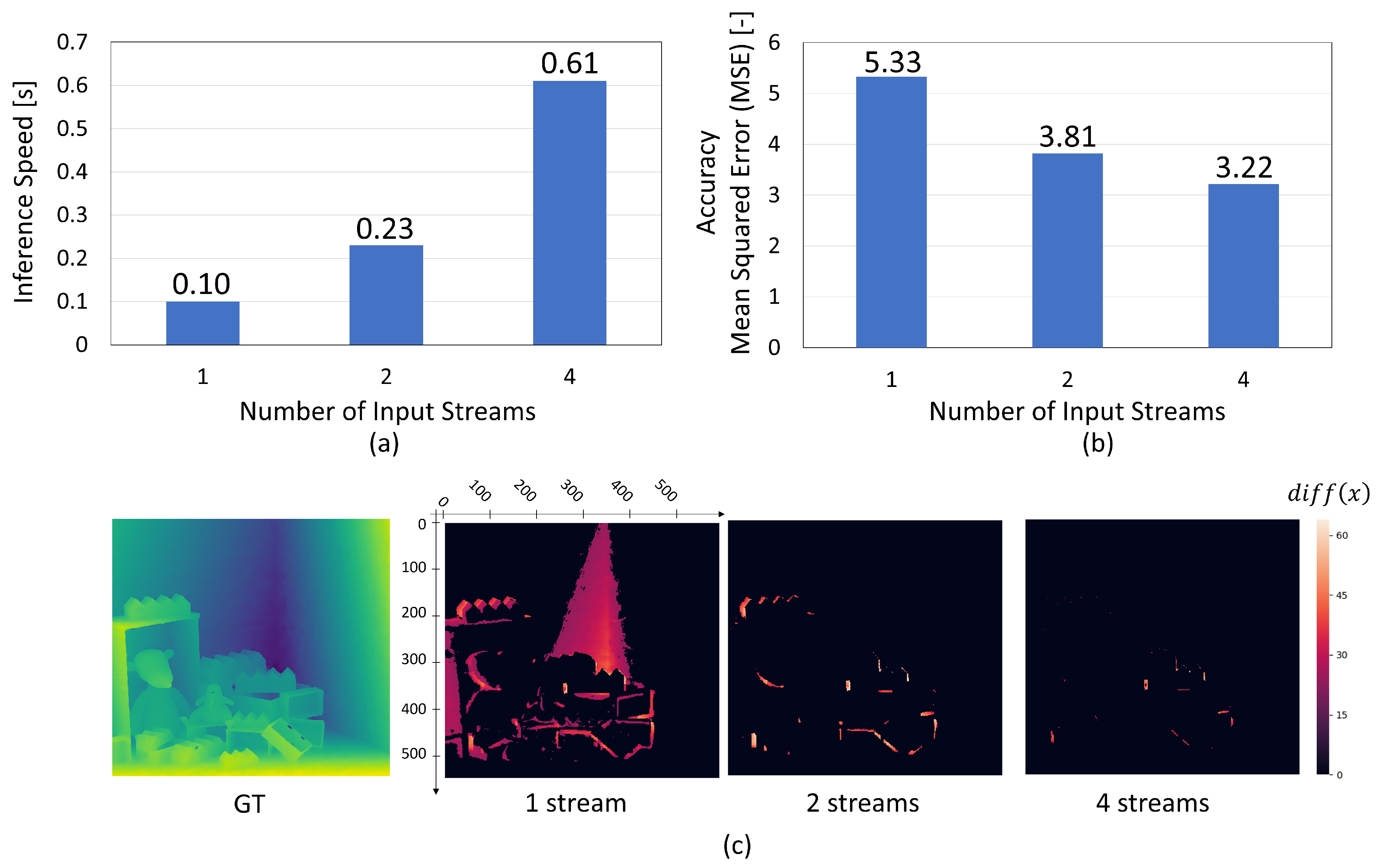
In this study, we developed a methodology that reduces the computational load of light field depth estimation models without notably compromising accuracy. Unlike existing methods that typically struggle to balance model lightening with precision enhancement, our approach provides a compelling solution. The experimentation involved the strategic reduction of input stream numbers and convolution block counts, which allowed us to evaluate the trade-offs between inference speed and accuracy quantitatively. Through the use of MSE and BadPix metrics, we observed that processing speed improved linearly with reductions in input streams and convolution operations. However, significant accuracy disparities were evident when comparing models with more than three convolution blocks to those with fewer. These observations served as guidelines for creating a lightweight model, which was then utilized as the student model in the next steps.
Further into our study, we embarked on enhancing the precision of our models through the deployment of a knowledge distillation framework. A lightweight model was used as the student model, with the baseline model functioning as the teacher. This setup employed a pairwise loss for affinity map comparisons and an MAE loss to quantify discrepancies between the student model’s output and the ground truth. By feeding cropped images, we ensured alignment of output domains. This enabled our framework to support successful knowledge imitation across networks with differing numbers of convolution blocks. The framework facilitated the evaluation of the permissible range of discrepancies between teacher and student models and allowed for the experimentation on optimal knowledge mimicry positions within the models. Interestingly, our findings also revealed that the reduction of three convolution blocks could detrimentally affect the effectiveness of knowledge distillation. Moreover, the differential advantages of mimicking specific knowledge positions suggested that the superiority of specific knowledge positions and the task dependency of knowledge location are critical factors in the effectiveness of knowledge distillation techniques.
As a result, our research achieved a balanced enhancement in both the speed and accuracy of depth estimation models. The implementation of our methodology resulted in models that were 1.2 times faster and exhibited a 1.1-fold improvement in MSE accuracy. These results affirm the potential of our approach in simultaneously achieving model lightweighting and precision enhancement.
This study significantly demonstrates that employing enhanced student models as teachers in subsequent knowledge distillation cycles can lead to improved model performance through iterative refinement. This approach strives for continuous improvements while maintaining minimal differences between teacher and student models, with a discrepancy of fewer than three convolution blocks in our experiments. Although the progress in each cycle may be modest, the cumulative effect of these enhancements can substantially boost the speed and accuracy of depth estimation models, underscoring the importance of ongoing optimization in achieving superior computing performance.
Acknowledgments
This work was supported by MEXT KAKENHI Grant Number JP22569332.
References
- Ulusoy, U.; Eren, O.; Demirhan, A. Development of an obstacle avoiding autonomous vehicle by using stereo depth estimation and artificial intelligence based semantic segmentation. Engineering Applications of Artificial Intelligence 2023, 126, 106808.
- Miclea, V.C.; Nedevschi, S. Monocular Depth Estimation With Improved Long-Range Accuracy for UAV Environment Perception. IEEE Transactions on Geoscience and Remote Sensing 2022, 60.
- Xiong, J.; Hsiang, E.L.; He, Z.; Zhan, T.; Wu, S.T. Augmented reality and virtual reality displays: emerging technologies and future perspectives. Light: Science & Applications 2021, 10, 1–30.
- Pilzer, A.; Lathuiliere, S.; Sebe, N.; Ricci, E. Refine and distill: Exploiting cycle-inconsistency and knowledge distillation for unsupervised monocular depth estimation. Proceedings of the IEEE/CVF Conference on Computer Vision and Pattern Recognition, 2019, pp. 9768–9777.
- Chen, X.; Ma, H.; Wan, J.; Li, B.; Xia, T. Multi-view 3d object detection network for autonomous driving. Proceedings of the IEEE conference on Computer Vision and Pattern Recognition, 2017, pp. 1907–1915.
- Hazirbas, C.; Ma, L.; Domokos, C.; Cremers, D. Fusenet: Incorporating depth into semantic segmentation via fusion-based cnn architecture. Computer Vision–ACCV 2016: 13th Asian Conference on Computer Vision, Taipei, Taiwan, November 20-24, 2016, Revised Selected Papers, Part I 13. Springer, 2017, pp. 213–228.
- Shotton, J.; Fitzgibbon, A.; Cook, M.; Sharp, T.; Finocchio, M.; Moore, R.; Kipman, A.; Blake, A. Real-time human pose recognition in parts from single depth images. CVPR 2011. Ieee, 2011, pp. 1297–1304.
- Howard, A.G.; Zhu, M.; Chen, B.; Kalenichenko, D.; Wang, W.; Weyand, T.; Andreetto, M.; Adam, H. Mobilenets: Efficient convolutional neural networks for mobile vision applications. arXiv preprint arXiv:1704.04861 2017.
- Wang, Y.; Li, X.; Shi, M.; Xian, K.; Cao, Z. Knowledge distillation for fast and accurate monocular depth estimation on mobile devices. Proceedings of the IEEE/CVF Conference on Computer Vision and Pattern Recognition, 2021, pp. 2457–2465.
- Ng, R.; Levoy, M.; Brédif, M.; Duval, G.; Horowitz, M.; Hanrahan, P. Light field photography with a hand-held plenoptic camera. PhD thesis, Stanford university, 2005.
- Shin, C.; Jeon, H.G.; Yoon, Y.; Kweon, I.S.; Kim, S.J. EPINET: A Fully-Convolutional Neural Network Using Epipolar Geometry for Depth from Light Field Images. CVPR. Computer Vision Foundation, 2018. Available: IEEE Xplore.
- Hassan, A.; Sjöström, M.; Zhang, T.; Egiazarian, K. Light-weight epinet architecture for fast light field disparity estimation. 2022 IEEE 24th International Workshop on Multimedia Signal Processing (MMSP). IEEE, 2022, pp. 1–5.
- Richter, M.L.; Schöning, J.; Wiedenroth, A.; Krumnack, U. Should You Go Deeper? Optimizing Convolutional Neural Network Architectures without Training. arXiv preprint arXiv:2106.12307 2021.
- Adelson, E.H.; Wang, J.Y. Single lens stereo with a plenoptic camera. IEEE transactions on pattern analysis and machine intelligence 1992, 14, 99–106.
- Wang, Y.; Wang, L.; Wu, G.; Yang, J.; An, W.; Yu, J.; Guo, Y. Disentangling Light Fields for Super-Resolution and Disparity Estimation. Proceedings of the IEEE/CVF Conference on Computer Vision and Pattern Recognition. College of Electronic Science and Technology, National University of Defense Technology; State Key Laboratory of Synthetical Automation for Process Industries, Northeastern University; School of Information Science and Technology, ShanghaiTech University, 2019.
- Vizcaino, J.P.; Wang, Z.; Symvoulidis, P.; Favaro, P.; Guner-Ataman, B.; Boyden, E.S.; Lasser, T. Real-time light field 3D microscopy via sparsity-driven learned deconvolution. 2021 IEEE International Conference on Computational Photography (ICCP). IEEE, 2021, pp. 1–11.
- Jeon, H.G.; Park, J.; Choe, G.; Park, J.; Bok, Y.; Tai, Y.W.; Kweon, I.S. Accurate Depth Map Estimation from a Lenslet Light Field Camera. Proceedings of the IEEE/CVF Conference on Computer Vision and Pattern Recognition. Korea Advanced Institute of Science and Technology (KAIST), Republic of Korea, 2015.
- Wang, T.C.; Zhu, J.Y.; Hiroaki, E.; Chandraker, M.; Efros, A.A.; Ramamoorthi, R. A 4D Light-Field Dataset and CNN Architectures for Material Recognition. European Conference on Computer Vision. Springer, 2016, pp. 121–138.
- Li, J.; Lu, M.; Li, Z.N. Continuous Depth Map Reconstruction From Light Fields. IEEE Transactions on Image Processing 2015, 24, 3257–3265.
- Sheng, H.; Liu, Y.; Yu, J.; Wu, G.; Xiong, W.; Cong, R.; Chen, R.; Guo, L.; Xie, Y.; Zhang, S.; others. LFNAT 2023 Challenge on Light Field Depth Estimation: Methods and Results. Proceedings of the CVPR Workshop. Computer Vision Foundation, 2023.
- Miya, R.; Kawaguchi, T.; Saito, T. Real-time depth estimation machine learning model for Light Field raw images. The 17th Asian Symposium on Visualization, 2023.
- Hinton, G.; Vinyals, O.; Dean, J. Distilling the Knowledge in a Neural Network. arXiv preprint arXiv:1503.02531 2015.
- He, Y.; Zhang, X.; Sun, J. Channel Pruning for Accelerating Very Deep Neural Networks. International Conference on Computer Vision (ICCV). IEEE, 2017. Available: Computer Vision Foundation open access.
- Polino, A.; Pascanu, R.; Alistarh, D. Model Compression via Distillation and Quantization. International Conference on Learning Representations. ICLR, 2018.
- Gou, J.; Yu, B.; Maybank, S.J.; Tao, D. Knowledge Distillation: A Survey. arXiv preprint arXiv:2006.05525 2020. Accepted for publication in International Journal of Computer Vision (2021).
- Liu, Y.; Shun, C.; Wang, J.; Shen, C. Structured knowledge distillation for dense prediction. arXiv preprint arXiv:1903.04197 2019.
- Li, Z.; Yang, B.; Yin, P.; Qi, Y.; Xin, J. Feature Affinity Assisted Knowledge Distillation and Quantization of Deep Neural Networks on Label-Free Data. arXiv preprint arXiv:2308.02023 2023. Available: arXiv.org.
- Honauer, K.; Johannsen, O.; Kondermann, D.; Goldluecke, B. A Dataset and Evaluation Methodology for Depth Estimation on 4D Light Fields. Proceedings of the Asian Conference on Computer Vision (ACCV). HCI, Heidelberg University; University of Konstanz, 2016.
- Cho, J.H.; Hariharan, B. On the Efficacy of Knowledge Distillation. Proceedings of the IEEE/CVF International Conference on Computer Vision (ICCV); IEEE, , 2019.
Figure 1.
Illustration of Two-step Optimization Framework. First, the model is simplified for enhanced speed and compactness. This simplification accelerates the inference speed but also leads to reduced accuracy. Then, through offline knowledge distillation with the original model as the teacher and the simplified model as the student, accuracy is effectively restored without compromising efficiency.
Figure 2.
Framework for Enhancing the Accuracy of a Lightweight Model Using Offline Knowledge Distillation. GT denotes Ground Truth, the label data for the input images, which is referred to during the training stage. Although the same images are input to both the teacher and student models, the student model receives cropped versions to ensure the final depth maps align over the same areas. The loss function incorporates both pairwise loss from affinity maps and Mean Absolute Error (MAE) loss.
Figure 3.
Overview of the Simplification Experiments on the EPINET Architecture. This diagram illustrates which parts of the architecture were reduced, specifically targeting reductions in input streams and convolution blocks to measure inference accuracy and speed.
Figure 3.
Overview of the Simplification Experiments on the EPINET Architecture. This diagram illustrates which parts of the architecture were reduced, specifically targeting reductions in input streams and convolution blocks to measure inference accuracy and speed.
Figure 4.
Overview of Experiments on Optimal Knowledge Position Evaluation. Four scenarios with varied hint layer positions were assessed for inference accuracy, measured using MSE and BadPix.
Figure 4.
Overview of Experiments on Optimal Knowledge Position Evaluation. Four scenarios with varied hint layer positions were assessed for inference accuracy, measured using MSE and BadPix.
Figure 5.
Input Stream Reduction Analysis: (a,b) Exploring the Relationship between the Number of Input Streams and Inference Speed/Accuracy. (c) Visualization of BadPix Differences. Models compared include 1 stream (), 2 streams (, ), and 4 streams (, , , ), highlighting significant error spread variations.
Figure 6.
Convolution Block Reduction Analysis: (a,b) Relationship between the Number of Convolution Blocks and Inference Speed/Accuracy. (c) Visualization of BadPix Variation. Reducing blocks to fewer than three increases errors related to coverage.
Figure 6.
Convolution Block Reduction Analysis: (a,b) Relationship between the Number of Convolution Blocks and Inference Speed/Accuracy. (c) Visualization of BadPix Variation. Reducing blocks to fewer than three increases errors related to coverage.
Figure 7.
Hidden Layer Visualization of EPINET. The internal representations are illustrated with two different scenes, described as (a) and (b), representing "Bicycle" and "Dino" in the 4D dataset [
28], with corresponding inputs labeled as (a/b-input). The color within the images indicates that each pixel feature is activated, moving from dark blue to yellow. Images (a/b-1) to (a/b-4) are from input-stream convolution blocks, while (a/b-5) to (a/b-11) are from reduced concatenated blocks. The clarity in images (a/b-1)-(a/b-6) is enhanced to underline characteristics, with layers (a/b-5) and (a/b-6) indicating a focus on edge extraction. From images (a/b-7) onwards, planar information begins to be extracted, corresponding to the third convolution block, highlighting the transition from edge to planar feature extraction.
Figure 8.
Comparison of Ground Truth (Top) With Predictions From Models With Different Convolution Block Configurations. The models compared include one with three blocks removed (middle) and another with one block removed (bottom). Red Square Areas Highlight the Significant Difference in Error Distribution Between the Compact Model and Ultra-Compact Model. Inference was conducted on the light field synthetic dataset [
28].
Figure 9.
Comparison of BadPix Accuracy Improvement over Training Epochs between the Compact (left) and Ultra-compact Models (right). For the purpose of comparing accuracy trends, BadPix values are normalized, and the epoch range is shown up to 17,500 epochs.
Figure 9.
Comparison of BadPix Accuracy Improvement over Training Epochs between the Compact (left) and Ultra-compact Models (right). For the purpose of comparing accuracy trends, BadPix values are normalized, and the epoch range is shown up to 17,500 epochs.
Figure 10.
MSE Performance Comparison Across Student Models With Different Knowledge Transfer Locations. Solid lines represent the student models, each showcasing performance with different locations for knowledge transfer. The baseline model is depicted with a dotted purple line, and the teacher model with a dotted red line. The student models and the baseline model are plotted with a moving average, taken over 700 epochs, to smooth out fluctuations and provide a clearer view of trends.
Figure 11.
BadPix Accuracy Comparison Among Student Models at Different Knowledge Locations. Solid lines represent the student models, each evaluated at various knowledge transfer locations. The Baseline Model is depicted with a dotted purple line, and the Teacher Model with a dotted red line. All student models and the baseline model are plotted with a moving average, taken over 700 epochs, to facilitate a clearer comparison of trends.
Figure 12.
Comparison of Ground Truth (Top) With Depth Maps Estimated by Models. Models trained with (middle) and without (bottom) the proposed framework are compared, illustrating our method’s effectiveness. The Light Field Synthetic Dataset from Honauer et al. [
28] was used for testing. Red areas in each image highlight significant differences in error distribution between the student model and the baseline model.
Table 1.
Model Configurations with Varied Number of Convolution Blocks
Table 1.
Model Configurations with Varied Number of Convolution Blocks
| Model |
Number of Convolution Blocks |
| Baseline Model |
7 |
| Lightweight Model 1 |
5 |
| Lightweight Model 2 |
3 |
| Lightweight Model 3 |
1 |
Table 2.
Architectural Configurations of Teacher and Student Models
Table 2.
Architectural Configurations of Teacher and Student Models
| Scenario |
Input Size |
Number of Convolution Blocks |
| |
Teacher |
Student |
Teacher |
Student |
| 1 |
25×25 |
23×23 |
7 |
6 |
| 2 |
25×25 |
19×19 |
7 |
4 |
Table 3.
Comparison of Knowledge Transfer Locations within Convolution Blocks. Specified knowledge was transferred among the teacher and student models in the offline knowledge distillation framework.
Table 3.
Comparison of Knowledge Transfer Locations within Convolution Blocks. Specified knowledge was transferred among the teacher and student models in the offline knowledge distillation framework.
| Scenario |
Position of Transferred Knowledge |
| |
Teacher |
Student |
| 1 |
7th |
6th |
| 2 |
6th |
5th |
| 3 |
5th |
4th |
| 4 |
4th |
3rd |
Table 4.
Comparison of Best MSE and Best BadPix Between Models. Green indicates an improvement in accuracy, while red indicates a decrease in accuracy.
Table 4.
Comparison of Best MSE and Best BadPix Between Models. Green indicates an improvement in accuracy, while red indicates a decrease in accuracy.
| |
Student Model |
| |
Compact |
Ultra-compact |
| Best MSE |
1.71 ⟶ 1.41
|
1.73 ⟶ 1.84
|
| Best BadPix |
5.31 ⟶ 4.67
|
7.43 ⟶ 8.16
|
| lower is better |
|
|
Table 5.
Comparison Of Peak Performance Metrics Across Different Student Models. Varying in hint layer positions, these models are compared against the teacher and baseline models. Red text highlights the best performance within the student models for each metric, showcasing the impact of hint layer positioning on accuracy and error rates.
| Model |
Hint Layer Position |
Best MSE |
Best BadPix |
Runtine[ms] |
| Teacher |
- |
1.56 |
4.41 |
610 |
| Student Baseline |
- |
1.71 |
5.32 |
545 |
| Student Lightweight1 |
6th |
1.41 |
4.67 |
545 |
| Student Lightweight2 |
5th |
1.44 |
4.45 |
545 |
| Student Lightweight3 |
4th |
1.51 |
4.73 |
545 |
| Student Lightweight4 |
3rd |
1.51 |
4.37 |
545 |
| |
|
lower is better |
lower is better |
|
Disclaimer/Publisher’s Note: The statements, opinions and data contained in all publications are solely those of the individual author(s) and contributor(s) and not of MDPI and/or the editor(s). MDPI and/or the editor(s) disclaim responsibility for any injury to people or property resulting from any ideas, methods, instructions or products referred to in the content. |
© 2024 by the authors. Licensee MDPI, Basel, Switzerland. This article is an open access article distributed under the terms and conditions of the Creative Commons Attribution (CC BY) license (http://creativecommons.org/licenses/by/4.0/).
