Preprint
Article

Aging Renewal Point Processes and Exchangeability of Event Times

Altmetrics

Downloads

126

Views

49

Comments

0

A peer-reviewed article of this preprint also exists.

This version is not peer-reviewed

Submitted:

27 March 2024

Posted:

29 March 2024

You are already at the latest version

Alerts
Abstract
We investigate the impact of aging on exchangeable inter-arrival times in mixed renewal processes, exploring its implications for reliability and survival analysis. In this study, first, we revisit the definition of renewal point processes, where inter-event time intervals are considered as exchangeable non-negative random variables. Then, we define the concept of statistical aging as latency in the observational process of event counting. Latency affects event detection but preserves exchangeability. However, it may alter the statistical properties of inter-event time intervals. Our analytical and numerical assessments highlight the significance of aging in exchangeable lifetimes, offering insights into key metrics such as the failure survival function, renewal function, and hazard rate function. Through archetypal examples and empirical findings, we illustrate the implications of aging on renewal processes. In particular, employing a Bayesian perspective, we analyze high-frequency currency exchange rate data to assess the impact of aging on volatility risk evaluation. This study contributes novel insights to the literature of renewal theory and survival analysis, emphasizing the role of latency aging in stochastic point processes under exchangeability assumption.
Keywords: 
Subject: Computer Science and Mathematics  -   Applied Mathematics

1. Introduction

We numerically and analytically investigate the impact of aging on exchangeable inter-arrival times in mixed renewal processes. Renewal theory focuses on stochastic systems whose temporal evolution is punctuated by events called renewals. It has been extensively examined in seminal works [1,2,3] and is widely applied to reliability and survival analysis [4,5]. The theory does not need to specify the meaning or effect of single events, which is why renewal processes are at the core of many stochastic problems found in applied mathematics throughout many fields of science, engineering and economics [6,7].
The main purpose of this paper is to examine two important notions in the renewal theory of stochastic processes: the exchangeability property of inter-event times and the effect of aging on event counting. The notion of exchangeability was introduced by Bruno de Finetti [8,9]. Its significance is largely connected with "de Finetti’s representation theorem" and its generalized formulations, elucidating conditions connecting frequencies with subjective probabilities [9,10,11]. Within the framework of renewal theory for stochastic processes, exchangeability replaces the conventional assumption of observations being "independent and identically distributed with an unknown distribution," considering exchangeable observations as a sequence of conditionally independent and identically distributed (i.i.d.) random variables. A recently introduced class of renewal processes, named mixed renewal processes, have been based on exchangeability, reflecting indifference among distinct events in a point process [12,13,14]. In addition, we study statistical aging as a form of aging where there is a latency in event detection - the occurrence of an event momentarily "freezes" the detection process for a time t a , the age. This "freezing" generates waiting times which can potentially alter the statistical properties of the observed inter-event time intervals [15,16] . If such situation occurs, the correspondent point process is said to be affected by renewal aging defined by exchangeable lifetime intervals. However, we prove that if the original sequence of inter-event time intervals is exchangeable, observational latency preserves exchangeability of the new waiting-times. Aging has been investigated in the literature on stochastic processes [17,18], it is observed in various physical phenomena [19,20,21,22] and manifests in many complex dynamical systems [23,24]. In the field of quantitative finance, reliability and renewal theory are used in the study of market micro-structure models for the estimation of arrival times of trades or orders in financial markets [25,26,27,28]. At the same time, understanding the aging behavior of time series is fundamental to studies of the stability of financial markets [28,29,30]. As a case study, we analyze high-frequency data of exchange rates between currency pairs. By using a bayesian perspective on survival analysis, we observe that the aging, due to latency in recording the events, will alter the evaluation of volatility risk.
In Section 2, we remind the reader of some of the central concepts in reliability theory and survival analysis of renewal process under exchangeability assumption of inter-event time intervals. Later, in Section 3, we analytically assess the implications of aging on exchangeable lifetimes. We formulate aged versions of some key metrics in survival analysis of exchangeable renewal processes such as: the marginal distribution of waiting times (i.e., failure survival function), the average number of events (i.e., renewal function), and the rate of failure at any instant (hazard rate function). After the theoretical results, in Section 4, we discuss some archetypal examples of mixed renewal processes with intrinsic fluctuations of the underlying parameters due the fact that inter-arrival times between events may exhibit variability. We compare analytical and numerical results for some exchangeable mixture models where the effect of aging on the renewal process has some interesting implications for survival analysis. At the end of section, we present some empirical findings. As case study, we investigate high-frequency financial time series and, in particular, we use currency pairs with tick-by-tick historical exchange rates, treated as conditional observations on which we apply the survival analysis for exchangeable sequences. Finally, the discussion section will summarize the results obtained and highlight the novel contribution to the literature of renewal theory and reliability analysis in a subjective perspective.

2. Preliminaries

In this section we report some fundamental definitions and propositions on exchangeability of sequences of time-interval variables in renewal processes. Later we will frame such property in the field of renewal theory for point process with inter-event times which are exchangeable rather the independent and identically distributed (i.i.d.).
A sequence of inter-event time intervals is said to be exchangeable if the order of observations does not carry relevant information [10,31]. More precisely:
Definition 1. 
Let τ = { τ i : i N } a sequence of random variables defined over the probability space ( Ω , E , P ) , Where the sample space Ω = R > 0 , the event space E is a measurable subset of positive reals (namely a Borel set in R > 0 ), and the probability P is defined in terms of the cumulative distribution function.
A finite sequence of random variables ( τ 1 , , τ n ) is called exchangeable if n 2 ,
( τ 1 , τ 2 , , τ n ) = D ( τ σ ( 1 ) , τ σ ( 2 ) , , τ σ ( n ) ) σ S ( n )
where S ( n ) is the group of permutations of ( 1 , 2 , , n ) . If the sequence is infinite, it is said to be exchangeable if the finite collection ( τ 1 , , τ n ) are exchangeable for every finite n 1 or every permutation σ S
Let us notice that the equivalence in distribution, = D , simply means that the two proability distribution functions are the same. So the sequence takes values in a standard Borel space ( X , b ) where X is the positive reals and b is all of the Borel subsets of the positive reals. Exchangeability generalizes the notion of a sequence of random variables being independent and identically distributed (i.i.d.) and, in frequentist approach to statistics, observed data is assumed to be generated by a series of i.i.d. random variables with distribution parameterized by some unknown parameter which, on the contrary from a Bayesian perspective, it has some prior distribution, so the random variables which give the data are no longer independent. The representation theorem states that any infinite exchangeable sequence of random variables is a mixture of independent and identically distributed (i.i.d.) sequences, in the sense of the following proposition which covers the general case for real-valued exchangeable random quantities as in [11,32,33] known as generalized de Finetti’s theorem:
Proposition 1 
(representation theorem). Consider an infinitely exchangeable sequence { τ 1 , τ 2 , } , there exists a probability de Finetti’s measure μ over the space F of all distribution functions on R , such that the joint distribution function of the sequence has the form:
P ( τ 1 , τ 2 , , τ n ) = F i = 1 n F ( τ i ) d μ ( F ) where μ ( F ) = lim n P ( F n )
with μ is the probability distribution of the empirical random distribution F n defined by { τ 1 , τ 2 , , τ n } .
The previous proposition implies that we should proceed as if the observations { τ 1 , τ 2 , , τ n } are independent conditional on F, an unknown cumulative distribution (an infinite-dimensional parameter), with a belief distribution μ for F, having the operational interpretation in eq.(2) of what we believe the empirical distribution function would look like for a large sample. This means that infinite sequences of exchangeable random variables can be regarded equivalently as sequences of conditionally i.i.d. random variables, based on some underlying distributional form described by the de Finetti probability measure μ . Note that this equivalence does not quite hold for finite exchangeability. In the sense that there are finite exchangeable sequences which cannot be represented as a mixture of i.i.d. processes. However, they can be modeled as approximately being conditionally i.i.d. as shown in [34,35,36] under the condition that the sample size n k where k are the first outcomes of the sample of size n in a sampling scheme of drawing without replacement. In the trivial case, when the sequence is generated by a de Finetti mixture with a degenerate mixing distribution, i.e., when μ = δ F , with δ a denoting a unit point mass at a, then the sequence is (unconditionally) i.i.d. So, it is evident how the condition of exchangeability is weaker than independence but it is stronger than the identically distributed property. The close relationship between exchangeable sequences of random variables and the i.i.d. allows the application of the law of large numbers to the empirical distributon function as follows [37,38,39]:
Proposition 2. 
For any distribution F F given τ 1 , τ 2 , i . i . d . F , the empirical distribution can be written as:
F n ( t ) = 1 n i = 1 n I ( τ i t ) t R > 0
where F n is the empirical distribution function defined by the first n random variables ( τ 1 , τ 2 , , τ n ) . Then it holds that the limiting empirical distribution function:
F ( t ) = lim n 1 n i = 1 n I ( τ i t ) t R > 0
which exists almost surely, so the empirical distribution F n is a sufficient statistic for the unknown ‘parameter’ F.
This is particularly interesting when combined with de Finetti’s theorem 1 then by the law of large numbers (which we apply after conditioning on the draw F μ ), the unknown (random) distribution F can be recovered from the observed sequence by taking the limit of its empirical distribution. In conclusion, the empirical distribution functions are sufficient statistics for the sequence { τ 1 , τ 2 , , τ n } , in the sense that probabilities conditional on the cumulative counting depend only on τ , and are independent of the choice of exchangeable P which assigns the same probability to any two exchangeable patterns. Furthermore, the probability distribution μ ( F ) represents the beliefs about the outcomes { τ 1 , τ 2 , } about lim n ( τ i t ) / n i.e., through the empirical distribution F n .
In what follows we recall the class of exchangeable mixed renewal processes as studied in [12,13,14]. Let us consider a counting process N ( t ) that counts the number of some type of events occurring during a time interval [ 0 , t ] and let us suppose 0 t 1 t 2 are random times at which a certain event occurs. The time elapsed between consecutive events are random variables represent the inter-occurrence times τ n = t n t n 1 , for n 1 . The t n are called renewal times, and τ n are the inter-event time intervals, and N ( t ) is the number of renewal events in [ 0 , t ] .
Definition 2 
(exchangeable renewal point processes). Let the inter-renewal times τ = { τ i : i N } be a sequence of nonnegative exchangeable random variables with de Finetti’s measure μ, and empirical distribution F, such that F ( 0 ) < 1 . Labeling S n to be the epoch of the nth occurrence given by the sum: S n = τ 1 + + τ n , then the arrival process N μ = { N ( t ) : t 0 } defined as:
N ( t ) = sup n : S n t , t 0 .
is an exchangeable (or mixed) renewal counting process.
In other words, N ( t ) counts the number of renewal events in ( 0 , t ] and since N t n S n t then P { N t = n } = P { N t n } P { N t n + 1 } = P { S n t } P { S n + 1 t } = F n ( t ) F n + 1 ( t ) where S n + 1 = S n + τ n . According to the above assumptions and definitions for renewal processes under exchangeability, the latency assessment in renewal sequences is studied in the following Section 3. Another important function of interest in survival analysis is the so called renewal function R ( t ) = E [ N ( t ) ] which represents the expected numbers of renewals in an interval [ 0 , t ] for a renewal process with underlying distribution F. The renewal function can be recovered from [12] to be:
R ( t ) = n = 1 F F * n ( t ) d μ ( F ) = F R ( t | F ) d μ ( F )
where R ( t | F ) is the conditional renewal function and F * n denotes the n-fold convolution of F. The previous relation shows as the renewal function, in the exchangeable case, is a weighted average of independent renewal functions, where the weight is given through the de Finetti’s measure μ .
Bayesian analysis frequently employs a mixture modeling paradigm [11,40,41] where, in many practical cases, the attention is often focused on representing data in terms of a finite-dimensional parameter θ rather than an infinite-dimensional label F. Therefore, it is useful to write the generalized de Finetti representation theorem in its parametric version as:
Proposition 3. 
Under the conditions as in Proposition 1, if the distribution function F is indexed by some parameter θ Θ , with probability distribution Π ( θ ) , then the joint distribution function of { τ 1 , τ 2 , , τ n } can be written as:
P ( τ 1 , τ 2 , , τ n ) = Θ i = 1 n F ( τ i | θ ) d Π ( θ ) = Θ i = 1 n F ( τ i | θ ) π ( θ ) d θ
where π ( θ ) denotes the a priori probability density on θ, when defined, and F ( τ i | θ ) is the parametric model labeled by the parameter θ.
In other words, when data is considered exchangeable, it implies that the data constitutes a random sample from a probability model, and there exists a prior distribution over the parameters of that model. Consequently, de Finetti’s representation theorem is frequently regarded as the fundamental motivation for Bayesian analysis.
At this point, we have shown all the necessary notions to discuss the statistical aging effect on point processes with exchangeable inter-event time intervals (i.e., renewal failures).

3. Statistical Aging in Mixed Renewal Processes

Statistical aging [42,43,44] is defined as the property of dynamical systems and stochastic processes to depend on time of the measurement indicated as t a respect to the time of occurrence of events. Such measurement time represents the time when detection system is temporary unable to reveal a new event, since it is "blind" for a time t a (latency period) after the last revealed event, so one has to evaluate the waiting time before the occurrence of the next event by setting the observation time at a distance t a from each and every previous recorded event. The analysis begins by considering the sequence of event occurrence times: { t n } n = 0 N . Given an aging time t a , for each time t n we record the first time of the sequence at a distance from t n equal to or larger than t n + t a : t k 1 < t n + t a ; t k > t n + t a ; k > n . Then we record the time distance τ n ( a ) = t k ( t n + t a ) which we call waiting times, and they coincides with inter-event times when t a = 0 . Then the procedure continues for all the times of the sequence t n . At this point, as last step, we reshuffle (permutation sampling) the aged sequenced so we have a new sequence τ σ ( a ) which is a permutation of the original aged sequence τ ( a ) . Figure 1 illustrates how to make the renewal latency assessment for a sequence of events. We move a window of size t a along the time series, locating the left size of the window on the time of occurrence of an event. The window size prevents us from assessing if there are or not events before the end of the window. We record the time distance between the end of the window and the occurrence time of the first event that we can perceive.
It is evident that the times that we record are portions of the original waiting times. In this case the aging experiment illustrated by Figure(Figure 1), generating only fractions of the original inter-event time interval, has the effect favoring the long-time periods, and the short-time periods are affected much more from the delayed observation. Consequently we introduce a mathematical formalization of the latency assessment through the aging experiment as follows:
Definition 3 
(aging). The operator ( a ) ( t a ) : R > 0 N R > 0 N , where N N , is the aging operator defined by taking a sequence τ 1 , τ 2 , τ 3 , τ N to τ 1 ( a ) , τ 2 ( a ) , τ 3 ( a ) , τ ( a ) , with N , where τ 1 ( a ) = τ 1 + τ 2 + + τ m 1 t a and m 1 is the least number such that τ 1 + τ 2 + + τ m 1 > t a . If no such m 1 exists, then aging results in the empty sequence. Similarly, assuming τ 1 ( a ) , , τ i ( a ) have been found, τ i + 1 = τ j i + 1 + τ j i + 2 + + τ j i + m i + 1 t a , where j i = m 1 + m 2 + + m i and m i + 1 is the smallest integer such that τ j i + 1 + τ j i + 2 + + τ j i + m i + 1 > t a . If no such integer exists, then the sequence ends at i .
Note that there are different possible conventions as to the distance between the event pertaining to the end of one aged interevent time and the the beginning of the window from which the next t a is counted. We have chosen one that makes the proof of exchangeablility more succinct.
Theorem 1 
(aging preserves exchangeability). Let t a be the latency period in the aging experiment. Given an exchangeable sequence { τ 1 , τ 2 , τ 3 , τ N } , the corresponding aged sequence { τ 1 ( a ) , τ 2 ( a ) , τ 3 ( a ) , τ ( a ) } is also exchangeable for any t a 0 .
Proof. 
Let σ S be an arbitrary permutation and σ ˜ S N be the corresponding permutation that preserves the blocks of indices in the aging construction (e.g., σ = ( 132 ) , in cycle notation, and τ 1 ( a ) , τ 2 ( a ) , τ 3 ( a ) = τ 1 + τ 2 t a , τ 3 + τ 4 + τ 5 t a , τ 6 t a implies σ ˜ = ( 153 ) ( 264 ) , or σ = ( 12 ) with the same blocks of indices yields σ ˜ = ( 13524 ) ). Then by using the definition of the aging operator, one has that
p ( τ σ ( 1 ) ( a ) , , τ σ ( ) ( a ) ) = p ( τ σ ˜ ( 1 ) + τ σ ˜ ( 2 ) + + τ σ ˜ ( m 1 ) t a , , τ σ ˜ ( j 1 + 1 ) + + τ σ ˜ ( j 1 + m ) t a ) = p ( τ 1 + + τ m 1 t a , , τ j i 1 + 1 + + τ j i 1 + m t a ) = p ( τ 1 ( a ) , , τ ( a ) ) ,
where the middle equality holds since the exchangeablility of τ 1 , , τ N implies that for every σ S N one has p ( τ σ ( 1 ) , , τ σ ( N ) ) = p ( τ 1 , , τ N ) , which implies the equivalence of the above distributions since the blocks of random variables do not overlap. Since σ was arbitrary in the above equations, they hold for all σ S N . Thus, τ 1 ( a ) , , τ ( a ) is exchangeable. □
So, in words, the property of exchangeability of waiting times between consecutive events is preserved under the latency assessment and the arrival process can be re-written as N μ ( a ) = { N ( a ) ( t ) : t 0 } with N ( a ) ( t ) = sup { n : S n ( a ) t } and where the epoch of the nth waiting time is S n ( a ) = τ ( 1 ) ( a ) + τ ( n ) ( a ) . We denote with F n ( t , t a ) the aged cumulative distribution function of waiting times of a point process. It represents the probability that, given that a latency period t a , the time until the next event is less than or equal to τ , or, equivalently, the probability that the next event occurs within the time interval [ t a , t a + τ ] . Consequently, for an aged μ -renewal process, similarly to proposition 2, the aged probability measure is the limiting distribution of the aged empirical cumulative function F ( t , t a ) = a . s . lim n F n ( t , t a ) : = F a ( t ) . Despite that, the aged sequence according to the representation theorem is equivalent to a conditionally i.i.d. random variables that, however, could be affected in some of their statistical properties respect to the non-aged case.
Let us now focus on the effect of aging on the empirical distribution function of the aged exchangeable sequences, so to find a relation between the aged distribution function F ( t , t a ) and the non aged one F ( t ) . The following theorem will provide an implicit analytical derivation of such aged CDF.
Theorem 2. 
Let τ be an exchangeable random variable with an absolutely continuous cumulative distribution function F. Let F ^ ( u , s a ) be a double laplace trasform of the CDF respect to the variable u (conjugate of τ) and the variable s a (conjugate of t a ). The aged unconditional CDF of the aged process at a latency period t a can be written, in a double Laplace space, as the marginal distribution of mixed type:
F ^ ( u , s a ) = F s a F ^ ( s a ) u F ^ ( u ) ( u s a ) u ( 1 s a F ^ ( s a ) ) d μ ( F )
Proof. 
Let F ( t , t a ) be the CDF of an aged process, one can decompose the possible scenarios for the occurence of events in the aging window into the cases in which no events occur and those in which at least one event occurs, as along the lines of [45,46]. In the first case, the probability of observing at most a time t before the first event after t a is 1 F ( t + t a ) . By integrating over the nuisance variable x, the second case has a probability given by an integral of the renewal function with the complement of the CDF as F 0 t a n = 1 ( F * n ) ( t a x ) ( 1 F ( x + t ) ) d F ( x ) d μ ( F ) , where the sum of convolutions takes into account all the possible sequences of intervals of time with no event before a new event eventually occurs i.e., n = 1 F * n ( t a x ) where F n ( t a x ) = P ( S n t a x ) . So, since F is absolutely continuous, its derivative indicates the probability that the last of n events occurs at the given time. And n = 1 ( F * n ( · ) ) is the rate of events d R ( · | θ ) / d t as defined from eq.(6). The final result gives F ( t , t a ) as the distribution for a first observed event at time t. The equation for F ( t , t a ) can be written in terms of the Laplace-Stieltjes transformations which are used to transform functions which possess both discrete and continuous parts, and in the case of probability distribution functions the double lapalce transform is defined as F ^ ( u , s a ) : = L t L t a { F ( t , t a ) } = 0 0 e s a t a u t d F ( t , t a ) whenever that integral exist [47,48]. The intergal reduces to the standard Laplace transform in the fully continuous case. Moreover, since 0 < F ^ ( u , s a ) < 1 , the convolution can be written as L t L t a { F * n ( t , t a ) } = F ^ ( u , s a ) n and consequently the joint distribution factorizes in Laplace space, and we can finally write:
F ^ ( u , s a ) = F F ^ ( s a ) F ^ ( u ) u s a d μ ( F ) F 1 u s a F ^ ( s a ) F ^ ( u ) u s a n = 1 s a F ^ ( s a ) n d μ ( F ) = F F ^ ( s a ) F ^ ( u ) u s a 1 u s a F ^ ( s a ) F ^ ( u ) u s a s a F ^ ( s a ) 1 s a F ^ ( s a ) d μ ( F ) = F 1 + s a F ^ ( s a ) 1 s a F ^ ( s a ) F ^ ( s a ) F ^ ( u ) u s a 1 u s a s a F ^ ( s a ) 1 s a F ^ ( s a ) d μ ( F ) = F 1 1 s a F ^ ( s a ) F ^ ( s a ) F ^ ( u ) u s a 1 u F ^ ( s a ) 1 s a F ^ ( s a ) d μ ( F ) = F u F ^ ( s a ) F ^ ( u ) ( u s a ) F ^ ( s a ) u ( u s a ) 1 s a F ^ ( s a )
From the previous theorems we can directly derive many propositions which are of practical use in reliability theory and survival analysis of renewal processes. Let us write the aged-probability density function in the parametric version as:
Corollary 1. 
If the de Finetti measure μ is induced by a parametric construction, we can write the aged distribution functions:
F ^ ( u , s a ) = Θ s a F ^ ( s a | θ ) u F ^ ( u | θ ) ( u s a ) u ( 1 s a F ^ ( s a | θ ) ) π ( θ ) d θ = Θ F ^ ( u , s a | θ ) π ( θ ) d θ
Under absolutely continuous assumption of the cdf, the probability denisty function of the aged process at a latency period t a can be written in Laplace space as:
f ^ ( u , s a ) = Θ f ^ ( u , s a | θ ) π ( θ ) d θ = Θ f ^ ( s a | θ ) f ^ ( u | θ ) ( u s a ) ( 1 f ^ ( s a | θ ) ) π ( θ ) d θ
Let us notice that, in the degenerate case of i.i.d. sequences then eq.(1) recovers the known expression for ordinary renewal process [18,49] i.e., f ^ ( u , s a ) = f ^ ( s a ) f ^ ( u ) ( u s a ) ( 1 f ^ ( s a ) ) .
Renewal function for aged processes represents the expected numbers of renewals for a renewal process with underlying lifetime distribution F. In particular, after aging the following statement holds:
Proposition 4. 
The aged mixed renewal function at a latency period t a 0 can be written as the mean rate of events R ( t , t a ) which is the expected number of renewals between time ( t a , t a + t ] .
R ( t , t a ) = Θ n = 1 F * n ( t , t a | θ ) π ( θ ) d θ = L u 1 Θ F ^ ( u , t a | θ ) 1 u F ^ ( u , t a | θ ) π ( θ ) d θ
Proof. 
The result is derived directly from the de Finetti’s representation theorem and from the defintion of the renewal function R as in eq.(6) we can write in the parametric version of the de Finetti measure as:
R ( t ) = E μ [ E [ N ( t ) ] ] = Θ n = 1 F * n ( t | θ ) π ( θ ) d θ = Θ R ( t | θ ) π ( θ ) d θ
that in the case of aged process, it can be written in one variable laplace space:
R ^ ( u , t a ) = L t n = 1 Θ F * n ( t , t a | θ ) π ( θ ) d θ = Θ n = 1 F ^ ( u , t a | θ ) n π ( θ ) d θ = Θ F ^ ( u , t a | θ ) 1 u F ^ ( u , t a | θ ) π ( θ ) d θ
In the case of no aging, i.e., latency t a = 0 , the eq.(6) for the renewal function R ( t ) can be written as:
R ^ ( u ) = Θ F ^ ( u | θ ) 1 u F ^ ( u | θ ) π ( θ ) d θ
Let us observe that in the degenerate case of the de Finetti measure, μ ( F ) = δ F , one recovers the usual renewal function with i.i.d. inter-renewal times so that the renewal function is R ^ ( s ) = F ^ ( s ) ( 1 F ^ ( s ) ) 1 .
At this point, let us describe the effect of latency assessment on a mixed renewal process by comparing the brand-new distribution (where there is no latency) and the aged distribution with a given latency period t a > 0 :
Definition 4. 
Let τ = { τ i : i N } be the sequence of inter-event time intervals of a renewal counting process N μ ( a ) and let τ ( a ) = { τ i ( a ) : i N } be the sequence of waiting times after the aging experiment of a latency period t a 0 .
Then, the mixed renewal process is said to be characterized by renewalneutralaging if:
F a ( t ) = F ( t )
and the mixed renewal process is said to be characterized by renewaleffectualaging if
F a ( t ) F ( t )
that is, the unconditional empirical distribution function at given latency period t a , is not the same as the unconditional empirical distribution of inter-event time intervals of the original (brand-new) renewal process.
So, the aged empirical distribution function F n ( t , t a ) is still a sufficient statistic for exchangeability of the correspondent aged μ -renewal point process, but it does not necessarily converges to the same limiting distribution function as for the original non-aged process F. However if a process is renewal it is renewal for the all ages. If, on the contrary, the process is not renewal but the eq.(16) is still verified then the process is characterized by a non-renewal effectual aging. Let us notice that in the case of a null latency, t a = 0 , we recover the ordinary result of F a ( t ) | t a = 0 = F ( t , t a = 0 ) = F ( t ) .
Concept of aging describes how a system or a process improves or deteriorates in relation to the latency period and it can be restated in terms to stochastic ordering between waiting-times sequence respect and the brand-new inter-event time intervals (i.e., waiting times where t a = 0 ) in a subjective aging framework [50,51]. Let us observe that the case of no aging (”neutral aging”) in renewal processes implies that the distribution of the waiting times for an occurrence (the time until the next event from the observation time) is not affected by the latency period. Consequently all stochastic orders based on CDF used in reliability theory will result to be neutral.
For the sake of completeness, we will write now the expression of the hazard function (or failure rate) for aged mixed renewal processes under statistical aging. The hazard function is an important notion often used as criteria of aging in renewal processes and it represents a conditional density, given that the event in question has not yet occurred prior to time t. Usually, the failure rate of a system depends on time with the rate varying over the life cycle of the system. Let us call S the survival function (also known as reliability function) which is simply the complementary of the cumulative density function (i.e., life distribution) S ( t , t a ) = 1 F ( t , t a ) . In particular case of aged exchangeable inter-failure times [50,52], the hazard function for aged mixed renewal processes has the following property:
Proposition 5. 
In the absolutely continuous case, the (unconditional) hazard rate function for aged mixed renewal process, with exchangeable inter-failure intervals under statistical aging, can be written as:
h ( t , t a ) = Θ h ( t , t a | θ ) π ˜ ( θ | t ) d θ
Moreover, the mean residual lifetime can be written as:
m ( t , t a ) = Θ m ( t , t a | θ ) π ˜ ( θ | t ) d θ
where
h ( t , t a | θ ) = S ( t , t a | θ ) S ( t , t a | θ ) m ( t , t a | θ ) = t S ( t , t a | θ ) S ( t , t a | θ ) d t π ˜ ( θ | t ) = S ( t , t a | θ ) Θ S ( t , t a | θ ) π ( θ ) d θ π ( θ )
The function π ˜ ( θ | t ) can be interpreted by the Bayes formula to be the conditional density of θ given the observation of the survival t > t a .
Proof. 
Let us remind that H ( t , t a | θ ) = ln S ( t , t a | θ ) is the conditional cumulative hazard rate, and the conditional (instantaneous) hazard rate to be h ( t , t a | θ ) = H ( t , t a | θ ) . Consequently the survival distribution and its probility density can be expressed in terms of those functions as:
S ( t , t a ) = Θ S ( t , t a | θ ) π ( θ ) d θ = Θ exp { H ( t , t a | θ ) } π ( θ ) d θ
and
f ( t , t a ) = Θ f ( t , t a | θ ) π ( θ ) d θ = Θ h ( t , t a | θ ) exp { H ( t , t a | θ ) } π ( θ ) d θ
Finally, considering the definition h ( t , t a ) = f ( t , t a ) S ( t , t a ) the proposition follows. A regard with the mean residual lifetime for aged mixed renewal process, we have
m ( t , t a ) = 0 P ( X t t a > s , X > t + t a ) P ( X > t + t a ) d s
= Θ t S ( t , t a ) π ( θ ) d t d θ Θ S ( t , t a | θ ) π ( θ ) d θ
Let us notice that both the failure rate function and the mean residual lifetime are conditional concepts, since they are are conditioned on survival to time t. Notice that also for the aged hazard rate h ( t , t a ) we found that it is a mixture of the conditional hazard rate functions h ( t , t a | θ ) . But, differently from what happens for probability distribution F and renewal function R , the prior distribution this time is π ˜ a ( θ | t ) , which varies with t. This fact has important consequences in the study of aging properties of exchangeable failure time intervals as a mixture of conditional i.i.d. variables.

4. Analysis of Exchangeable Event Sequences: Simulations and Empirical Results

In this section we will validate our analysis against synthetic samples of events generated by some archetypal mixed renewal processes. There are different methods to generate exchangeable random variables [53,54]. We will use the procedure where one chooses randomly the parameter of a family of distributions and then select a random sequence from the distribution with the chosen parameter. In fact, exchangeability has been shown [11] to be mathematically equivalent to assuming a hierarchical structure in the models, so, such hierarchical models, also called multi-level or a mixed models, give us the statistical framework to combine multiple sources of information in a single ensemble.

4.1. Exchangeable Mixture Models

In more conventional terminology, if a sequence of observations is judged to be exchangeable, then, any finite subset of them is a random sample of some model f ( τ i | θ ) , and there exists a prior distribution π ( θ ) which describes the initially available information about the parameter which labels the model. As stated in the proposition 1, the generalized representation de Finetti’s theorem can be summarized in the hierarchical form as:
τ i | θ i . i . d . f , i N θ π { τ 1 , τ 2 , τ n } is exchangeable n
We thus have that in any infinite sequence of exchangeable random variables, the random variables are a mixture of conditional i.i.d. sequences. In terms of random variables and sequences, the way to generate an infinite exchangeable sequence is to first randomly chose a distribution for τ 1 , and then keep drawing all later τ i , independently, from that same distribution. Since the sequences are exchangeable, then the random variables are identically distributed according their marginal mixed-type distribution as ψ ( τ i ) .

4.1.1. Mixture of Exponentials

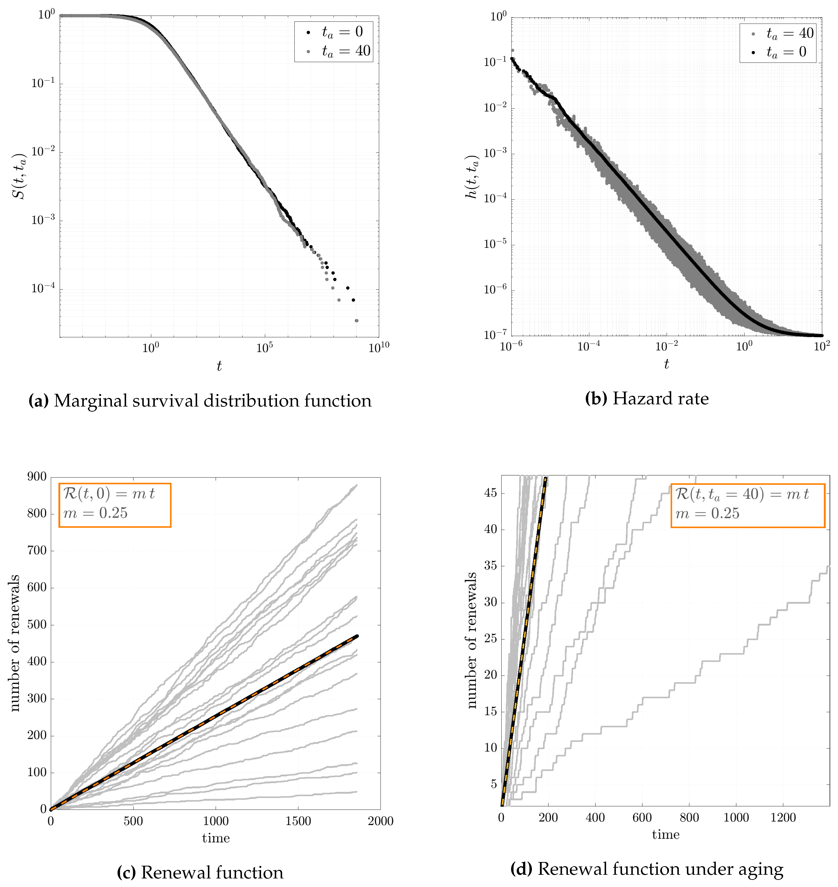
The exponential distribution serves as a mathematical framework for events characterized by a consistent failure rate, making it a staple in reliability analysis. It derives from a Poisson point process where events occur with a constant intensity. Practitioners often rely on this distribution under the assumption that the failure rate remains constant or undergoes negligible change, simplifying the computation of reliability metrics. In superstatistics literature, it is about obtaining pareto probability distribution (fat-tail) by mixing exponential distributions using uniform and gamma distributions as weights. We will show that despite the conditional processes exhibit neutral aging, the marginal process, under proper weights, does show effectual aging.
  • At this point we will switch our analysis to an exchangeable sequence, τ which follows an exponential distribution with a rate that is a uniform random variable, i.e., τ i | λ EXP ( λ ) with the rate undergoing to λ U ( 0 , 2 m ) . The marginal density function of the waiting times ψ τ i ( a ) ( t ) is given by the unconditional mixed-type pdf as from eq.(12):
    ψ τ i ( a ) ( t ) = f ( t , t a ) = 0 2 m f ( t , t a | λ ) 1 2 m d λ = 1 e 2 m t ( 2 m t + 1 ) / t 2 = ψ τ i ( t )
    The equation above is valid since the conditional aged probability density function can be written as f ^ ( u , s a | λ ) = λ / s a ( u + λ ) so that the conditional aged pdf is equal to the non-aged one:
    f ( t , t a | λ ) = L u 1 L s a 1 λ s a ( u + λ ) = L u 1 λ ( u + λ ) L s a 1 1 s = = λ e λ t = f ( t , 0 | λ )
    Essentially, in this example case the renewal process is affected by neutral aging. Moreover, the mixed renewal function R ( t ) can be written in terms of the laplace transform as from proposition 4:
    R ^ ( u , t a ) = 0 2 m f ^ ( u , t a | λ ) u ( 1 f ^ ( u , t a | λ ) ) 1 2 m d λ = 1 2 m 0 2 m λ u + λ u u u + λ d λ = m u 2
    so the mean rate of events is:
    R ( t , t a ) = m t ,
    so that the average number of renewals increases linearly with time even in presence of aging since it is independend from the latency period t a .
    Moreover, as regarding the hazard rate, we have:
    h ( t , t a ) = f ( t , t a ) S ( t , t a ) = 1 ( 1 + 2 m t ) e 2 m t 1 e 2 m t 1 t t 1
    so that the hazard rate is a decreasing function, which is different from its conditional hazard counterpart which is constant. Finally, the asymptotic mean residual lifetime is m ( t , t a ) t .
    as expected. In Figure 2 we compare tha analytical results with simulations in the case of m = 0.25 . plot the marginal distribution of τ i which follows a fat-tail distribution function with an asymptotic behavior of ψ τ i ( a ) ( t ) t 2 .
  • As a more general example, let assume again τ i | λ EXP ( λ ) but now the exponential rate follows a gamma distribution i.e., λ GA ( α , β ) , where α is the shape factor and β is the scale factor. So, in this case, the marginal density function of the waiting times ψ τ i ( a ) ( t ) is given by the unconditional mixed-type pdf:
    ψ τ i ( a ) ( t ) = f ( t , t a ) = 0 f ( t , t a | λ ) β Γ ( α ) λ α 1 e β λ d λ = α β α ( β + t ) α + 1
    which is is a Pareto Lomax density function. So, even in this case, the process shows a neutral aging since there is no dependence on the latency period t a . In addition, it is straightforward to see that the unconditional hazard function is:
    h ( t , t a ) = α β α ( β + t ) α + 1 ( β + t ) α β α = α β + t t 1
    Consequently, the cumulative hazard rate is H ( t , t a ) = α ln t . Similarly, one can find that the mean residual lifetime asymptotic behavior is m ( t , t a ) t . Finally, the mixed renewal function can be written as:
    R ^ ( u , t a ) = β u 2 Γ ( α ) 0 λ α e β λ d λ = m u 2 = β u 2 Γ ( α ) β α 1 Γ ( α + 1 )
    so the average number of renewals is:
    R ( t , t a ) = α β α t ,
    which increases linearly with time even in presence of aging as in the previous example.
    Essentially, all the survival analysis is quite similar to the one in previous example.

4.1.2. Mixture of Generalized Exponentials

The purpose of using the following class of mixture, is to show how to obtain a exponential distributions affected by effective aging, rather than neutral, if the process is a proper mixture of events. Let us take an example, where we see the effective aging, and consider a τ i | θ GA ( α , θ ) with constant shape parameter α and a random scale parameter θ . The Gamma distribution finds frequent reliability studies in characterizing phenomena where consecutive events or perturbations contribute to eventual system failure, as well as in modeling renewal processes. The shape parameter, may be interpreted as the number of events till failure meanwhile the scale parameter represents the rate or frequency of events.
In this case, the generic marginal density function of the waiting times is given by the unconditional mixed-type probability density:
f ^ ( u , s a | θ ) = 1 ( 1 + θ s a ) α 1 ( 1 + θ u ) α ( u s a ) ( 1 1 ( 1 + θ s a ) α )
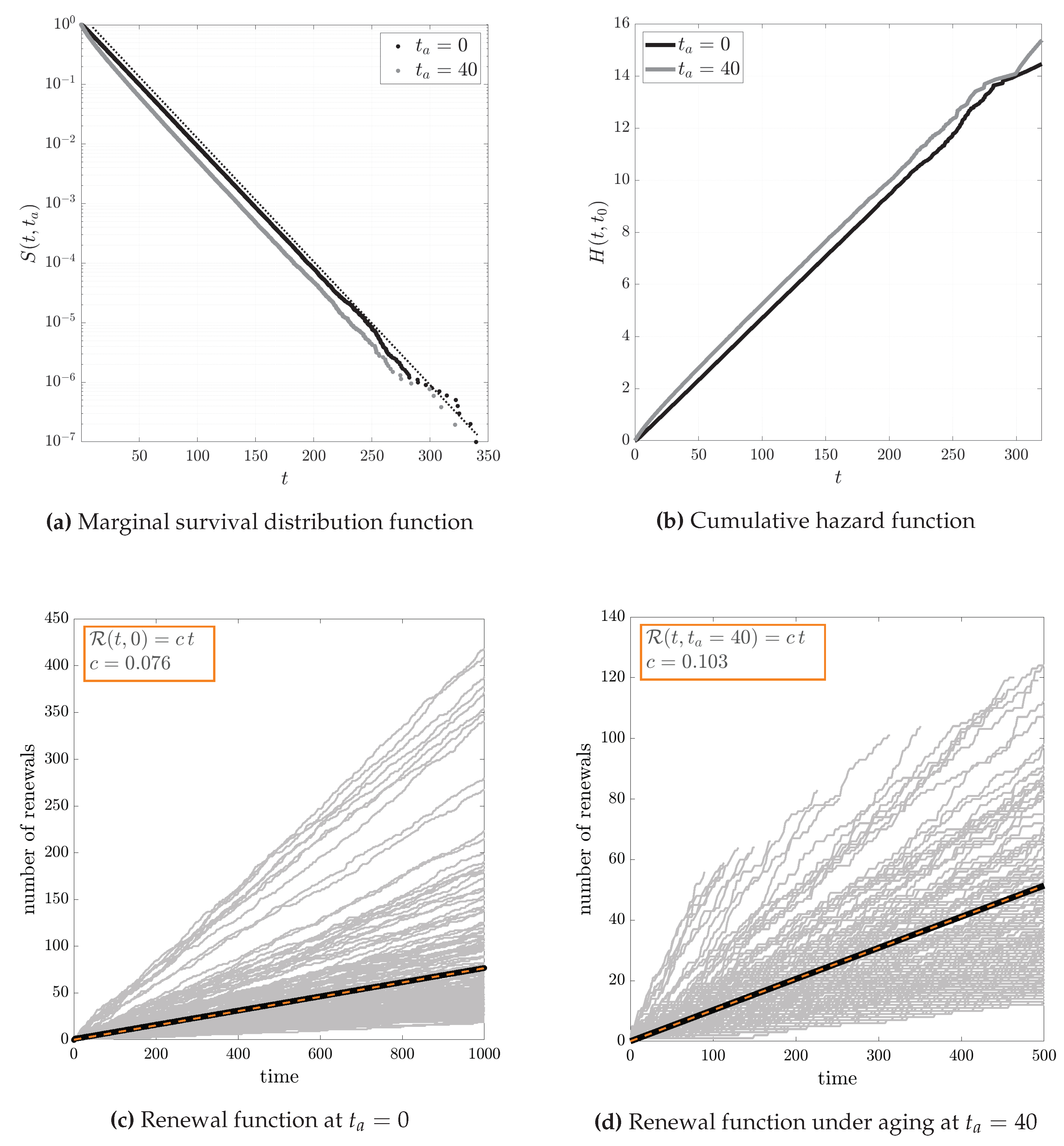
In particular, a gamma distributed random variable with α = 2 and θ uniformly distributed θ U ( m , M ) , marginally yields an exponential distribution which is affect by aging, and the probability density, as derived in Appendix A.1, has the following asymptotic function:
f ( t , t a ) = 1 2 ( M m ) e t M m 1 + e 2 t a M m
which clearly shows the presence of effective aging on the mixed renewal process since the aged marginal pdf is f ( t , t a ) f ( t ) . In conclusion, in this example, despite the unconditional pdf is of the exponential type, the renewal process exhibits effective aging. Subsequently, the cumulative hazard function is:
H ( t , t a ) = ln S ( t , t a ) = 1 M m t log 1 2 + e 2 t a M m t 2 + 4 t a ,
which is asymptotically linear respect to t for large times.
Finally, the mixed renewal function R ( t ) has the following asymptotic behavior:
R ( t , t a ) = ln M ln m 2 ( M n ) + 1 4 M m t a t for t a 0 +
4 ( ln M ln m ) 3 ( M m ) t for t a
as derived in Appendix A. Let us notice that in the asymptotic behavior of the brand new renewal function, the average number of renewals increases linearly with a constant of c = ln M ln m 2 ( M n ) .
We highlight as the numerical simulations as in Figure 3 fully confirm the analytical prediction for renewal aging in the survival analysis: the marginal distribution function from eq.(25), the cumulative hazard rate in eq.(26) and the renewal function eq.(27) have the behavior without and with aging as predicted by the analytical calculations.

4.1.3. Mixture of Heavy-Tail Distributions

In this example, we discuss μ - mixed renewal processes with Mittag-Leffler inter-arrival time distribution. The Mittag-Leffler waiting time distribution is studied by many authors and has considerable applications [55,56] since it can characterize both heavy and fat tails, meaning that there is higher probability of observing extreme values compared to some other distributions like the exponential. In mathematics, the Mittag-Leffler functions play an important role in fractional calculus and stochastic models [57,58,59]. Let us assume that τ i | θ ML ( α , λ ) where the Mittag-Leffler probability distribution is defined in terms of its survival function for λ > 0 and 0 < α 1 as:
S ( t | ( α , λ ) ) = E α ( ( λ t ) α ) n = 0 ( 1 ) n Γ ( 1 + n α ) ( λ t ) n α = 1 ( λ t ) α Γ ( 1 + α ) e ( λ t ) α Γ ( 1 + α ) as t 0 + 1 Γ ( 1 α ) ( λ t ) α as t +
showing two types of heavy-tail behaviors i.e., the stretched exponential (subexponential-type) and the inverse power-law (Pareto-type) distributions. The ML distribution can be easily written in the Laplace space as S ^ = ( u + λ α u α 1 ) 1 so that the pdf is f ^ = ( 1 + ( u / λ ) α ) 1 . Consequently, in double Laplace space, the conditional Mittag-Leffler probability density function under aging with latecy t a can be written as:
f ^ ( u , s a | ( α , λ ) ) = 1 ( s a / λ ) α + 1 1 ( u / λ ) α + 1 ( u s a ) ( 1 1 ( s a / λ ) α + 1 ) = ( u / s a ) α 1 u / s a 1 f ^ o ( u , s a | ( α , λ ) )
where we have indicated the original (brand new) conditional pdf at t a = 0 ad:
f ^ o ( u , s a | ( α , λ ) ) : = lim s a + f ^ ( u , s a | ( α , λ ) ) = 1 s a ( 1 + ( u / λ ) α )
Consequently, the unconditional pdf is given in general by:
f ^ ( u , s a ) = Θ ( u / s a ) α 1 u / s a 1 f ^ o ( u , s a | θ ) d Π ( θ )
where θ = ( α , λ ) .
In particular, let us take α constant, and the scale parameter λ a uniform random variable with λ U ( 0 , T ) . Consequently, the aged marginal probability density, as derived in Appendix A , as the following asymptotic expression:
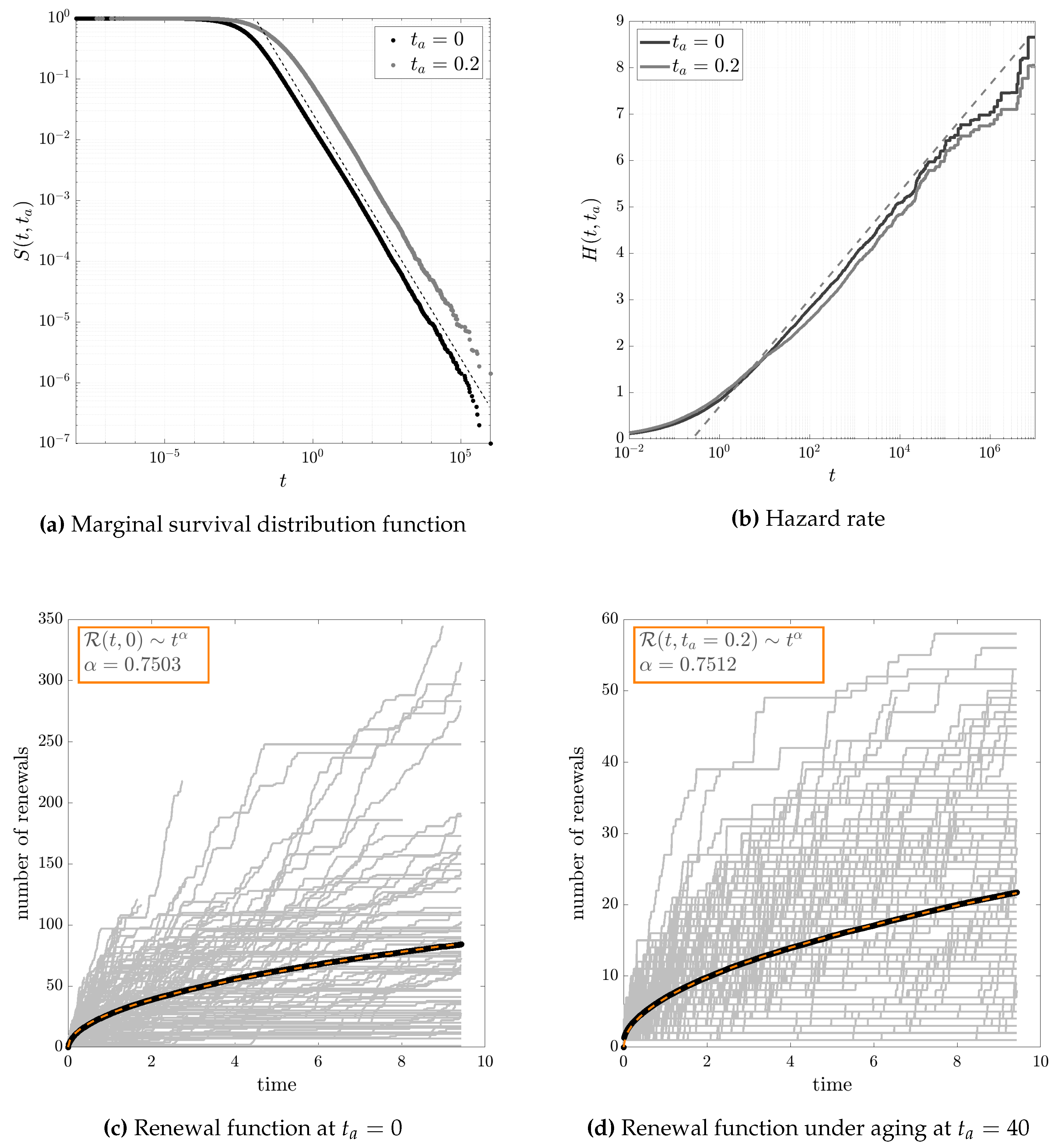
f ( t , t a ) = Λ α ( α 1 ) Γ ( α ) 1 + c α t a α t α t ( 1 + α )
where c α = Γ ( α ) Γ ( 1 + α ) Γ ( 2 α ) if α 1 / 2 and c 1 / 2 = 1 .
Subsequently, the cumulative hazard rate is:
H ( t , t a ) = ln 1 t α + c α 2 t a α t 2 α + ln Λ α α ( α 1 ) Γ ( α )
which for times much larger than the latency period, reads as H ( t , t a ) = t α ln t .
Finally, as derived in, the mixed renewal function reads:
R ( t , t a ) = ( Λ t ) α Γ ( 1 + α ) for t a = 0
( Λ t ) α Γ ( 1 + α ) + Q ( t α ) for t a 0 , t
where Q ( t α ) is a function of t α but asymptotically independent on time. Thus, for α < 1 the renewal function turns out super-linear for small t and sub-linear for large t.

4.2. Case Study: High Frequency Exchange Rates

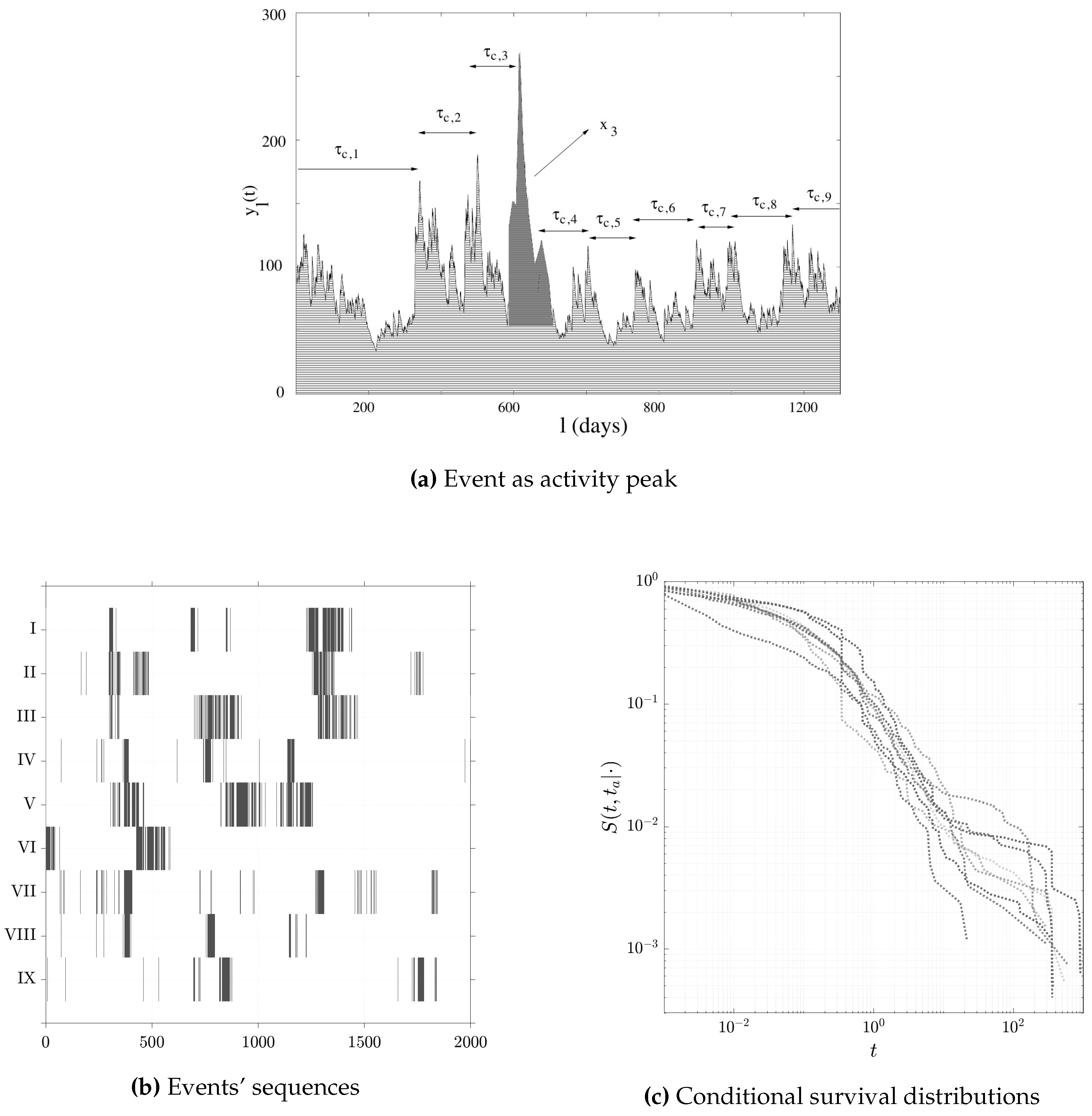
Here, we analyse the times between successive events of the exchange rate transactions. In particular, financial time series exhibit a pronounced non-uniform temporal pattern, particularly concerning aspects like volatility and activity defined as the number of transactions per unit of time [60,61,62]. When examining the return variance within a given time frame, one can discern periods of relatively constant and predictable behavior interspersed with intervals characterized by significant variations in price (or exchange rate). Similarly, fluctuations exist in the frequency of transactions, with some days witnessing sparse trading and others marked by a considerably higher volume of trades. This substantial variability in both volatility and activity is commonly denoted as volatility clustering or intermittency in volatility and activity which have a proportional relationship as discussed in literature of financial volatility modeling [63,64,65,66]. As an example of real world financial sequences, we will make use of currency pairs with tick-by-tick historical rates retrieved from [67]. In particular, we use top-of-book tick-by-tick market data, with fractional pip spreads in millisecond detail. So they represent ultra high frequency data for exchange rates markets. We have used exchange rates for 9 different currency pairs in Table 1 whose transactions occurred in the month of November 2023 at the level of tick-by-tick data for a total of about 10 7 ticks with a time resolutions of milliseconds.
Moreover, each tick represents a trade (transaction) and we call it a marker of the time series. Time intervals between two consecutive markers are not independent because of the presence of peaks (or clusters) in the mean activity followed by periods of relative calm. In order to detect meaningful insights we define as events the peaks of activity (i.e., the event of volatility clustering) which are separated by periods with a low number of transactions. We use a peak detection algorithm in order to define the events of intense activity out of the tick markers ( Threshold has been used as minimum height difference between a peak and its neighbors, so to detect abrupt changes.). In Figure 5 we see a schematic representation where the intensity, for example, x3 of the third peak corresponds to the total number of transactions attributed to this peak. In Figure 5 the arrivals of events are plotted for all the nine exchange rate time series. Finally, in Figure 5 we show their conditional distributions.
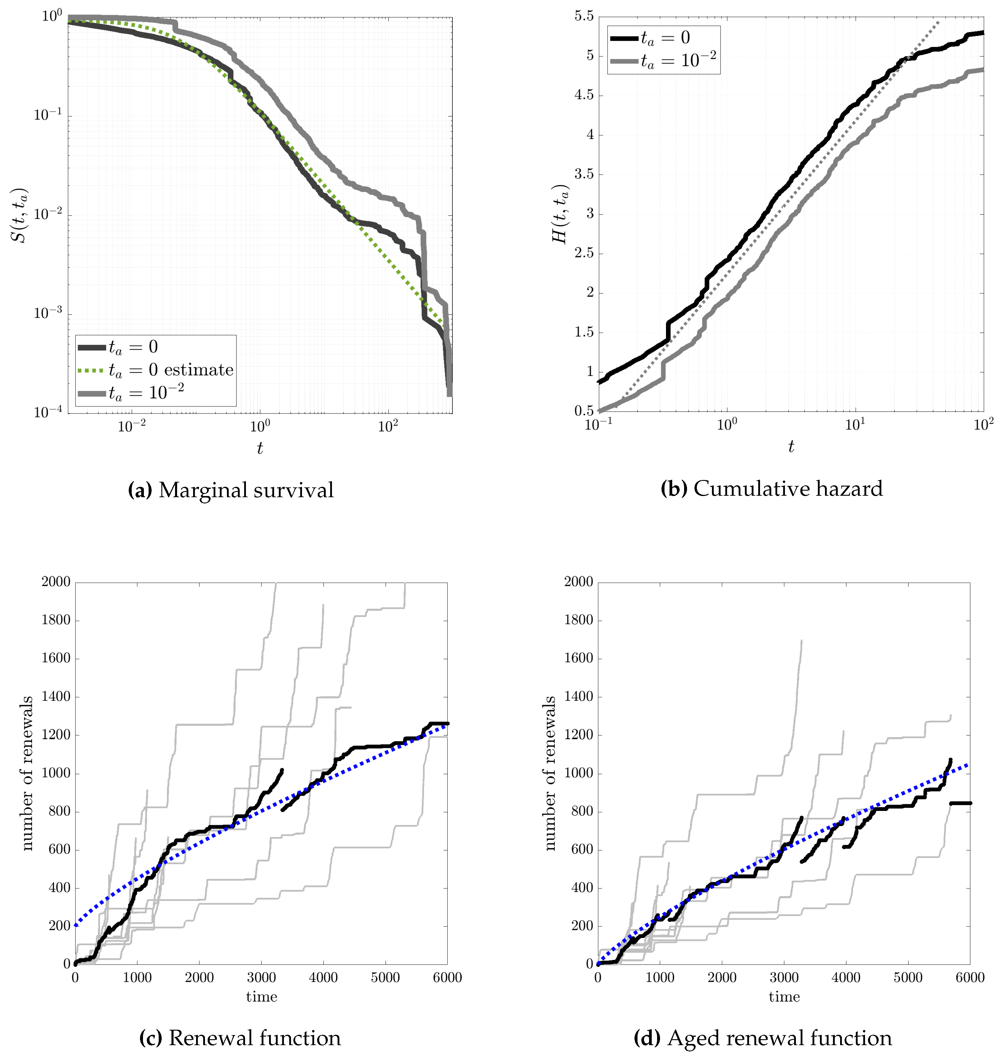
Despite the discussion about financial modeling is out of the purpose in this study, the analysis presented herein can offer valuable perspectives for empirical interpretations in the examination of financial market dynamics of price fluctuations in high-frequency trading [29,68,69]. The survival analysis in Figure 6 illustrates that the empirical process responsible for generating exchange rate events is compatible with a Mittag-Leffler function as a prior distribution. As possible implications we observe, in Figure 6, that the time intervals between peaks, denoted as τ c , follow a probability density function ψ ( τ c ) that asymptotically behaves as ψ ( τ c ) 1 / τ c ν , with ν 1.75 . Furthermore, we identify the occurrence of unconditional negative aging, given that S ( τ c ( a ) ) > S ( τ c ) , implying that the aged variable τ c ( a ) is greater than the original τ c in stochastic ordering. The event-time distribution is thus characterized as new worse than observed, signifying that a latency in the event detection process creates an illusion of the system performing better than its actual behavior. In other words, the system exhibits a reduced probability of events occurring immediately after activation (latency period). Similarly, in Figure 6 comparing the two cumulative hazard rate functions, one can notice that, since the aged cumulative hazard rate function is stochastically smaller than the brand new one, it implies that the aged process has a lower cumulative risk of volatility events. Finally the analysis of the renewal function in Figure 6 indicates that the expected number of arrivals is nonlinear, a behavior maintained even after aging, as shown in Figure 6.

5. Concluding Remarks

In our research within the domain of reliability theory, we have introduced the idea of statistical aging as latency, specifically in the framework of mixed renewal processes where the intervals between events are considered exchangeable. This approach provides a more accurate representation of the interdependence among failure events that occur at unpredictable intervals, while preserving manageability. Simultaneously, it acknowledges some level of dependence among events. Furthermore, it is important to note that the event rate of a system can display fluctuations due to a variety of aging and latency factors. These can include environmental conditions, operational stresses, or delays in detection. The findings of this paper consist in a set of new propositions which asses how latency aging affects the survival analysis of mixed renewal processes. Survival and aging analysis involves analyzing data on the time until an event of interest occurs and is particularly relevant in finance due to the importance of modelling risk and uncertainty [70,71]. From that perspective, we have provided evidence that exchange rates can be affected by a “new worse than observed” event distribution, which implies that detection latency can make the system appear more efficient than it truly is, with a decreased likelihood of immediate post-activation events. Concurrently, an aged process exhibits a diminished cumulative risk of volatility events.
In a subjective probability perspective of complex systems, the notion of mixed renewal processes is related to the concept of superstatistics, which indicates a superposition of several statistics on different scales [43,72]. A superstatistical interpretation of renewal processes has been applied in various fields, including financial markets, traffic delays, air pollution dynamics and hydrodynamic turbulence [73,74,75,76]. A future research direction will be the development of a event-sequence technique which may detect the presence of memory between the events through the effect of renewal aging. Such problem is of great interest in reliability assessment research [77,78] with an assumption that events are exchangeable rather than independent and identically distributed which is a common hypothesis that may not always be valid, especially in cases where repairs fail to fully restore the system. Renewal aging can be exploited as a crucial property to determine whether a pattern of events is compatible with a renewal process in the classical sense of being i.i.d. rather than in the exchangeability sense. In terms of policy implications, financial institutions and investors can make informed decisions by considering the changing dynamics of market behaviour influenced by fixed latency periods and their associated aging patterns.

Author Contributions

Conceptualization, F.V., D.L.; methodology, F.V., D.L.; software, F.V.; validation, F.V., D.L.; formal analysis, F.V., D.L.; investigation, F.V., D.L.; resources, F.V., D.L.; data curation, F.V.; writing—original draft preparation, F.V., D.L. ; writing—review and editing, F.V., D.L.; visualization, F.V. ; supervision, F.V., D.L.; project administration, F.V., D.L.. All authors have read and agreed to the published version of the manuscript.

Funding

D.L. has received a support for the work funded by ….

Data Availability Statement

The data presented in this study are available in truefx website at https://www.truefx.com/truefx-historical-downloads.

Acknowledgments

F.V. wants to acknowledge to be a member of GNAMPA-INdAM.

Conflicts of Interest

The authors declare no conflicts of interest.

Abbreviations

The following abbreviations are used in this manuscript:
CDF Cumulative Distribution Function
eCDF empirical Cumulative Distribution Function
pdf probability density function
i.i.d. independent identically distributed
DP Dirichlet Process
EXP Exponential
GA Gamma
ML Mittag-Leffler

Appendix A. Mixture Models Derivations

Appendix A.1. Derivation of eq.(uid48):

We can write the double Laplace transform of the aged conditional pdf as:
f ^ ( u , s a | θ ) = 1 + θ u θ s a + 2 f ^ o ( u , s a | θ )
where
f ^ o ( u , s a | θ ) : = lim s a + f ^ ( u , s a | θ ) = 1 s a ( 1 + θ u ) 2
is the original, brand new, conditional pdf without any latency effect on the mixed renewal process. Then, the single space Laplace transform of the conditional pdf is:
f ^ ( u , t a | θ ) = L s a 1 { f ^ ( u , s a | θ ) } = 1 + θ u 2 ( 1 e 2 t a / θ ) f ^ ( u , 0 | θ )
Consequently, moving back to time variable, the asymptotic expression of the aged unconditional probability density is:
f ( t , t a ) = L u 1 m M f ^ ( u , t a | θ ) 1 M m d θ t 1 2 ( M m ) e t M m 1 + e 2 t a M m

Appendix Derivation of eq.(uid50):

The mixed renewal function R ( t ) can be written in terms of the laplace transform as from proposition 4:
R ( u , t a ) = 1 M m m M 1 + θ u 2 1 e 2 t a / θ θ u 2 θ u + 2 1 2 ( 1 e 2 t a / θ ) d θ u 0 1 M m m M 1 θ u 2 2 1 2 ( 1 e 2 t a / θ ) + 1 e 2 t a / θ u 2 1 2 ( 1 e 2 t a / θ ) d θ
which, for large times, can be directly expressed as:
R ( t , t a ) t t M m m M 1 θ 3 2 + 1 2 e 2 t a / θ d θ + 1 M m m M 1 e 2 t a / θ 3 2 + 1 2 e 2 t a / θ d θ
t ln M ln m 2 ( M n ) + 1 4 M m t a t + ln M ln m M m t a for t a m
4 ( ln M ln m ) 3 ( M m ) t for t a M

Appendix Derivation of eq.(uid57):

f ^ ( u , s a ) = 0 Λ f ^ ( u , s a | λ ) π ( λ ) d λ = ( u / s a ) α 1 u / s a 1 0 Λ 1 s a ( 1 + ( u / λ ) α ) π ( λ ) d λ = ( u / s a ) α 1 u / s a 1 f ^ o ( u , s a )
where f ^ o ( u , s a ) represent the brand new density. Therefore, according to the definition 4, the process always exhibits an effective aging, since f ( t , t a ) f ( t ) , t a > 0 . In particular, we can calculate the brand-new mixture type probability density trough the following marginal function:
f ^ o ( u , s a ) = 0 Λ f ^ o ( u , s a | λ ) 1 Λ d λ = 1 Λ s a 0 Λ λ α u α + λ α d λ = 1 s a F 1 2 1 , 1 α , 1 1 α , u Λ α 1 s a u 0 1 s a 2 ( u / Λ ) α for α = 1 / 2 1 s a n = 1 ( 1 ) n + 1 ( u / Λ ) n α n α 1 for α 1 / 2
where F 1 2 is first hypergeometric function. So the the asymptotic aged marginal pdf in Laplace space in eq.(A4) as:
f ^ ( u , s a ) u 0 1 s a j = 1 ( u / s a ) j 1 ( u / s a ) a + j 1 f ^ o ( u , s a )
At slowest order s a f ^ ( u , s a ) ( 1 ( u / s a ) α ) ( u / Λ ) α / ( α 1 ) , so, one can write the asymptotic behavior of the unconditional aged pdf in time variable in the regime of large times ( t ) as:
f ( t , 0 ) = L u 1 L s a 1 { f ^ o ( u , s a ) } t Λ α ( α 1 ) Γ ( α ) t ( 1 + α )
f ( t , t a ) = L u 1 L s a 1 { f ^ ( u , s a ) } t 1 + c α t a α t α f ( t , 0 )
where c α = Γ ( α ) Γ ( 1 + α ) Γ ( 2 α ) if α 1 / 2 and c 1 / 2 = 1 .

Appendix Derivation of eq.(uid58):

Let us now focus on the mixed renewal function R ( t ) . It can be written in terms of the laplace transform as from proposition 4 as:
R ^ ( u , t a ) = 0 Λ f ^ ( u , t a | λ ) u ( 1 f ^ ( u , t a | λ ) ) 1 Λ d λ
where:
f ^ ( u , t a | λ ) = L s a 1 ( u / s a ) α 1 ( u / s a 1 ) 1 s a 1 1 + ( u / λ ) α u 0 L s a 1 1 ( u / s a ) α s a 1 1 + ( u / λ ) α f ^ 1 ( u , t a | λ ) Γ ( 1 + α ) ( 1 + ( u / λ ) α ) Γ ( 1 + α ) ( u t a ) α
so the renewal function can be written for large times u 0 as:
R ^ ( u , t a ) = 0 Λ 1 u ( f ^ 1 ( u , t a | λ ) 1 ) 1 Λ d λ = Γ ( 1 + α ) ( t a u ) α Λ u 1 + α 0 Λ λ α Γ ( 1 + α ) + ( t a λ ) α d λ = Γ ( 1 + α ) Λ u 1 + α t a α u Λ Λ 1 + α ( 1 + α ) Γ ( 1 + α ) F 1 2 1 , 1 + 1 α ; 2 + 1 α ; ( t a Λ ) α Γ ( 1 + α )

References

  1. Feller, W. An introduction to probability theory and its applications; Vol. 1, John Wiley & Sons, 1968.
  2. Feller, W. An introduction to probability theory and its applications; Vol. 2, John Wiley & Sons, 1991.
  3. Cox, D.R. Renewal theory; Vol. 1, Methuen London, 1967.
  4. Barlow, R.E.; Proschan, F. Statistical theory of reliability and life testing: Probability models; Vol. 1, Holt, Rinehart and Winston New York, 1975.
  5. Lio, Y.; Chen, D.G.; Ng, H.T.; Tsai, T.R. Bayesian Inference and Computation in Reliability and Survival Analysis; Springer, 2022.
  6. Mitov, K. Renewal processes; Springer: Cham, 2014. [Google Scholar]
  7. Cha, J.H.; Finkelstein, M. ; others. Point processes for reliability analysis, 2018. [Google Scholar]
  8. De Finetti, B. Funzione caratteristica di un fenomeno aleatorio. Atti del Congresso Internazionale dei Matematici: Bologna del 3 al 10 de settembre di 1928, 1929, pp. 179–190. [Google Scholar]
  9. De Finetti, B. La prévision: Ses lois logiques, ses sources subjectives. Annales de l’institut Henri Poincaré 1937, 7, 1–68. [Google Scholar]
  10. Aldous, D.J. Exchangeability and related topics. In École d’Été de Probabilités de Saint-Flour XIII—1983; Springer, 1985; pp. 1–198.
  11. Bernardo, J.M.; Smith, A.F. Bayesian theory; Vol. 405, John Wiley & Sons, 2009.
  12. Coen, A.; Gutiérrez, L.; Mena, R.H. Modelling failures times with dependent renewal type models via exchangeability. Statistics 2019, 53, 1112–1130. [Google Scholar] [CrossRef]
  13. Huang, W.J. On the characterization of point processes with the exchangeable and Markov properties. Sankhyā: The Indian Journal of Statistics, Series A.
  14. Lyberopoulos, D.P.; Macheras, N.D. Some characterizations of mixed renewal processes. Mathematica Slovaca 2022, 72, 197–216. [Google Scholar] [CrossRef]
  15. Metzler, R.; Jeon, J.H.; Cherstvy, A.G.; Barkai, E. Anomalous diffusion models and their properties: Non-stationarity, non-ergodicity, and ageing at the centenary of single particle tracking. Physical Chemistry Chemical Physics 2014, 16, 24128–24164. [Google Scholar] [CrossRef] [PubMed]
  16. Bianco, S.; Grigolini, P.; Paradisi, P. Fluorescence intermittency in blinking quantum dots: Renewal or slow modulation? The Journal of chemical physics 2005, 123. [Google Scholar] [CrossRef] [PubMed]
  17. Laloux, L.; Le Doussal, P. Aging and diffusion in low dimensional environments. Physical Review E 1998, 57, 6296. [Google Scholar] [CrossRef]
  18. Godreche, C.; Luck, J. Statistics of the occupation time of renewal processes. Journal of Statistical Physics 2001, 104, 489–524. [Google Scholar] [CrossRef]
  19. Monthus, C.; Bouchaud, J.P. Models of traps and glass phenomenology. Journal of Physics A: Mathematical and General 1996, 29, 3847. [Google Scholar] [CrossRef]
  20. Parisi, G. Short-time aging in binary glasses. Journal of Physics A: Mathematical and General 1997, 30, L765. [Google Scholar] [CrossRef]
  21. Baity-Jesi, M.; Calore, E.; Cruz, A.; Fernandez, L.; Gil-Narvion, J.; Gonzalez-Adalid Pemartin, I.; Gordillo-Guerrero, A.; Iñiguez, D.; Maiorano, A.; Marinari, E. ; others. Memory and rejuvenation effects in spin glasses are governed by more than one length scale. Nature Physics.
  22. Böhmer, T.; Gabriel, J.P.; Costigliola, L.; Kociok, J.N.; Hecksher, T.; Dyre, J.C.; Blochowicz, T. Time reversibility during the ageing of materials. Nature Physics.
  23. Barkai, E. Aging in subdiffusion generated by a deterministic dynamical system. Physical review letters 2003, 90, 104101. [Google Scholar] [CrossRef] [PubMed]
  24. Akimoto, T.; Barkai, E. Aging generates regular motions in weakly chaotic systems. Physical Review E 2013, 87, 032915. [Google Scholar] [CrossRef]
  25. Gupta, A.K.; Zeng, W.B.; Wu, Y. Probability and statistical models: Foundations for problems in reliability and financial mathematics; Springer Science & Business Media, 2010.
  26. Hens, T.; Schenk-Hoppé, K.R. Handbook of financial markets: Dynamics and evolution; Elsevier, 2009.
  27. Barbiero, A.; Hitaj, A. Discrete half-logistic distributions with applications in reliability and risk analysis. Annals of Operations Research.
  28. Bianco, S.; Grigolini, P. Aging in financial market. Chaos, Solitons & Fractals 2007, 34, 41–50. [Google Scholar]
  29. Fama, E.F. The behavior of stock-market prices. The journal of Business 1965, 38, 34–105. [Google Scholar] [CrossRef]
  30. Cherstvy, A.G.; Vinod, D.; Aghion, E.; Chechkin, A.V.; Metzler, R. Time averaging, ageing and delay analysis of financial time series. New journal of physics 2017, 19, 063045. [Google Scholar] [CrossRef]
  31. Niepert, M.; Domingos, P. Exchangeable variable models. International Conference on Machine Learning, 2014, pp. 271–279.
  32. Poirier, D.J. 40 Exchangeability, Representation Theorems, and Subjectivity. In The Oxford Handbook of Bayesian Econometrics; Oxford University Press, 2011; [https://academic.oup.com/book/0/chapter/334662922/chapter-ag-pdf/44445457/book_38595_section_334662922.ag.pdf]. [CrossRef]
  33. Hewitt, E.; Savage, L.J. Symmetric measures on Cartesian products. Transactions of the American Mathematical Society 1955, 80, 470–501. [Google Scholar] [CrossRef]
  34. Diaconis, P.; Freedman, D. Finite exchangeable sequences. The Annals of Probability.
  35. Kerns, G.J.; Székely, G.J. Definetti’s theorem for abstract finite exchangeable sequences. Journal of Theoretical Probability 2006, 19, 589–608. [Google Scholar] [CrossRef]
  36. Kallenberg, O. Probabilistic Symmetries and Invariance Principles; Springer New York: New York, NY, 2005. [Google Scholar]
  37. O’Neill, B. Exchangeability, correlation, and Bayes’ effect. International statistical review 2009, 77, 241–250. [Google Scholar] [CrossRef]
  38. Barber, R.F.; Candes, E.J.; Ramdas, A.; Tibshirani, R.J. De Finetti’s Theorem and Related Results for Infinite Weighted Exchangeable Sequences. arXiv preprint arXiv:2304.03927, arXiv:2304.03927 2023.
  39. Zabell, S.L. Predicting the unpredictable. Synthese 1992, 90, 205–232. [Google Scholar] [CrossRef]
  40. Bernardo, J.M. Bayesian statistics. Probability and Statistics, R. Viertl, Ed 1994, 2, 345–407. [Google Scholar]
  41. Bernardo, J.M. The concept of exchangeability and its applications. Far East Journal of Mathematical Sciences 1996, 4, 111–122. [Google Scholar]
  42. Brokmann, X.; Hermier, J.P.; Messin, G.; Desbiolles, P.; Bouchaud, J.P.; Dahan, M. Statistical aging and nonergodicity in the fluorescence of single nanocrystals. Physical review letters 2003, 90, 120601. [Google Scholar] [CrossRef] [PubMed]
  43. Allegrini, P.; Barbi, F.; Grigolini, P.; Paradisi, P. Renewal, modulation, and superstatistics in times series. Physical Review E 2006, 73, 046136. [Google Scholar] [CrossRef] [PubMed]
  44. Paradisi, P.; Grigolini, P.; Bianco, S.; Akin, O.C. Renewal aging in non-homogeneous poisson processes with periodic rate modulation. International Journal of Bifurcation and Chaos 2008, 18, 2681–2691. [Google Scholar] [CrossRef]
  45. Aquino, G.; Bologna, M.; Grigolini, P.; West, B.J. Aging and rejuvenation with fractional derivatives. Physical Review E 2004, 70, 036105. [Google Scholar] [CrossRef] [PubMed]
  46. Allegrini, P.; Aquino, G.; Grigolini, P.; Palatella, L.; Rosa, A.; West, B.J. Correlation function and generalized master equation of arbitrary age. Physical Review E 2005, 71, 066109. [Google Scholar] [CrossRef] [PubMed]
  47. Bernstein, D.L. The double Laplace integral. Duke Mathematical Journal 1941, 8(3), 460–496. [Google Scholar] [CrossRef]
  48. Debnath, L.; Bhatta, D. Integral transforms and their applications; Chapman and Hall/CRC, 2016; chapter 4.
  49. Aquino, G.; Palatella, L.; Grigolini, P. Absorption and emission in the non-poisson case: The theoretical challenge posed by renewal aging. Brazilian journal of physics 2005, 35, 418–424. [Google Scholar] [CrossRef]
  50. Spizzichino, F. Subjective probability models for lifetimes; CRC Press, 2001.
  51. Lai, C.D.; Xie, M. Stochastic ageing and dependence for reliability; Springer Science & Business Media, 2006.
  52. Nappo, G.; Spizzichino, F. Relations between ageing and dependence for exchangeable lifetimes with an extension for the IFRA/DFRA property. Dependence Modeling 2020, 8, 1–33. [Google Scholar] [CrossRef]
  53. McCall, J.J. ; others. An introduction to exchangeability and its economic applications, 1988. [Google Scholar]
  54. Faragó, A. Decomposition of Random Sequences into Mixtures of Simpler Ones and Its Application in Network Analysis. Algorithms 2021, 14, 336. [Google Scholar] [CrossRef]
  55. Mainardi, F.; Gorenflo, R.; Vivoli, A. Renewal Processes of Mittag-Leffler and Wright Type. Fractional Calculus and Applied Analysis 2005, 8, 07–38. [Google Scholar]
  56. Mainardi, F.; Raberto, M.; Gorenflo, R.; Scalas, E. Fractional calculus and continuous-time finance II: The waiting-time distribution. Physica A: Statistical Mechanics and its Applications 2000, 287, 468–481. [Google Scholar] [CrossRef]
  57. Pramukkul, P.; Svenkeson, A.; Grigolini, P.; Bologna, M.; West, B.; others. Complexity and the fractional calculus. Advances in Mathematical Physics 2013, 2013. [Google Scholar] [CrossRef]
  58. Apelblat, A. Differentiation of the Mittag-Leffler functions with respect to parameters in the Laplace transform approach. Mathematics 2020, 8, 657. [Google Scholar] [CrossRef]
  59. Gorenflo, R.; Kilbas, A.A.; Mainardi, F.; Rogosin, S.V. ; others. Mittag-Leffler functions, related topics and applications, 2020. [Google Scholar]
  60. Scalas, E.; Gorenflo, R.; Mainardi, F. Fractional calculus and continuous-time finance. Physica A: Statistical Mechanics and its Applications 2000, 284, 376–384. [Google Scholar] [CrossRef]
  61. Gençay, R.; Dacorogna, M.; Muller, U.A.; Pictet, O.; Olsen, R. An introduction to high-frequency finance; Elsevier, 2001.
  62. Palatella, L.; Perelló, J.; Montero, M.; Masoliver, J. Activity autocorrelation in financial markets: A comparative study between several models. The European Physical Journal B-Condensed Matter and Complex Systems 2004, 38, 671–677. [Google Scholar] [CrossRef]
  63. Taylor, S.J. Modeling stochastic volatility: A review and comparative study. Mathematical finance 1994, 4, 183–204. [Google Scholar] [CrossRef]
  64. Pederzoli, C. Stochastic volatility and GARCH: A comparison based on UK stock data. European Journal of Finance 2006, 12, 41–59. [Google Scholar] [CrossRef]
  65. Fouque, J.P.; Papanicolaou, G.; Sircar, K.R. Derivatives in financial markets with stochastic volatility; Cambridge University Press, 2000.
  66. Cont, R. Statistical modeling of high-frequency financial data. IEEE Signal Processing Magazine 2011, 28, 16–25. [Google Scholar] [CrossRef]
  67. Corp., I.D. Corp., I.D. TrueFX Market exchange rate data, 2014. EURUSD exchange rates data retrieved for november 2022 from https://www.truefx.com/truefx-historical-downloads/#93-106-november.
  68. Scalas 7, E.; Gorenflo, R.; Luckock, H.; Mainardi, F.; Mantelli, M.; Raberto, M. Anomalous waiting times in high-frequency financial data. Quantitative Finance 2004, 4, 695–702. [Google Scholar] [CrossRef]
  69. Aldrich, E.M.; Heckenbach, I.; Laughlin, G. The random walk of high frequency trading. arXiv preprint arXiv:1408.3650, arXiv:1408.3650 2014.
  70. Gao, F.; He, X. Survival Analysis: Theory and Application in Finance. In HANDBOOK OF FINANCIAL ECONOMETRICS, MATHEMATICS, STATISTICS, AND MACHINE LEARNING; World Scientific, 2021; pp. 4087–4118.
  71. Gepp, A.; Kumar, K. The role of survival analysis in financial distress prediction. International research journal of finance and economics 2008, 16, 13–34. [Google Scholar]
  72. Beck, C. Superstatistics: Theory and applications. Continuum mechanics and thermodynamics 2004, 16, 293–304. [Google Scholar] [CrossRef]
  73. Uchiyama, Y.; Kadoya, T. Superstatistics with cut-off tails for financial time series. Physica A: Statistical Mechanics and its Applications 2019, 526, 120930. [Google Scholar] [CrossRef]
  74. Schäfer, B.; Heppell, C.M.; Rhys, H.; Beck, C. Fluctuations of water quality time series in rivers follow superstatistics. Iscience 2021, 24. [Google Scholar] [CrossRef] [PubMed]
  75. Katz, Y.A.; Tian, L. Superstatistical fluctuations in time series of leverage returns. Physica A: Statistical Mechanics and its Applications 2014, 405, 326–331. [Google Scholar] [CrossRef]
  76. Beck, C. Recent developments in superstatistics. Brazilian Journal of Physics 2009, 39, 357–363. [Google Scholar] [CrossRef]
  77. Tobias, P.A.; Trindade, D. Applied reliability; CRC Press, 2011.
  78. Wang, P.; Coit, D.W. Repairable systems reliability trend tests and evaluation. Proceedings of the Annual Reliability and Maintainability Symposium. Citeseer, 2005, pp. 416–421.
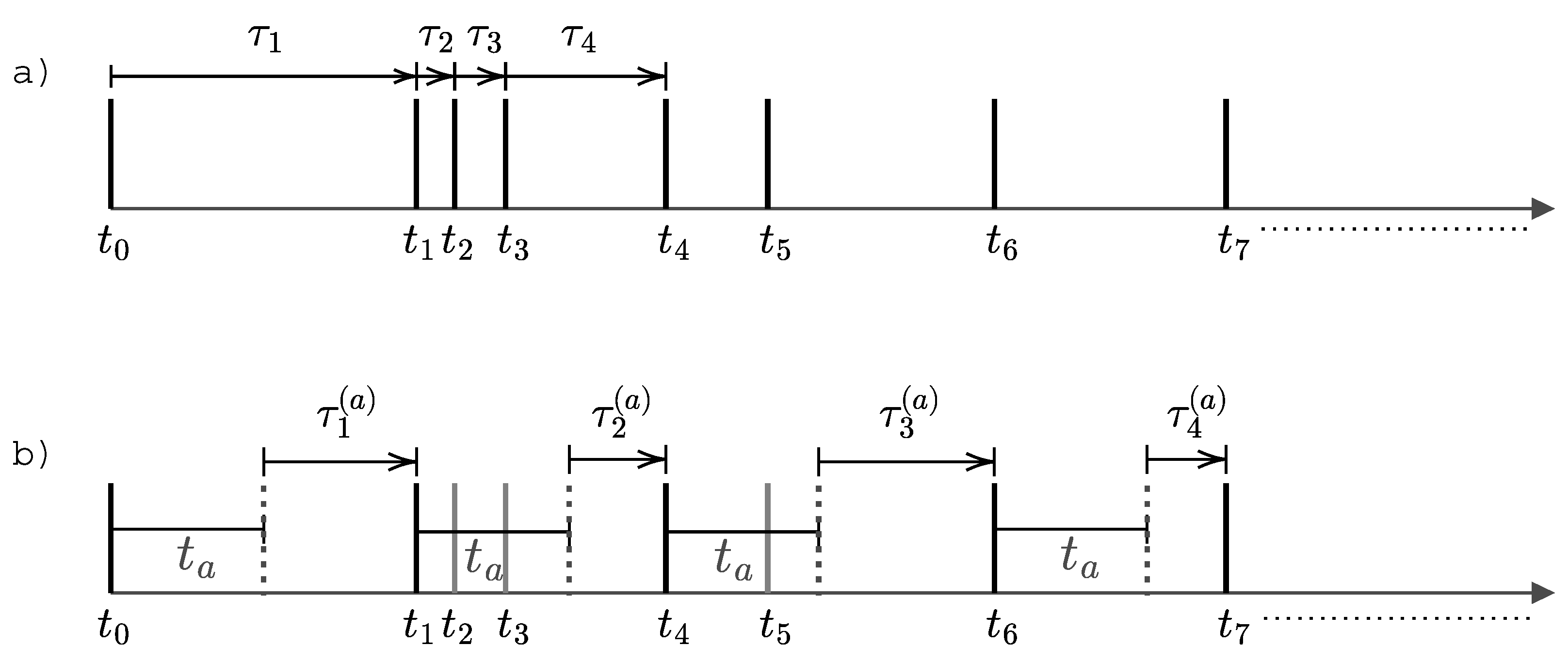
Figure 1. Illustration of an aging experiment for the latency assessment in order to establish the exchangeable renewal nature of the process. In a) we show a sequence of events with inter-event interval times { τ 1 , τ 2 , τ 3 , τ 4 , } . In b) we age the sequence of events using the observation time t a from which the observer is ready to detect the next coming event. So the observer cannot detect any other events before another time t a is passed by, so registering a new aged time intervals τ i ( a ) that are the waiting times for that given latency period of t a > 0 . As consequence, we collect the new (aged) intervals { τ 1 ( a ) , τ 2 ( a ) , τ 3 ( a ) , τ 4 ( a ) , } i.e., the waiting times. Let us notice that, the observation rate in the process could have an impact to the statistical property of the inter-arrival intervals.
Preprints 102386 g001
Figure 2. A μ renewal process where the inter-event time intervals are exponentially distributed conditional to a rate which is a uniform random variable, i.e., τ i | λ EXP ( λ ) with λ U ( 0 , 2 m ) where m = 0.5 . In (a) We see how the marginal survival distribution has a power law tail behavior with f t 2 which does not change after aging so that f ( t , 0 ) = f ( t , t a ) as expected in eq. . In (b) the hazard shows is a decreasing function in t both before and after aging h t 1 as expected. In (c) and (d), finally, we plot the number of renewal events of some conditional iid sequences (in gray), the black bold line represent the renewal function as the average number of events and the orange dashed line the theoretical expected renewal function. The numerical simulations and analytical results are in perfect agreement and the renewal function maintain the same trend event after aging, as predicted.
Preprints 102386 g002
Figure 3. A μ renewal process where the inter-event time intervals are exponentially distributed conditional to a rate which is a uniform random variable, i.e., τ i | λ Ga ( 2 , θ ) with θ U ( m , M ) where m = 1 and M = 21 . In (a) We see how the marginal survival distribution is exponential with estimation f e t / ( M m ) e 0.05 t as expected from eq. (A1). The marginal distribution undergoes to effective aging since f ( t , 0 ) f ( t , t a ) as reperesented by the dotted line. In (b) the cumulative hazard function is linear over t both before and after aging H 0.05 t as predicted by eq.(26), where the shift in the aged rate is also explained. In (c) and (d), finally, we graphically represent the count of renewal events for certain conditionally independent and identically distributed sequences (depicted in gray). The bold black line symbolizes the renewal function, which is the average number of events, while the dashed orange line illustrates the theoretical renewal function. The numerical simulations align perfectly with the analytical outcomes, and as predicted, the renewal function exhibits a shift in trend following the aging process
Preprints 102386 g003
Figure 4. A μ renewal process where the inter-event time intervals are generated conditional to a Mittag-Leffler ML ( 0.75 , λ ) distribution where λ is uniform random variable λ U ( 0 , Λ ) with Λ = 20 . In (a), we see that the marginal survival distribution has a power law tail with coefficient α = 0.5 as expected from eq. (A5). The marginal distribution undergoes to effective aging since S ( t , 0 ) S ( t , t a ) . In (b) the cumulative hazard function is linear over t both before and after aging H 0.5 ln t as predicted by eq.(26), where the shift in the aged rate is also explained. In (c) and (d), finally, we plot through numerical simulations the renewal function is changes after aging. Both cases show in gray some of the trajectories for single sequences of events, in bold black we show the estimated renewal function as average number of events, and in orange dashed line we have the expected renewal function as predicted in eq.(30), with α = 0.75 .
Preprints 102386 g004
Figure 5. XA analysis for EURUSD exchange rates. In (a) there is an schematic example of the definition of inter-event times τ c between two consecutive peaks as activity bursts of large volume of trades y l ( t ) , figure modified from [62]. In (b) we plot arrival sequences of the times between successive peaks for all the nine exchange rate pars. Finally in (c) we show the nine conditional survival distributions of every sequence of temporal events.
Preprints 102386 g005
Figure 6. Survival analysis. In (a) we plot the complementary cumulative distribution function S ( t , t a ) and the estimate of the power law coefficient, showing an asymptotic pareto distribution with exponent α = 0.75 . In (b) we plot the cumulative hazard behavior for both cases of no latency and of a latency of t a = 10 2 . The plot shows that there is only a shift between the two functions and in the central part of the time axis there is a linear trend so that H ( t , t a ) α ln t with α 0.75 . In (c) and in (d) we plot the number of renewal events for all the nine exchange rate sequences (in light gray) and the average number of renewals up to time t (solid black line). Finally, we superimpose (in dotted blue) the expected renewal function under exchangeability assumption for Mittag-Leffler prior so that the asymptotic trend is R t α .
Preprints 102386 g006
Table 1. Exchange rate currency pair names
code Pair Name
I USD/EUR US Dollar/Euro
II USD/AUD US Dollar/Australian Dollar
III USD/GBP US Dollar/British Pound
IV USD/NZD US Dollar/New Zealand Dollar
V USD/CAD US Dollar/Canadian Dollar
VI USD/CHF US Dollar/Swiss Franc
VII USD/JPY US Dollar/Japanese Yen
VIII USD/MXN US Dollar/Mexican Peso
IX USD/ZAR US Dollar/South African Rand
Disclaimer/Publisher’s Note: The statements, opinions and data contained in all publications are solely those of the individual author(s) and contributor(s) and not of MDPI and/or the editor(s). MDPI and/or the editor(s) disclaim responsibility for any injury to people or property resulting from any ideas, methods, instructions or products referred to in the content.
Copyright: This open access article is published under a Creative Commons CC BY 4.0 license, which permit the free download, distribution, and reuse, provided that the author and preprint are cited in any reuse.
Prerpints.org logo

Preprints.org is a free preprint server supported by MDPI in Basel, Switzerland.

Subscribe

© 2024 MDPI (Basel, Switzerland) unless otherwise stated