Preprint
Article

Catchment-Scale Hydrologic Effectiveness of Residential Rain Gardens: A Case Study in Columbia, Maryland, USA

This version is not peer-reviewed.

Submitted:

29 March 2024

Posted:

01 April 2024

You are already at the latest version

A peer-reviewed article of this preprint also exists.

Abstract
To mitigate the adverse impacts of urban stormwater on streams, watershed managers are increasingly using low impact development and green infrastructure (LID-GI) stormwater control measures such as rain gardens—vegetated depressional areas that collect and infiltrate runoff from rooftops and driveways. Their catchment-scale performance, however, can vary widely, and few studies have investigated the cumulative performance of residential rain gardens for event runoff control in intermediate-sized (i.e., 1-10 km2) suburban catchments. We modeled three years of continuous rainfall-runoff from a 3.1 km2 catchment in Columbia, MD, USA, using the Storm Water Management Model (SWMM). Various extents of rain garden implementation at residential houses were simulated (i.e., 25%, 50%, 75%, and 100% coverage) to determine the effects on peak flow, runoff volume, and lag time. On average, treating 100% of residential rooftops in the catchment reduced peak flows by 14.3%, reduced runoff volumes by 11.4%, and increased lag times by 3.2% for the 223 rainfall events during the simulation period. Peak flow reductions were greater for smaller storm events (p<0.01). Our results show that residential rain gardens can significantly improve the runoff response of suburban catchments, and that they represent an effective and relatively low-cost option for urban watershed management and restoration.
Keywords: 
Subject: 
Environmental and Earth Sciences  -   Water Science and Technology

1. Introduction

Urban development has numerous adverse impacts on stream health, including alteration of the flow regime, degraded water quality, channel scour and erosion, and reduced biodiversity [1,2,3]. These changes—termed urban stream syndrome—are driven primarily by increased impervious surfaces and soil compaction, as well as reduced vegetation, and the efficiency of engineered drainage systems, which lead to flashier hydrographs, higher peak flows, and greater stormflow volumes [2,4,5]. To better manage urban stormwater and protect aquatic ecosystems, in recent decades there has been an increase in the use of low impact development and green infrastructure (LID-GI) practices designed to detain, infiltrate, and/or evapotranspirate stormwater runoff at or near its source [6,7]. One such decentralized stormwater management facility is a bioretention cell or rain garden (RG), i.e., a vegetated depressional area that collects and infiltrates surface runoff [8]. While previous studies have demonstrated the ability of RGs and other LID-GI practices to reduce stormwater runoff from individual lots (e.g., [9,10,11,12]), uncertainty remains regarding the effectiveness and optimal implementation of these practices in different physical settings and at larger spatial scales [13,14,15].
Rain gardens are attractive options for retrofitting residential properties to better manage runoff from rooftops and driveways because of their lower cost, smaller scale, and aesthetic appeal. They are widely promoted to homeowners in suburban areas to help reduce stormwater impacts to receiving streams [16]. Their catchment-scale performance for mitigating event runoff, however, is an ongoing area of research [13,14,17]. Several monitoring studies have demonstrated that distributed, infiltration-based LID-GI practices can, in some cases, reduce runoff volume and peak flow at the catchment scale [18,19,20,21,22,23,24], but their performances vary widely. For example, in a before-after-control-impact study of two residential streets retrofitted with RGs and rain barrels, Jarden et al. [19] found that peak and total stormflows were reduced by up to 33% and 40%, respectively, on one street, whereas no significant reduction in these indices was observed on the other street. In another study, Woznicki et al. [24] found that, for lower rainfall amounts, a “green” catchment implemented with vegetated swales reduced peak flows and runoff volumes compared to “grey” catchments installed with traditional curb-and-gutter stormwater conveyances; however, as rainfall depths approached 20 mm, runoff characteristics of the green and grey catchments became similar. These results are consistent with those of Hopkins et al. [18], who found that, at non-exceedance probabilities of ∼90% and higher, peak flows in two residential catchments implemented with LID-GI practices were similar to those from an urban reference watershed. In general, empirical studies of the catchment-scale effectiveness of LID-GI practices have been challenged by practical limitations, a lack of long-term data, and the difficulty of isolating the effects of LID-GI implementation from the effects of other basin changes [14].
To address these challenges, numerous studies in the last decade have used simulation approaches to evaluate the stormwater management performance of different types of LID-GI practices at the catchment scale. For example, Avellaneda et al. [25] used the EPA Storm Water Management Model (SWMM) to model the effects of implementing various infiltration-based practices, including RGs, on a residential street, and found that discharges with 0.5-, 1-, 2-, and 5-year return periods were reduced by an average of 29%. These results are consistent with those of Rezaei et al. [26] who used SWMM to model an 18 km2 watershed and found that installation of RGs and bioswales reduced peak runoff by up to 27% for rainfall depths less than 70 mm. By contrast, Avellaneda and Jefferson [27], using the Soil and Water Assessment Tool (SWAT) to model a 20.6 km2 watershed, found that even when most (71%) of the rooftops and pavements in the watershed were connected to RGs, the lowest and highest streamflows of each year were not significantly changed. In a 2020 meta-analysis of 52 modeling studies that underscored the wide range of effects of LID-GI implementation on catchment hydrology, Bell et al. [17] found that even for catchments with most or all imperviousness mitigated by LID-GI practices, runoff reduction varied between 0% and 100%. In other words, depending on factors such as LID-GI type and spatial distribution, catchment physical attributes, and rainfall characteristics, LID-GI can capture all, some, or none of the event runoff from a catchment. A central goal for investigations of cumulative LID-GI effects moving forward is to identify and quantify the factors that impact catchment-scale LID-GI performance [17].
Despite the increasing promotion of residential rain gardens to homeowners by many states and local governments, and the growing number of studies of catchment-scale LID-GI hydrologic effectiveness, relatively few studies have assessed the effects of residential RG implementation in intermediate-sized suburban catchments, with drainage areas between 1 and 10 km2 [16,17]. Previous research has primarily focused either on sewersheds and subcatchments <1 km2 [19,23,24,25,28,29,30,31], on watersheds larger than 10 km2 [26,27,32,33,34], or on highly urbanized or non-residential areas [35,36,37,38,39,40]. Moreover, previous studies have largely either focused on LID-GI practices other than RGs (such as green roofs, permeable pavement, bioswales, infiltration trenches, or rain barrels), or examined RGs (or bioretention cells) not in isolation but as part of a suite of LID-GI practices implemented in a study catchment, obscuring the effects of the RGs alone [21,41,42,43,44]. This research gap can be attributed in part to the substantial level of effort required to explicitly model the engineered drainage system of catchments larger than 1 km2, while for those larger than 10 km2, the storm sewer system can in many cases be represented implicitly while retaining model accuracy. As such, the hydrologic effects of extensive implementation of residential RGs in suburban catchments with drainage areas at the scale of 1-10 km2 remain relatively unexplored. Given the increasing suburban population in the United States and globally [45,46], and the compounding challenges faced by watershed managers from urban stormwater and climate change [47], the paucity of studies of catchment-scale RG performance in suburban catchments constitutes a critical research gap.
The aim of this study was to investigate the effects of varying levels of residential rain garden implementation on event hydrology in intermediate-scale suburban catchments, using a 3.1 km2 catchment in Columbia, MD, USA, as a case study. Using the EPA Storm Water Management Model (SWMM), we simulated continuous rainfall-runoff in the catchment to assess how treating increasing proportions of detached house rooftops with RGs might affect event runoff indices. This study addresses the research question: What is the capacity of residential rain gardens to mitigate event runoff in a suburban catchment? We hypothesized that implementation of residential RGs at a majority of detached houses in a suburban catchment would significantly alter catchment hydrologic response by reducing runoff volumes, reducing peak flows, and increasing lag times.

2. Materials and Methods

2.1. Study Area

The study area is a 3.1 km2 catchment in Columbia, MD, that discharges to a tributary of the Little Patuxent River (Figure 1). The catchment is in the Piedmont physiographic province of central Maryland, and the catchment outlet is located approximately 11.3 km northwest of the Fall Line. Bedrock consists primarily of quartz monzonite (Guilford Granite Formation) and schist (Oella Formation) [48]. Elevations range from 105 to 152 m above sea level. The area has a humid subtropical climate; mean annual precipitation at nearby Baltimore-Washington International Airport is 1.11 m (43.6 in) [49]. A U.S. Geological Survey (USGS) streamflow gaging station (01593370) has been operating at the catchment outlet since October 1, 2012 [50].
This formerly agricultural catchment was developed in the late 1960s with a municipal separate storm sewer that discharges directly to the stream network [51]. Land use within the catchment is predominantly low- to medium-density residential, with some commercial, recreational, and institutional uses (Figure 1). The catchment has 32% total impervious surface cover, and low-density residential land use (i.e., single-family detached housing) accounts for the second largest source of catchment imperviousness after roadways and parking lots. As of 2024, there were 746 detached houses and 819 attached houses (townhomes) in the catchment. Cumulatively, detached house rooftops accounted for 13.1% of imperviousness and 4.0% of total area within the catchment. Based on its topography, land use, surface cover, and drainage characteristics, the study area is considered broadly representative of Mid-Atlantic suburban catchments developed in the 20th century [51].

2.2. Hydrologic Model Development and Calibration

The EPA Storm Water Management Model (SWMM) version 5.2.4 was used to simulate the hydrologic response of the study catchment. SWMM is a semi-distributed hydrology-hydraulic modeling system for single-event or continuous modeling, developed specifically for simulating stormwater runoff in urban environments [52]. To run SWMM, we used Personal Computer Storm Water Management Model (PCSWMM), proprietary software developed by Computational Hydraulics International (CHI) that integrates the SWMM computational engine with a geographic information system and enhanced analysis capabilities [53]. SWMM simulates infiltration, evaporation, and runoff for user-delineated subcatchments, and then routes the resulting flow through the drainage system to generate an output hydrograph. Pervious and impervious surfaces within a subcatchment are each treated as a nonlinear reservoir whose capacity is the maximum depression storage; runoff occurs when the water depth within the reservoir exceeds the depression storage [25,54].
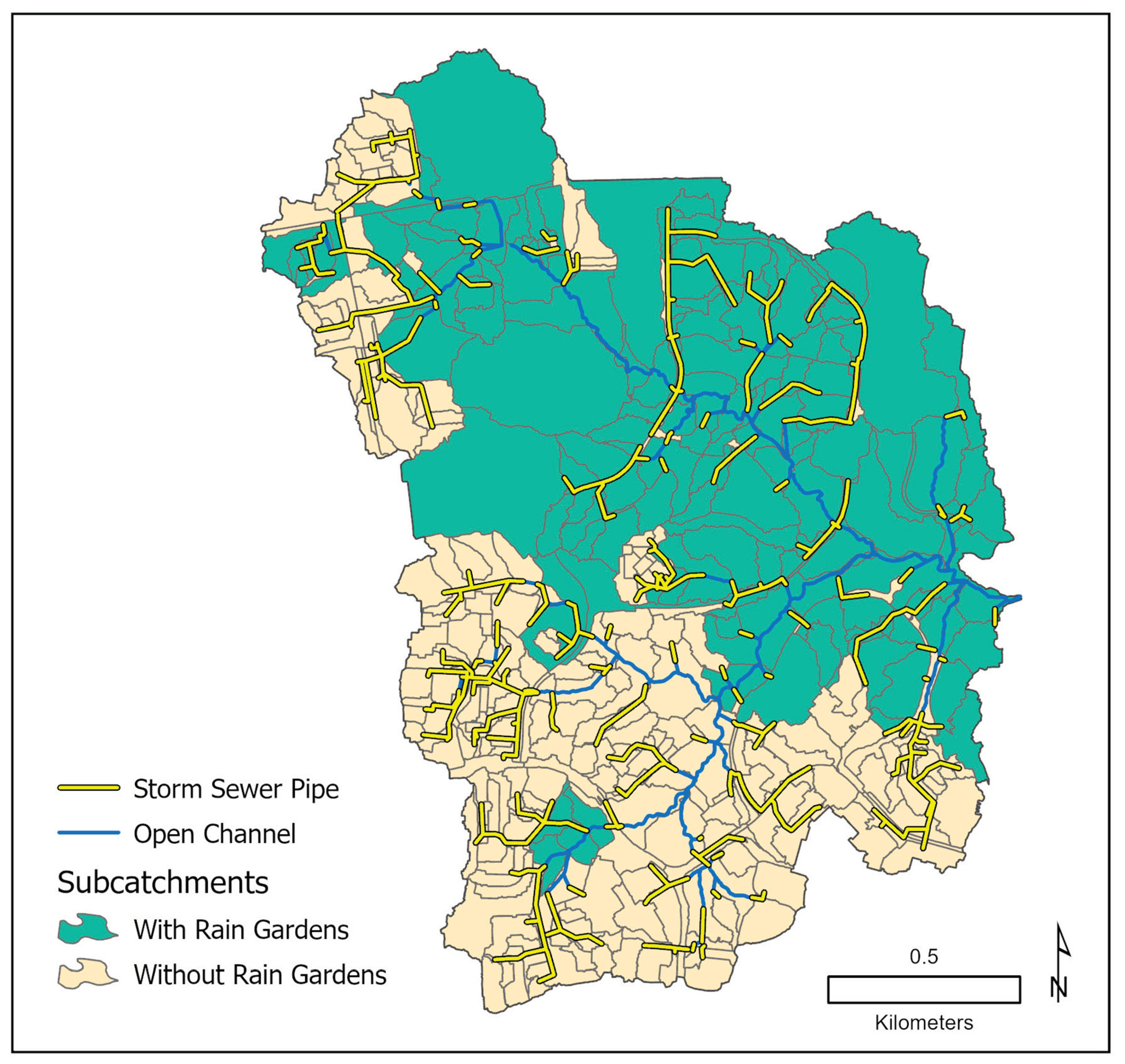
Watershed delineation and model parameterization were conducted using ArcGIS Pro [55]. The study catchment was discretized into 382 subcatchments based on topography, location of storm drains, and building rooftop pitch and downspout locations. Subcatchment areas ranged from 0.02 ha to 11.44 ha, with a median of 0.48 ha. To parameterize the model, GIS spatial analyses were conducted based on acquired data layers (Table 1) to determine the subcatchment physical characteristics required by SWMM, including area, characteristic width (i.e., width of overland flow), percent impervious, percent slope, roughness coefficient and depression storage for pervious and impervious areas, and infiltration parameters (i.e., saturated hydraulic conductivity, suction head, and initial moisture deficit). Storm sewer locations and parameters, including pipe length, slope, cross-section, and roughness, were gleaned from storm drain infrastructure design and as-built drawings (Figure 2). In the case of several inlets and manholes, there were data gaps in the available storm sewer drawings, and field visits were required to measure pipe sizes and storm drain inlet depths. Stream channel geometries were derived from channel topographic cross-sections using PCSWMM’s transect creator tool.
Infiltration was simulated using SWMM’s Modified Green-Ampt model. The Green-Ampt equation is more physically-based than other infiltration estimation methods, and the Modified Green-Ampt method adjusts the original Green-Ampt procedure by not depleting moisture deficit in the top surface layer of soil during initial periods of low rainfall [52,64]. This method can produce more realistic infiltration behavior for storm events with long initial periods during which the rainfall intensity is below the soil’s saturated hydraulic conductivity [52]. The dynamic wave method was used for hydraulic routing due to its ability to simulate non-uniform, unsteady state flow conditions. SWMM uses the Hargreaves method to simulate evaporation based on a daily minimum and maximum temperature time series and the catchment’s latitude [54,65].
The model was calibrated using two years of observed discharge at a one-minute time-step at the catchment outlet, 5-min rainfall data from a rain gage 0.75 km (0.47 mi) from the catchment boundary, and temperature data (daily minima and maxima) from an observation station 0.98 km (0.61 mi) from the catchment boundary. A sensitivity analysis was performed using PCSWMM’s Sensitivity-based Radio Tuning Calibration (SRTC) tool, which runs the model repeatedly, varying the values of selected parameters based on user-defined uncertainty ranges, and displays the ranked sensitivity of an objective function (e.g., peak flow) to the parameters. The selected calibration parameters were the seven most sensitive subcatchment attributes: characteristic width (a proxy for subcatchment shape), percent impervious, saturated hydraulic conductivity, depression storage for pervious areas, Manning’s roughness for pervious areas, suction head, and percent slope. Although SWMM can simulate groundwater flow based on aquifer parameters, calibration results were improved when the groundwater process model was turned off, so groundwater flow was not simulated. The calibration period was water years 2019-2020, and the Nash-Sutcliffe Efficiency (NSE, a commonly used statistic for assessing the goodness-of-fit of hydrologic models) after calibration was 0.766 [66]. Values of the NSE closer to 1 indicate a model with more predictive power; models with values of NSE between 0.7 and 0.8 are commonly classified as “satisfactory” [67,68]. The calibrated model was validated against one year of observed discharge (water year 2021), for which the NSE was 0.711. Based on evaluations of model performance criteria in the literature, the model was considered satisfactory [68].

2.3. Rain Garden Scenario Simulations

To test the effects of varying extents of residential rain garden implementation on event runoff, multiple scenarios were created in SWMM to represent the treatment of detached house rooftops by rain gardens. SWMM allows the user to explicitly simulate the performance of low impact development and green infrastructure (LID-GI) practices, including rain gardens. A rain garden (RG) is defined by SWMM as a bioretention cell without a storage layer (i.e., a gravel bed) or underdrain, and thus has only a vegetated surface layer and a soil layer. Runoff from RGs is estimated by a mass balance equation consisting of inputs (run-on and direct precipitation) and outputs (infiltration, evapotranspiration, and overflow). To test the effects on event hydrology of retrofitting of residential houses with RGs in the study catchment, four RG implementation scenarios were modeled. These included 25%, 50%, 75%, and 100% implementation scenarios, which correspond to one quarter, one half, three quarters, and the entirety of the rooftop area of all detached single-family houses in the catchment draining to RGs, respectively.
A generic RG was parameterized and duplicated for use in the RG scenario simulations. RG attributes were based on both reference values and previous RGs installed in the Columbia, MD [69]. The following values were used for the surface layer in a RG: a berm height of 102 mm, a vegetation volume fraction of 0.1, a Manning’s roughness coefficient of 0.3, and a surface slope of 0.25%. The following values were used for the soil layer: thickness of 889 mm, porosity of 0.44, field capacity of 0.11, wilting point of 0.05, hydraulic conductivity of 25 mm/hr, conductivity slope (average slope of log of conductivity versus soil moisture deficit curve) of 7.5, and a suction head of 89 mm. These values are consistent with those given in Rossman & Huber [69] and Avellaneda et al. [25]. RG area was set to 20.9 m2, which can treat approximately 43.3 m2 of rooftop, or one quarter of the average detached house rooftop area in the study catchment. Thus, the average detached house in the study catchment would be treated by exactly four RGs. In the 100% RG implementation scenario, 2,985 RGs covering an area of 6.2 ha were installed to treat 746 houses in 137 subcatchments (Figure 2).
A three-year simulation period was used in the scenario simulations (water years 2016-2018). There were 365 rainfall events in the simulation period, identified using a minimum inter-event time of 6 hours (rainfall occurring more than 6 hours after the previous rainfall constituted a new event). These events were filtered to 224 events that generated significant runoff in the baseline scenario, i.e., those producing peak flows greater than 0.057 cubic meters per second (cms) (2 cubic feet per second [cfs]). One of these events was removed as an outlier because it produced a double hydrograph peak that led to erroneous peak flow reduction and lag time increase calculations, leaving a sample of 223 runoff events for analysis. For each of these events, peak flow, event runoff volume, and time of peak flow were calculated from the simulated hydrographs. From these data, peak flow reductions, runoff volume reductions, and lag time increases were calculated for all events in each experimental scenario, relative to the baseline scenario. Lag time was calculated as the time from rainfall centroid to peak discharge (centroid lag-to-peak). To evaluate the difference between the sets of paired hydrologic metrics (before and after RG implementation), one-sided Wilcoxon Signed Rank Tests for paired samples were performed in R. The non-parametric paired difference hypothesis test was employed because it could not be assumed that the populations of variable values were normally distributed. The tests were one-sided because it was expected that the median differences in peak flows, event runoff volumes, and times of peak flow between the baseline and RG implementation scenarios were, respectively, a decrease, a decrease, and an increase. The null hypothesis was that the median difference between the two populations was zero, with an alpha value threshold for significance of 0.05. Additionally, linear regression was used to test whether rainfall depth had a relationship with each of the runoff parameters of peak flow, event runoff volume, and lag time.

3. Results

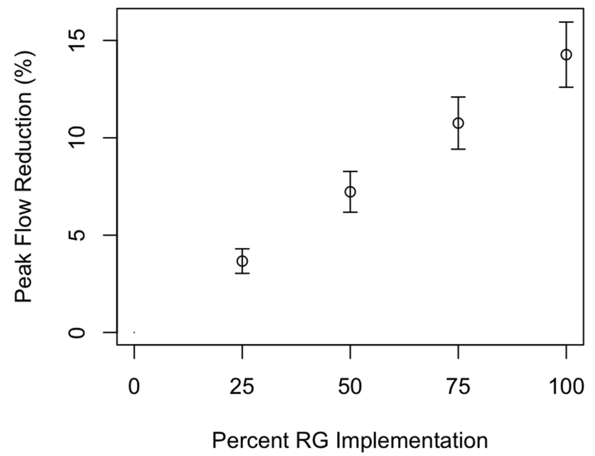
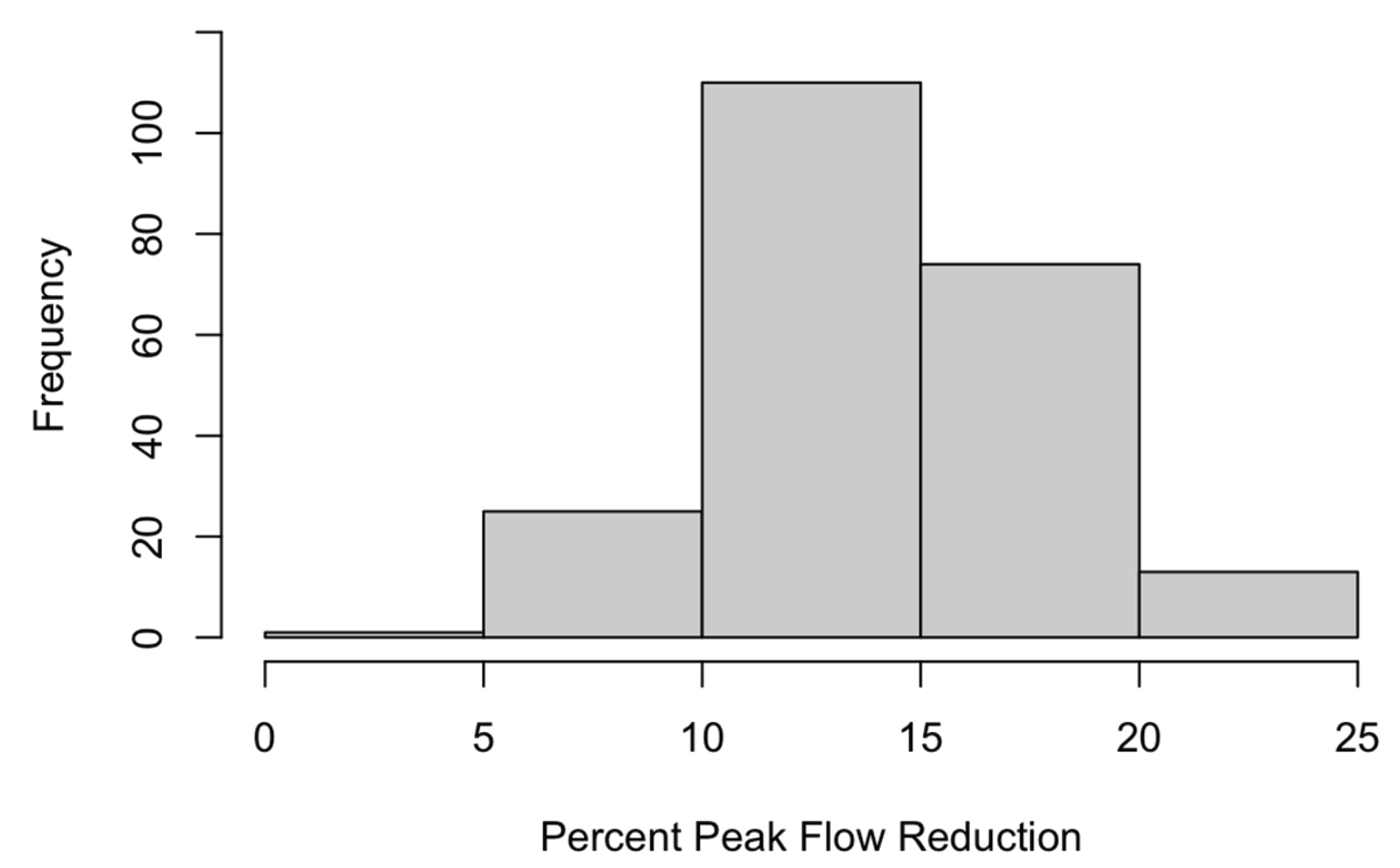
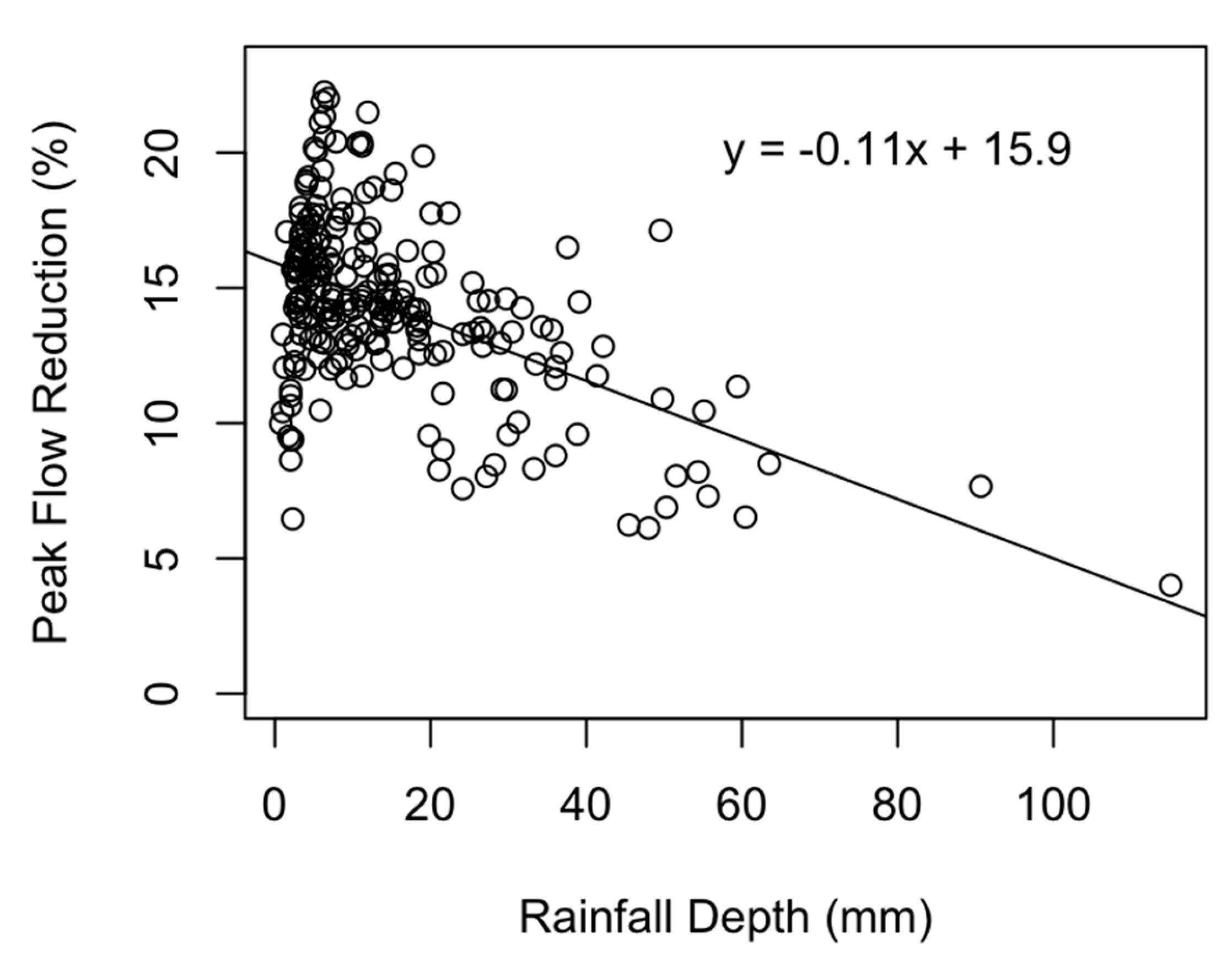
For each of the four rain garden scenarios (25%, 50%, 75%, and 100%), differences in peak flow, stormflow volume, and time of peak flow between the 223 matched events were found to be statistically significant (p<0.01) for all RG implementation scenarios. Mean peak flow reductions (PFRs) for the 25%, 50%, 75%, and 100% RG implementation scenarios were 3.6%, 7.2%, 10.8%, and 14.3%, respectively (Figure 3). For the 100% RG implementation scenario, PFRs ranged from 4.0% to 22.2% (Figure 4). For only the 18 events with rainfall depths >38.1 mm (1.5 in), mean PFR in the 100% RG implementation scenario was reduced to 9.3%, while for the 131 events with rainfall depths <12.7 mm (0.5 in), mean PFR increased to 15.4%. Peak flow reduction (PFR) was inversely correlated with rainfall depth (p<0.01) (Figure 5).
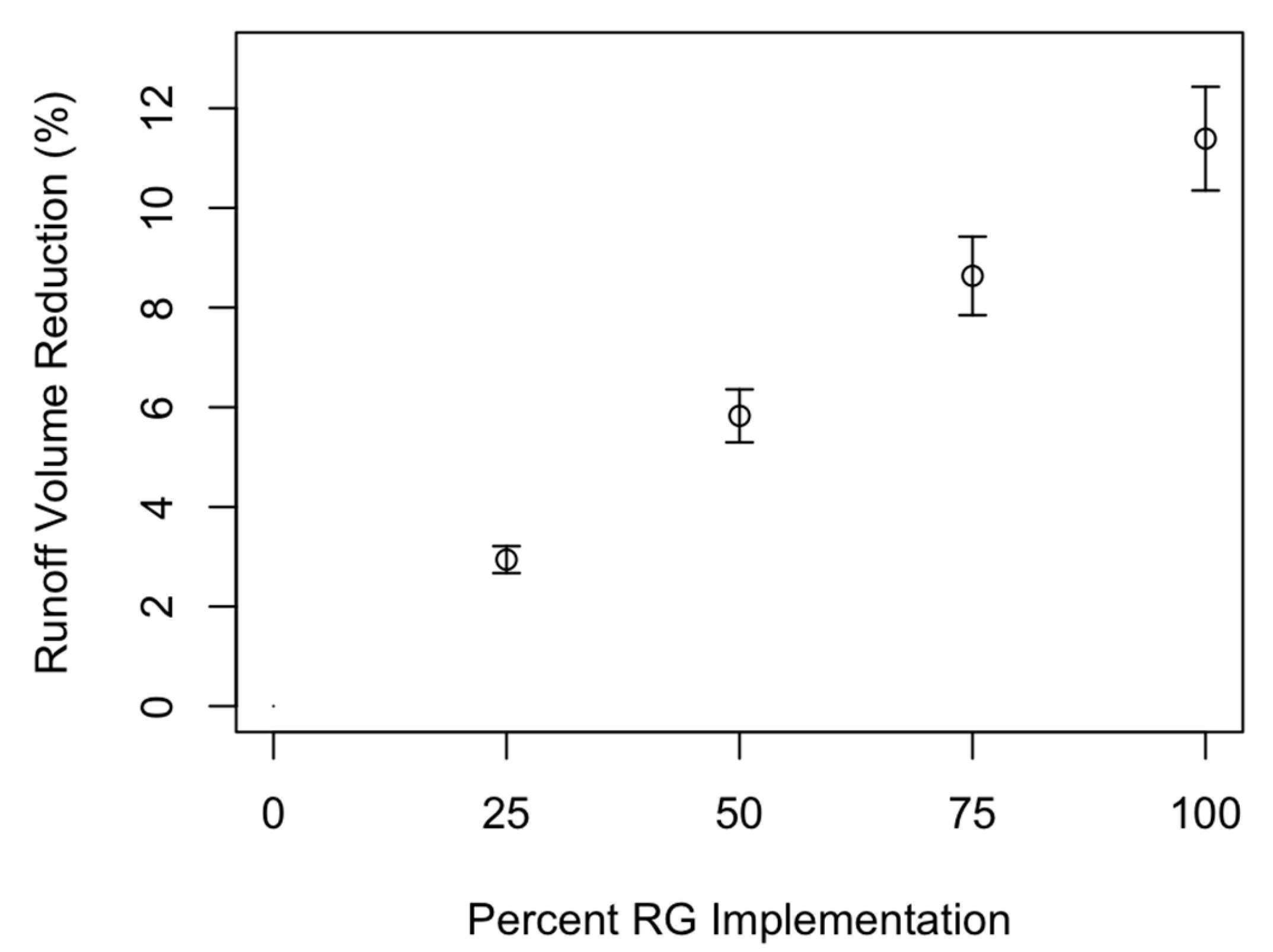
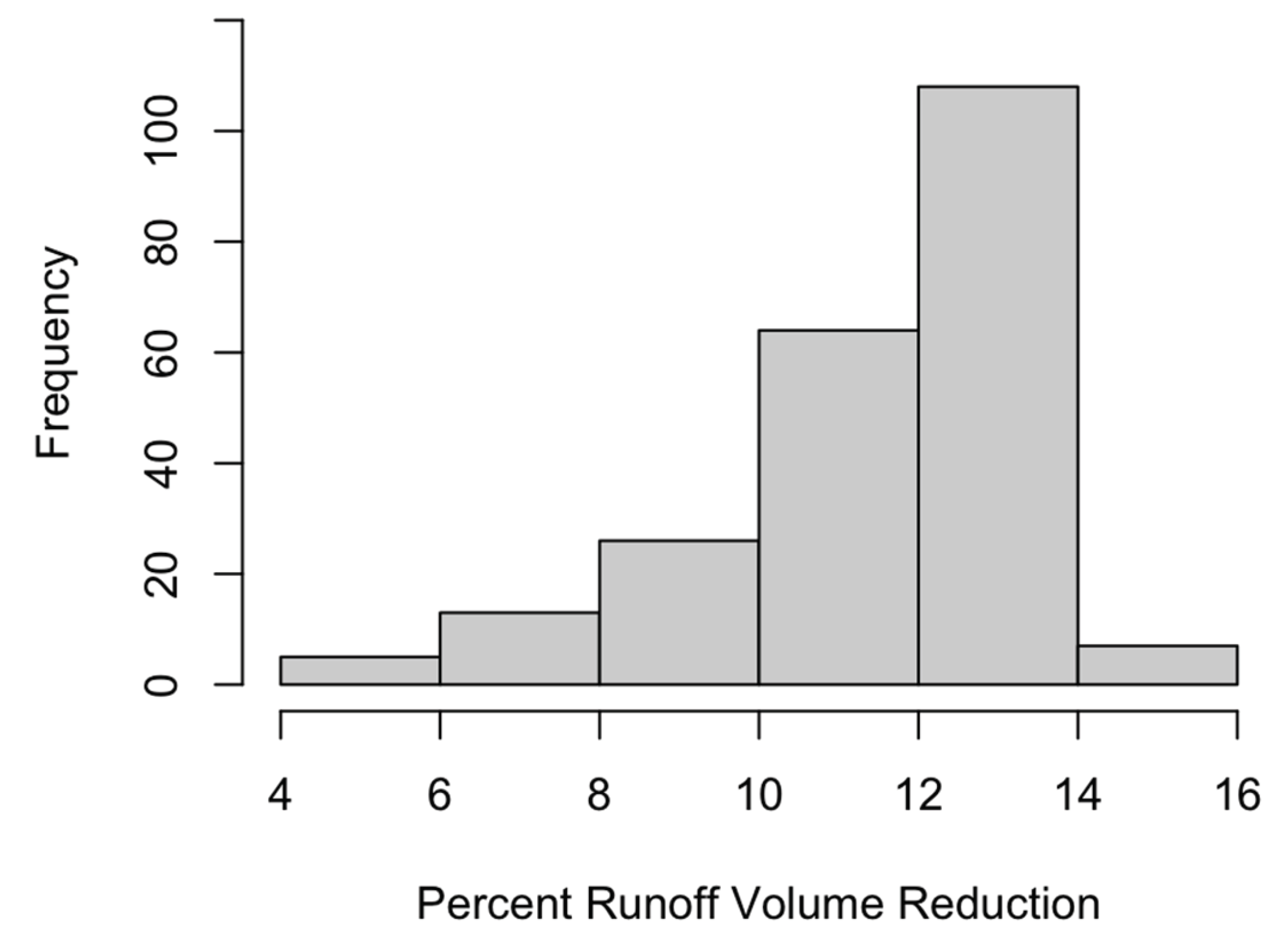
Mean event runoff volume reductions (RVRs) for the 25%, 50%, 75%, and 100% RG implementation scenarios were 2.9%, 5.8%, 8.6%, and 11.4%, respectively (Figure 6). For the 100% RG implementation scenario, RVRs ranged from 4.2% to 14.5% (Figure 7). For events with rainfall depths >38.1 mm (1.5 in), mean RVR in the 100% RG implementation scenario was 10.5%, while for events with rainfall depths <12.7 mm (0.5 in), mean RVR was 11.1%. A regression analysis did not find a significant linear relationship between runoff volume reduction and rainfall depth.
The mean lag time (centroid lag-to-peak) for the 223 events in the baseline scenario was 1 hour and 16 minutes. This lag time was increased in the 25%, 50%, 75%, and 100% RG implementation scenarios by <1 min, 1.4 min, 1.9 min, and 2.4 min, respectively.
Overall, for the smallest level of rain garden implementation at 25%, corresponding to 3.3% of total impervious area (TIA) treated in this 3.1 km2 catchment, we found that event runoff improved by a mean reduction of peak flow of 3.6%, and a mean reduction in runoff volume of 2.9%. For full implementation of residential rain gardens at the 100% level (or 13.1% of TIA), we found that, on average, peak flows were reduced by 14.3%, runoff volumes were reduced by 11.4%, and times of peak flow were delayed by 3.2%.

4. Discussion

The simulation results indicated that rain garden implementation can significantly reduce peak flows and runoff volumes, and increase lag times, even when implemented at only 25% of detached house rooftops. Treating 100% of residential rooftops in the catchment (4.1% of the catchment area and 13.1% of total impervious area [TIA]) could reduce peak flows by up 22.2%, and runoff volumes by up to 14.5%. Mean reductions in peak flow and runoff volume were greater for smaller storm events, and peak flow reduction was linearly related to rainfall depth (p<0.01). These results are consistent with those of Samouei and Özger [37], who found in a simulation study that treating 10% of TIA with various LID-GI practices including bioretention cells in a 1.05 km2 catchment reduced peak flows and runoff volumes from the 2-year storm by 12% and 8%, respectively. In another modeling study, Hoghooghi et al. [70] found that implementing a 0.94 km2 mixed suburban, agricultural, and forested watershed with rain gardens and other LID-GI practices reduced peak flow and surface runoff of 8.5% and 8.0%, respectively. Based on a statistical relationship between percent TIA treated and catchment-scale LID-GI hydrologic performance developed in a meta-analysis by Bell et al. [17], if 13.1% of TIA was redirected to rain gardens (as in the 100% RG implementation scenario), peak flows and event runoff would be expected to be reduced by 7.9% and 5.6%, respectively. The rain garden performance simulated in this study were generally consistent with those observed in previous, similar investigations, and bear out the findings that percent peak flow reductions typically exceed runoff volume reductions, and that performance diminishes with increasing storm depth. This study is distinguished by its scale, level of detail (382 subcatchments), its use of continuous rather than event-based simulations, and its focus on residential rain gardens in suburban areas.
Simulated lag time increases (2.4 minutes on average for the 100% implementation scenario) were consistent with those of Palla and Gnecco [71], who developed a SWMM model of a 5.5 ha catchment and found that treating up to 36% of effective impervious area (EIA) with green roofs and permeable pavement increased lag times from the 2-year storm by ~3 minutes. The lag time increases in the present study were smaller than those observed by Li et al. [72], who used SWMM to model the effects of rain garden implementation in a 16.5 km2 highly urbanized catchment, and found that treating 4% of the catchment delayed peak flows from the 2-year storm by up to 7 minutes. In general, the results of the present study support the prior body of evidence that implementation of LID-GI such as rain gardens can result in modest but statistically significant increases in lag time. Few if any previous studies, however, have specifically examined the catchment-scale performance of residential rain gardens in suburban basins of this size.
Like other modeling investigations of LID-GI hydrologic performance, the present study is limited by some assumptions and simplifications. For example, as a lumped (semi-distributed) hydrologic model, SWMM is based on the assumption that physical characteristics within each subcatchment (e.g., soil type and surface slope) are uniform [52]. We addressed this limitation to some extent by our fine-scaled delineation of subcatchments, with each selected to group together similar topographic and land use characteristics within the hydrologic network of the study area. For this study specifically, the SWMM model did not explicitly represent floodplain storage, snowmelt, or groundwater contributions to stream discharge, although as in many small, urban watersheds, these contributions were deemed to have minimal impacts on event flow indices [73]. The extensive calibration and validation periods showed that the model as implemented satisfactorily matched observed streamflow at the outlet USGS streamgage. Additionally, temporal variations in rain garden functioning were ignored, such as deterioration in performance due to clogging, vegetation change, or lack of maintenance, which could lead to over-estimation of long-term catchment-scale effectiveness [15].
This study addressed an important research gap in the literature by investigating the catchment-scale effectiveness of residential rain gardens in an intermediate-sized suburban catchment. Moreover, the present study was notable for its fine scale and level of detail, with the model containing 382 subcatchments, and explicitly representing 473 storm sewer inlets and manholes in a catchment area of only 3.1 km2. Future research should examine the effects of varying the spatial distribution of rain gardens on their cumulative performance, as well as temporal factors such as seasonal variation in antecedent moisture conditions, soil distributions and disruptions in urban settings, and non-stationarity of climate variables. As watershed managers increasingly look to LID-GI approaches to address the compounding effects of urbanization and climate change on water quality and quantity, the results of this study indicate that residential rain gardens can significantly improve the runoff response of suburban catchments, and are an effective tool for improving stormwater management in residential areas.

Author Contributions

Conceptualization, B.J.D. and J.A.Y.; methodology, B.J.D. and J.A.Y; software, B.J.D..; formal analysis, B.J.D.; writing—original draft preparation, B.J.D.; writing—review and editing, B.J.D. and J.A.Y; visualization, B.J.D.; supervision, J.A.Y.; project administration, J.A.Y. All authors have read and agreed to the published version of the manuscript.

Funding

This research received no external funding.

Data Availability Statement

The raw data supporting the conclusions of this article will be made available by the authors on request.

Acknowledgments

The authors gratefully acknowledge David Sample for his assistance in model development, David Poltilove for collecting and providing daily temperature data, and the Howard County Stormwater Management Division for providing storm drain infrastructure data.

Conflicts of Interest

The authors declare no conflicts of interest.

References

  1. Hughes, R.M.; Dunham, S.; Maas-Hebner, K.G.; Yeakley, J.A.; Schreck, C.; Harte, M.; Molina, N.; Shock, C.C.; Kaczynski, V.W.; Schaeffer, J. A Review of Urban Water Body Challenges and Approaches: (1) Rehabilitation and Remediation. Fisheries 2014, 39, 18–29. [Google Scholar] [CrossRef]
  2. Walsh, C.J.; Roy, A.H.; Feminella, J.W.; Cottingham, P.D.; Groffman, P.M.; Morgan, R.P. The Urban Stream Syndrome: Current Knowledge and the Search for a Cure. J. North Am. Benthol. Soc. 2005, 24, 706–723. [Google Scholar] [CrossRef]
  3. Walsh, C.J.; Fletcher, T.D.; Burns, M.J. Urban Stormwater Runoff: A New Class of Environmental Flow Problem. PLoS ONE 2012, 7, e45814. [Google Scholar] [CrossRef] [PubMed]
  4. Leopold, L. Hydrology for Urban Land Planning – A Guidebook on the Hydrologic Effects of Urban Land Use; U.S. Geological Survey: Washington, D.C., 1968.
  5. Paul, M.J.; Meyer, J.L. Streams in the Urban Landscape. Annu. Rev. Ecol. Syst. 2001, 32, 333–365. [Google Scholar] [CrossRef]
  6. Ahiablame, L.M.; Engel, B.A.; Chaubey, I. Effectiveness of Low Impact Development Practices: Literature Review and Suggestions for Future Research. Water Air Soil Pollut. 2012, 223, 4253–4273. [Google Scholar] [CrossRef]
  7. Dietz, M.E. Low Impact Development Practices: A Review of Current Research and Recommendations for Future Directions. Water Air Soil Pollut. 2007, 186, 351–363. [Google Scholar] [CrossRef]
  8. U.S. Environmental Protection Agency (USEPA) What Is Green Infrastructure? Available online: https://www.epa.gov/green-infrastructure/what-green-infrastructure (accessed on 16 March 2024).
  9. Anderson, A.R.; Franti, T.G.; Shelton, D.P. Hydrologic Evaluation of Residential Rain Gardens Using a Stormwater Runoff Simulator. Trans. ASABE 2018, 61, 495–508. [Google Scholar] [CrossRef]
  10. Davis, A.P. Field Performance of Bioretention: Hydrology Impacts. J. Hydrol. Eng. 2008, 13, 90–95. [Google Scholar] [CrossRef]
  11. Shuster, W.; Darner, R.; Schifman, L.; Herrmann, D. Factors Contributing to the Hydrologic Effectiveness of a Rain Garden Network (Cincinnati OH USA). Infrastructures 2017, 2, 11. [Google Scholar] [CrossRef] [PubMed]
  12. Tu, M.-C.; Traver, R. Water Table Fluctuation from Green Infrastructure Sidewalk Planters in Philadelphia. J. Irrig. Drain Eng. 2019, 145, 05018008. [Google Scholar] [CrossRef]
  13. Golden, H.E.; Hoghooghi, N. Green Infrastructure and Its Catchment-Scale Effects: An Emerging Science. Wiley Interdiscip. Rev. : Water 2018, 5, e1254. [Google Scholar] [CrossRef] [PubMed]
  14. Jefferson, A.J.; Bhaskar, A.S.; Hopkins, K.G.; Fanelli, R.; Avellaneda, P.M.; McMillan, S.K. Stormwater Management Network Effectiveness and Implications for Urban Watershed Function: A Critical Review. Hydrol. Process. 2017, 31, 4056–4080. [Google Scholar] [CrossRef]
  15. Li, C.; Fletcher, T.D.; Duncan, H.P.; Burns, M.J. Can Stormwater Control Measures Restore Altered Urban Flow Regimes at the Catchment Scale? J. Hydrol. 2017, 549, 631–653. [Google Scholar] [CrossRef]
  16. Jennings, A.A.; Berger, M.A.; Hale, J.D. Hydraulic and Hydrologic Performance of Residential Rain Gardens. J. Environ. Eng. 2015, 141, 04015033. [Google Scholar] [CrossRef]
  17. Bell, C.D.; Wolfand, J.M.; Panos, C.L.; Bhaskar, A.S.; Gilliom, R.L.; Hogue, T.S.; Hopkins, K.G.; Jefferson, A.J. Stormwater Control Impacts on Runoff Volume and Peak Flow: A Meta-analysis of Watershed Modelling Studies. Hydrol. Process. 2020, 34, 3134–3152. [Google Scholar] [CrossRef]
  18. Hopkins, K.G.; Bhaskar, A.S.; Woznicki, S.A.; Fanelli, R.M. Changes in Event-based Streamflow Magnitude and Timing after Suburban Development with Infiltration-based Stormwater Management. Hydrol. Process. 2020, 34, 387–403. [Google Scholar] [CrossRef] [PubMed]
  19. Jarden, K.M.; Jefferson, A.J.; Grieser, J.M. Assessing the Effects of Catchment-Scale Urban Green Infrastructure Retrofits on Hydrograph Characteristics. Hydrol. Process. 2016, 30, 1536–1550. [Google Scholar] [CrossRef]
  20. Loperfido, J.V.; Noe, G.B.; Jarnagin, S.T.; Hogan, D.M. Effects of Distributed and Centralized Stormwater Best Management Practices and Land Cover on Urban Stream Hydrology at the Catchment Scale. J. Hydrol. 2014, 519, 2584–2595. [Google Scholar] [CrossRef]
  21. Pennino, M.J.; McDonald, R.I.; Jaffe, P.R. Watershed-Scale Impacts of Stormwater Green Infrastructure on Hydrology, Nutrient Fluxes, and Combined Sewer Overflows in the Mid-Atlantic Region. Sci. Total Environ. 2016, 565, 1044–1053. [Google Scholar] [CrossRef] [PubMed]
  22. Rhea, L.; Jarnagin, T.; Hogan, D.; Loperfido, J.V.; Shuster, W. Effects of Urbanization and Stormwater Control Measures on Streamflows in the Vicinity of Clarksburg, Maryland, USA: Effects on Streamflows. Hydrol. Process. 2015, 29, 4413–4426. [Google Scholar] [CrossRef]
  23. Shuster, W.; Rhea, L. Catchment-Scale Hydrologic Implications of Parcel-Level Stormwater Management (Ohio USA). J. Hydrol. 2013, 485, 177–187. [Google Scholar] [CrossRef]
  24. Woznicki, S.A.; Hondula, K.L.; Jarnagin, S.T. Effectiveness of Landscape-Based Green Infrastructure for Stormwater Management in Suburban Catchments. Hydrol. Process. 2018, 32, 2346–2361. [Google Scholar] [CrossRef]
  25. Avellaneda, P.M.; Jefferson, A.J.; Grieser, J.M.; Bush, S.A. Simulation of the Cumulative Hydrological Response to Green Infrastructure. Water Resour. Res. 2017, 53, 3087–3101. [Google Scholar] [CrossRef]
  26. Rezaei, A.R.; Ismail, Z.; Niksokhan, M.H.; Dayarian, M.A.; Ramli, A.H.; Shirazi, S.M. A Quantity–Quality Model to Assess the Effects of Source Control Stormwater Management on Hydrology and Water Quality at the Catchment Scale. Water 2019, 11, 1415. [Google Scholar] [CrossRef]
  27. Avellaneda, P.M.; Jefferson, A.J. Sensitivity of Streamflow Metrics to Infiltration-Based Stormwater Management Networks. Water Resour. Res. 2020, 56. [Google Scholar] [CrossRef]
  28. Boening-Ulman, K.M.; Winston, R.J.; Wituszynski, D.M.; Smith, J.S.; Andrew Tirpak, R.; Martin, J.F. Hydrologic Impacts of Sewershed-Scale Green Infrastructure Retrofits: Outcomes of a Four-Year Paired Watershed Monitoring Study. J. Hydrol. 2022, 611, 128014. [Google Scholar] [CrossRef]
  29. Feng, M.; Jung, K.; Li, F.; Li, H.; Kim, J.-C. Evaluation of the Main Function of Low Impact Development Based on Rainfall Events. Water 2020, 12, 17. [Google Scholar] [CrossRef]
  30. Hood, M.J.; Clausen, J.C.; Warner, G.S. Comparison of Stormwater Lag Times for Low Impact and Traditional Residential Development. J Am Water Resour. Assoc 2007, 43, 1036–1046. [Google Scholar] [CrossRef]
  31. Lammers, R.W.; Miller, L.; Bledsoe, B.P. Effects of Design and Climate on Bioretention Effectiveness for Watershed-Scale Hydrologic Benefits. J. Sustain. Water Built Environ. 2022, 8, 04022011. [Google Scholar] [CrossRef]
  32. Ahiablame, L.; Shakya, R. Modeling Flood Reduction Effects of Low Impact Development at a Watershed Scale. J. Environ. Manag. 2016, 171, 81–91. [Google Scholar] [CrossRef]
  33. Epps, T.H.; Hathaway, J.M. Using Spatially-Identified Effective Impervious Area to Target Green Infrastructure Retrofits: A Modeling Study in Knoxville, TN. J. Hydrol. 2019, 575, 442–453. [Google Scholar] [CrossRef]
  34. Di Vittorio, D.; Ahiablame, L. Spatial Translation and Scaling Up of Low Impact Development Designs in an Urban Watershed. J. Water Manag. Model. 2015. [Google Scholar] [CrossRef]
  35. Fan, G.; Lin, R.; Wei, Z.; Xiao, Y.; Shangguan, H.; Song, Y. Effects of Low Impact Development on the Stormwater Runoff and Pollution Control. Sci. Total Environ. 2022, 805, 150404. [Google Scholar] [CrossRef] [PubMed]
  36. Liang, C.-Y.; You, G.J.-Y.; Lee, H.-Y. Investigating the Effectiveness and Optimal Spatial Arrangement of Low-Impact Development Facilities. J. Hydrol. 2019, 577, 124008. [Google Scholar] [CrossRef]
  37. Samouei, S.; Özger, M. Evaluating the Performance of Low Impact Development Practices in Urban Runoff Mitigation through Distributed and Combined Implementation. J. Hydroinformatics 2020, 22, 1506–1520. [Google Scholar] [CrossRef]
  38. Wadhwa, A.; Pavan Kumar, K. Selection of Best Stormwater Management Alternative Based on Storm Control Measures (SCM) Efficiency Indices. Water Policy 2020, 22, 702–715. [Google Scholar] [CrossRef]
  39. Zhang, L.; Ye, Z.; Shibata, S. Assessment of Rain Garden Effects for the Management of Urban Storm Runoff in Japan. Sustainability 2020, 12, 9982. [Google Scholar] [CrossRef]
  40. Li, J.; Zhang, B.; Li, Y.; Li, H. Simulation of Rain Garden Effects in Urbanized Area Based on Mike Flood. Water 2018, 10, 860. [Google Scholar] [CrossRef]
  41. Guo, X.; Du, P.; Zhao, D.; Li, M. Modelling Low Impact Development in Watersheds Using the Storm Water Management Model. Urban Water J. 2019, 16, 146–155. [Google Scholar] [CrossRef]
  42. Hopkins, K.G.; Woznicki, S.A.; Williams, B.M.; Stillwell, C.C.; Naibert, E.; Metes, M.J.; Jones, D.K.; Hogan, D.M.; Hall, N.C.; Fanelli, R.M.; et al. Lessons Learned from 20 y of Monitoring Suburban Development with Distributed Stormwater Management in Clarksburg, Maryland, USA. Freshw. Sci. 2022, 000–000. [Google Scholar] [CrossRef]
  43. Page, J.L.; Winston, R.J.; Mayes, D.B.; Perrin, C.A.; Hunt, W.F. Retrofitting Residential Streets with Stormwater Control Measures over Sandy Soils for Water Quality Improvement at the Catchment Scale. J. Environ. Eng. 2015, 141, 04014076. [Google Scholar] [CrossRef]
  44. Tchintcharauli-Harrison, M.B.; Santelmann, M.V.; Greydanus, H.; Shehab, O.; Wright, M. Role of Neighborhood Design in Reducing Impacts of Development and Climate Change, West Sherwood, OR. Front. Water 2022, 3, 757420. [Google Scholar] [CrossRef]
  45. Parker, K.; Horowitz, J.M.; Brown, A.; Fry, R.; Cohn, D.; Igielnik, R. Demographic and Economic Trends in Urban, Suburban and Rural Communities. Pew Research Center’s Social & Demographic Trends Project 2018.
  46. United Nations, Department of Economic and Social Affairs, Population Division (UN DESA) World Urbanization Prospects: The 2018 Revision; New York, 2019.
  47. IPCC Climate Change 2023: Synthesis Report; Contribution of Working Groups I, II and III to the Sixth Assessment Report of the Intergovernmental Panel on Climate Change [Core Writing Team, H. Lee and J. Romero (eds.)]; IPCC: Geneva, Switzerland, 2023.
  48. Howard County GIS Division Howard County, Maryland, Geologic Formations. Available online: https://data.howardcountymd.gov/mapgallery/misc/Geology22x34countywide.pdf (accessed on 21 March 2024).
  49. U.S. Climate Data Weather Averages Baltimore-BWI Arpt, Maryland. Available online: https://www.usclimatedata.com/climate/baltimore-bwi-arpt/maryland/united-states/usmd0019 (accessed on 22 February 2024).
  50. National Water Information System (NWIS) USGS Current Conditions for USGS 01593370 L PAX RIV TRIB ABOVE WILDE LAKE AT COLUMBIA, MD. Available online: https://waterdata.usgs.gov/nwis/uv?site_no=01593370 (accessed on 22 February 2024).
  51. Center for Watershed Protection and Tetra Tech, Inc. Centennial and Wilde Lake Watershed Restoration Plan; 2005. Available online: https://www.howardcountymd.gov/sites/default/files/media/2015-12/Section1_Introduction.pdf (accessed on 22 February 2024).
  52. Rossman, L.A. Storm Water Management Model User’s Manual Version 5.1; U.S. Environmental Protection Agency, 2015.
  53. CHI Computational Hydraulics International (CHI). Available online: https://www.chiwater.com/Home (accessed on 4 February 2024).
  54. Rossman, L.A.; Huber, W. Storm Water Management Model Reference Manual Volume I – Hydrology (Revised); U.S. Environmental Protection Agency: Cincinnati, OH, 2016.
  55. ESRI Desktop GIS Software | Mapping Analytics | ArcGIS Pro. Available online: https://www.esri.com/en-us/arcgis/products/arcgis-pro/overview (accessed on 4 February 2024).
  56. U.S. Geological Survey (USGS) The National Map Downloader. Available online: https://apps.nationalmap.gov/downloader/ (accessed on 26 March 2024).
  57. U.S. Geological Survey (USGS) EarthExplorer. Available online: https://earthexplorer.usgs.gov/ (accessed on 26 March 2024).
  58. Maryland Geographic Information Office MD iMAP Portal. Available online: https://imap.maryland.gov/ (accessed on 26 March 2024).
  59. Howard County GIS Division Howard County Maryland Data Download and Viewer. Available online: https://data.howardcountymd.gov/ (accessed on 26 March 2024).
  60. U.S. Department of Agriculture Natural Resources Conservation Service Web Soil Survey Available online: https://websoilsurvey.nrcs.usda.gov/app/WebSoilSurvey.aspx (accessed on 26 March 2024).
  61. Wijetunge, R. Storm Drain Infrastructure Data (Howard County Government Stormwater Management Division), personal communication, 22 June 2022.
  62. Baltimore County Dept. of Public Works Baltimore County Rain Gauge Data Available online: https://drive.google.com/drive/folders/1ZP_kHl_bdiL6JMYuXUDT_5GXTzwq2KHM (accessed 26 March 2024).
  63. Poltilove, D. Weather Data, personal communication, 9 September 2023.
  64. Green, W.; Ampt, G. Studies on Soil Physics, 1. The Flow of Air and Water Through Soils. J. Agric. Sci. 1911, 4, 11–24. [Google Scholar]
  65. Hargreaves, G.; Samani, Z. Reference Crop Evapotranspiration from Temperature. Appl. Eng. Agric. 1985, 1, 96–99. [Google Scholar] [CrossRef]
  66. Nash, J.E.; Sutcliffe, J.V. River Flow Forecasting through Conceptual Models Part I — A Discussion of Principles. J. Hydrol. 1970, 10, 282–290. [Google Scholar] [CrossRef]
  67. Ladson, A. Hydrology: An Australian Introduction; Oxford University Press Australia, 2008; ISBN 978-0-19-555358-1.
  68. Moriasi, *!!! REPLACE !!!*; Gitau, M.; Pai, N.; Daggupati, P. Hydrologic and Water Quality Models: Performance Measures and Evaluation Criteria. Trans. ASABE 2015, 58, 1763–1785. [Google Scholar] [CrossRef]
  69. Rossman, L.A.; Huber, W. Storm Water Management Model Reference Manual Volume III – Water Quality; U.S. Environmental Protection Agency: Cincinnati, OH, 2016; p. 127.
  70. Hoghooghi, N.; Golden, H.; Bledsoe, B.; Barnhart, B.; Brookes, A.; Djang, K.; Halama, J.; McKane, R.; Nietch, C.; Pettus, P. Cumulative Effects of Low Impact Development on Watershed Hydrology in a Mixed Land-Cover System. Water 2018, 10, 991. [Google Scholar] [CrossRef] [PubMed]
  71. Palla, A.; Gnecco, I. Hydrologic Modeling of Low Impact Development Systems at the Urban Catchment Scale. J. Hydrol. 2015, 528, 361–368. [Google Scholar] [CrossRef]
  72. Li, J.; Li, Y.; Li, Y. SWMM-Based Evaluation of the Effect of Rain Gardens on Urbanized Areas. Env. Earth Sci 2016, 75, 17. [Google Scholar] [CrossRef]
  73. Salvadore, E.; Bronders, J.; Batelaan, O. Hydrological Modelling of Urbanized Catchments: A Review and Future Directions. J. Hydrol. 2015, 529, 62–81. [Google Scholar] [CrossRef]
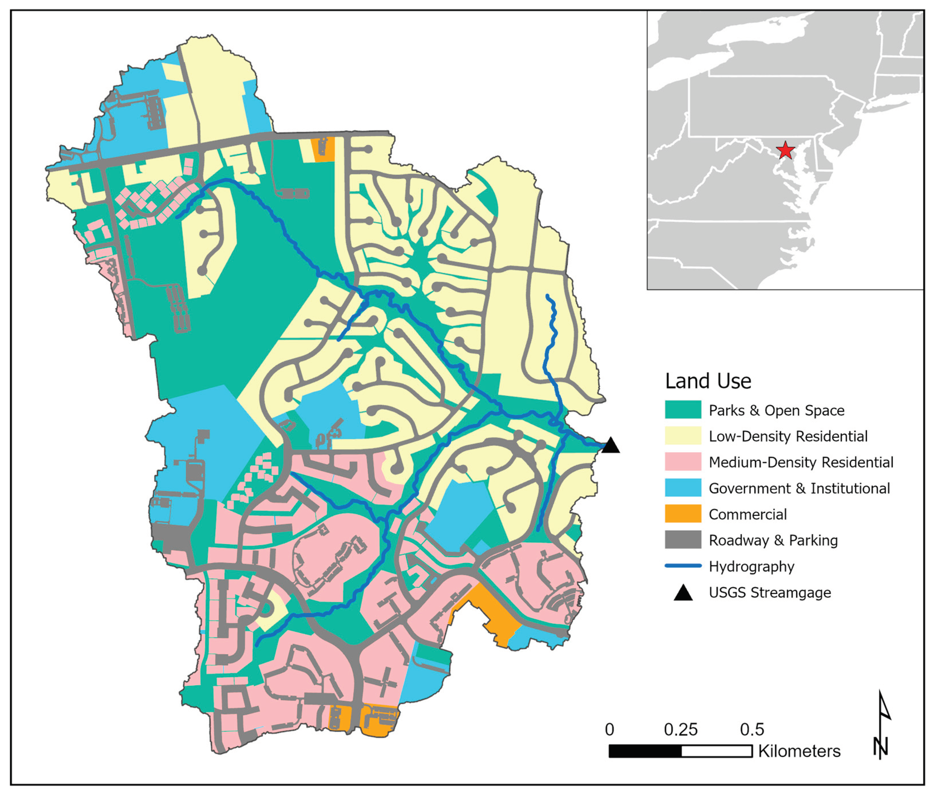
Figure 1. Study area location map and land use distribution.
Preprints 102646 g001
Figure 2. Conduits (storm sewer pipes and open channels) and subcatchments represented in the SWMM model. In the rain garden scenario simulations, subcatchments that contained any number of single-family detached houses (shown in green) were implemented with a proportional number of rain gardens.
Preprints 102646 g002
Figure 3. Mean peak flow reductions for the four rain garden (RG) scenario simulations. Error bars are one standard deviation.
Preprints 102646 g003
Figure 4. Histogram of percent peak flow reduction for the 100% rain garden implementation scenario (223 total events).
Preprints 102646 g004
Figure 5. Relationship between peak flow reduction and rainfall depth for the 223 rainfall events, with linear regression line (p<0.01).
Preprints 102646 g005
Figure 6. Mean runoff volume reductions for the four rain garden (RG) scenario simulations. Error bars are one standard deviation.
Preprints 102646 g006
Figure 7. Histogram of percent runoff volume reduction for the 100% rain garden implementation scenario (223 total events).
Preprints 102646 g007
Table 1. Data layers and sources used in model construction and parameterization.
Dataset or Layer Name Description Source
Digital Elevation Model (DEM) 1 meter DEM, dated 2018 USGS 3DEP Program, via USGS National Map Downloader [56]
Orthoimagery High-resolution (6-inch) aerial photography, dated 2014 and 2020 USGS Earth Explorer [57] and MD iMAP Portal [58]
Impervious Cover Dated 2020 Howard County Maryland Data Download and Viewer [59]
Land Use Dated 2024 Howard County Maryland Data Download and Viewer [59]
Forest Cover “Soft canopy” dated 2018 Howard County Maryland Data Download and Viewer [59]
Soil Data Characteristics for top 2 meters of soils Natural Resources Conservation Service (NRCS) Soil Survey Geographic Database (SSURGO) [60]
Storm Sewer Infrastructure Geodatabase containing inlet, manhole, pipe, and outfall locations Howard County Stormwater Management Division [61]
Rainfall 5-minute interval rainfall data Baltimore County Rain Gauge Network [62]
Temperature Daily maximum and minimum temperature Observation station operated by a Community Collaborative Rain, Hail, and Snow Network (CoCoRaHS) observer [63]
Discharge 1-minute interval discharge at the catchment outlet USGS streamgage 01593370, via the National Water Information System (NWIS) [50]
Disclaimer/Publisher’s Note: The statements, opinions and data contained in all publications are solely those of the individual author(s) and contributor(s) and not of MDPI and/or the editor(s). MDPI and/or the editor(s) disclaim responsibility for any injury to people or property resulting from any ideas, methods, instructions or products referred to in the content.
Copyright: This open access article is published under a Creative Commons CC BY 4.0 license, which permit the free download, distribution, and reuse, provided that the author and preprint are cited in any reuse.
Alerts
Prerpints.org logo

Preprints.org is a free preprint server supported by MDPI in Basel, Switzerland.

Subscribe

© 2025 MDPI (Basel, Switzerland) unless otherwise stated