1. Introduction
A fundamental problem in modelling is the estimation of unknown parameters from empirical data . Frequently however, practical situations require estimation of individual parameters for a large number of datasets. Fitting the same model to multiple datasets and extracting parameters specific for each dataset is becoming common when dealing with biological and epidemiological data. Examples range from estimation of specific parameters across different genotypes [
1], cell lines [
2]; patients [
3,
4], health districts or country specific parameters [
5,
6]. The number of individual datasets can increase up to hundreds of thousands when linking geostatistical maps and disease transmission models [
7,
8,
9]; or combining remote sensing data with crop growth models [
10,
11]. Inference would be prohibitively slow when using methods such as Markov chain Monte Carlo sampling [
12] or importance sampling [
13]. Recently, a new approach, called adaptive multiple importance sampling (AMIS), has shown promising results when dealing with sampling from multiple targets simultaneously [
8,
14,
15].
In this work we use the adaptive multiple importance sampling approach to fit von Misses distribution to wind trajectories. The von Mises distribution is commonly used for modelling circular data [
16], as well as for statistical modelling of wind direction [
17]. The von Mises distribution has two parameters: the directional mean and concentration. Temporal changes in the directional mean can show seasonal variation in global wind patterns, while the concentration can be used as a measure of stochasticity associated with natural variation in turbulent wind flow. Values of concentration close to zero indicate a uniform angular distribution, and high values imply low variance that is consistent with stronger directional flow. Knowing wind direction and the uncertainties related to it are important when evaluating risk or planning mitigation actions associated with movements of pest and disease. For example, visualization of long-range atmospheric transport have been utilized to improve risk estimates and early warning in operational crop disease and insect pest management systems [
18,
19].
The Lagrangian atmospheric dispersion model NAME can forecast or reconstruct wind trajectories at a high spatial and temporal resolution[
20]. Originally developed by the UK Met Office to model the release, transport, dispersion and removal of hazardous material in the atmosphere [
20], NAME has subsequently been adapted to model long-distance wind-borne transport of insect vectors of viral disease [
21] and fungal spores [
18]. Furthermore, the Lagrangian atmospheric dispersion model NAME can simulate wind trajectories that are stochastic so that an ensemble of trajectories provides a probabilistic distribution of the dispersal of particulates such as spores or insects [
20]. For our analysis we considered a domain extending across five sub-Saharan countries (Kenya, Ethiopia, Somalia, Eritrea and Djibouti). This area was selected because it was affected by the 2019-2021 desert locust upsurge [
22]. First, to gauge the computational effort required, we use importance sampling to recover parameter values from synthetic data for a single dataset. Then using synthetic data and three datasets we show that AMIS can significantly reduce computational effort while maintaining the quality of inference. Finally, we test the performance of the method on a very large number of datasets (>11,000) using wind trajectories derived from a Lagrangian Particle Dispersion Model driven from a 3D meteorological data.
2. Materials and Methods
2.1. The von Mises Distribution
A random variable
has a von Mises distribution, if its probability density function is defined as [
23]:
Here
is the modified Bessel function of the first kind and order zero,
is the directional mean, and
is the directional concentration.
2.2. Synthetic Wind Data Used for Initial Test
We used function
rvonmises from the R package
Rfast [
24] to sample random variables from the parameterised von Misses distribution.
2.3. NAME Wind Trajectories Based on Historic Meteorology Data
The Lagrangian atmospheric dispersion model NAME was used to reconstruct wind trajectories at a high spatial ( 10 km) and temporal (3h) resolution [
20], relative to the domain of interest extending across multiple countries. These NAME simulations are driven using historic analysis meteorology data from the global configuration of the Unified Model (UM), the Met Office’s operational Numerical Weather Prediction model [
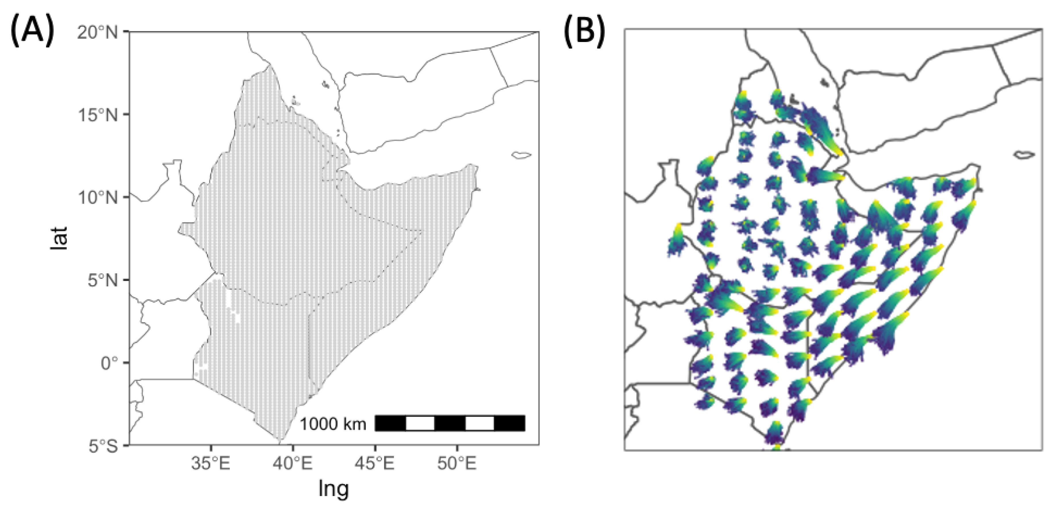
25]. NAME wind trajectories were calculated starting from 3860 source locations spaced on a regular 20km × 20km grid across Ethiopia, Somalia, Eritrea and Kenya (
Figure 1(A)). For a given date and location source, 1000 individual trajectories were calculated, each commencing 2h after local sunrise and terminating 1h before local sunset (
Figure 1(B)). There is stochastic variation in the direction of individual realisations starting from the same location, due to the turbulent nature of the atmosphere as represented in NAME. We calculated the angle for each trajectory between a vector corresponding to the East direction and a vector connecting the start and end location of a trajectory for a specified time.
2.4. Bayesian Inference
2.4.1. Importance Sampling (IS)
Importance sampling is based on using weighted samples from a proposal distribution [
26]. The corresponding importance weights for a sampled set of parameters
can be calculated as:
where
is the target density function (i.e. the von Mises distribution function) and
is the proposal density function.
2.4.2. Effective Sample Size (ESS)
We use Kish’s effective sample size [
27] as a measure of the quality of the posterior distribution. We denote the
ESS for dataset
i after iteration
l as,
Here
is a normalised weight, so that
.
2.4.3. Adaptive Multiple Importance Sampling (AMIS)
The Adaptive Multiple Importance Sampling algorithm (AMIS) is a technique that recycles samples from all previous iterations when constructing a proposal distribution or calculating weights [
28]. For each iteration
, we sample
parameter sets. The corresponding importance weights for a sampled set of parameters
can be calculated as:
where
is a proposal distribution at iteration
l.
For the AMIS algorithm, we set a required ESS for all of the pixels, denoted by . We call datasets ’active’ if they have an ESS below the target, and use the weights for the active datasets to design the proposal for the next iteration of the AMIS algorithm. This targets sampling towards areas of the parameter space that benefit datasets that have not yet reached the required ESS. At iterations , we use the mean weight over the active dataset to determine the next proposal distribution. A suitable proposal can be found by fitting a mixture of Student’s t-distributions to the weighted samples , for . The algorithm continues until all datasets meet the ESS requirement or the maximum number of iterations, I, has been completed.
3. Results
3.1. Illustrative Simulations
3.1.1. Parameter Estimation Using Importance Sampling for a Single Dataset
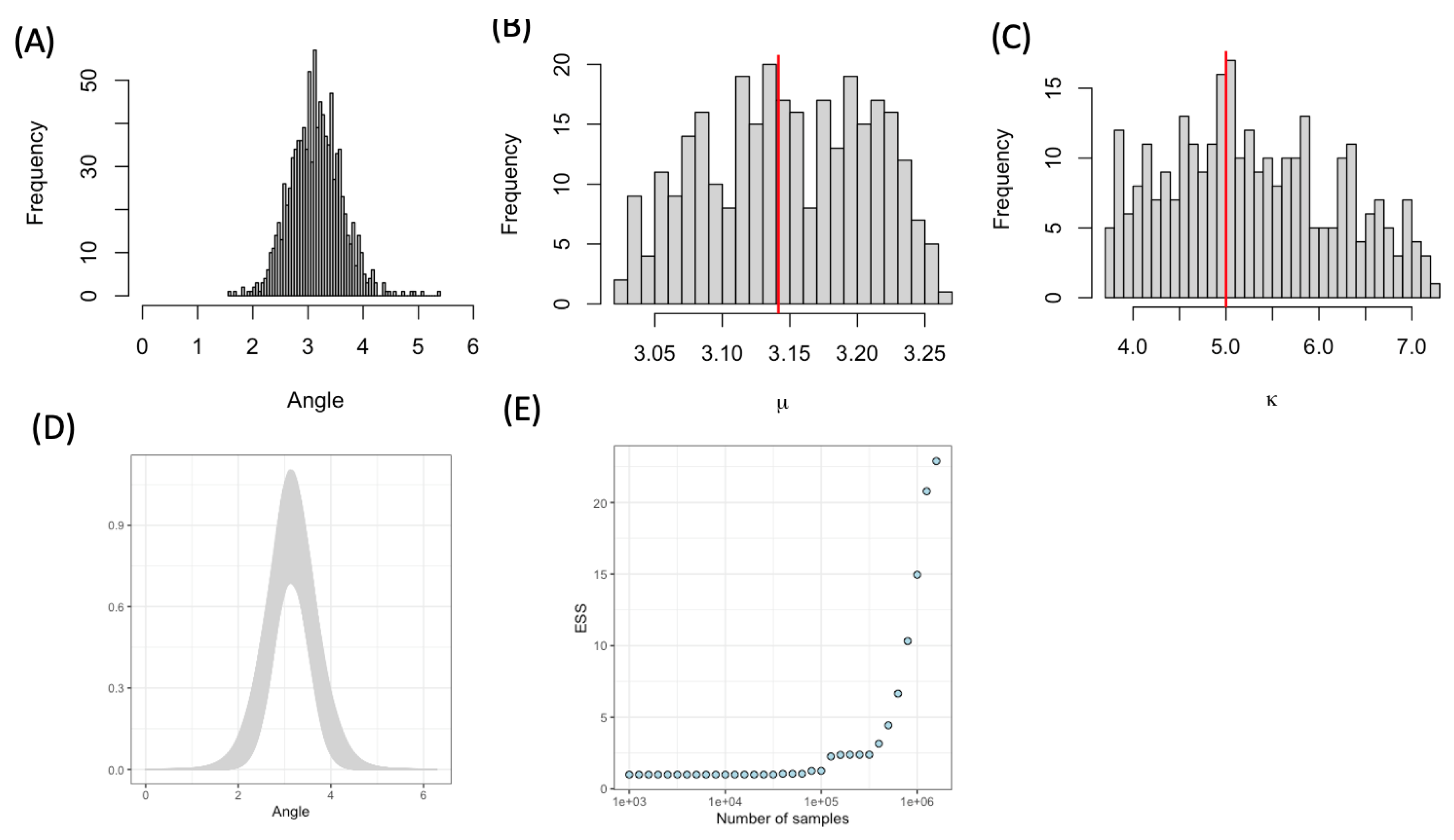
First, we sampled 1000 angles using parameter values
and
(
Figure 2(A)). For the IS, we chose a uniform distribution function as our proposal:
. We varied the number of parameters sets sampled from the proposal from
to
and calculated the effective sample size (ESS) as a function of the number of parameter sets sampled Importance sampling produced a reasonable posterior distribution that recovered the original parameter values (
Figure 2(B)-(C)) and provided a corresponding fit of the von Mises distribution function to the original (
Figure 2(D)). Although the ESS increased with sample size, the ESS was >25 for
samples for this single dataset (
Figure 2(E)).
3.1.2. Parameter Estimation Using AMIS for Multiple Datasets
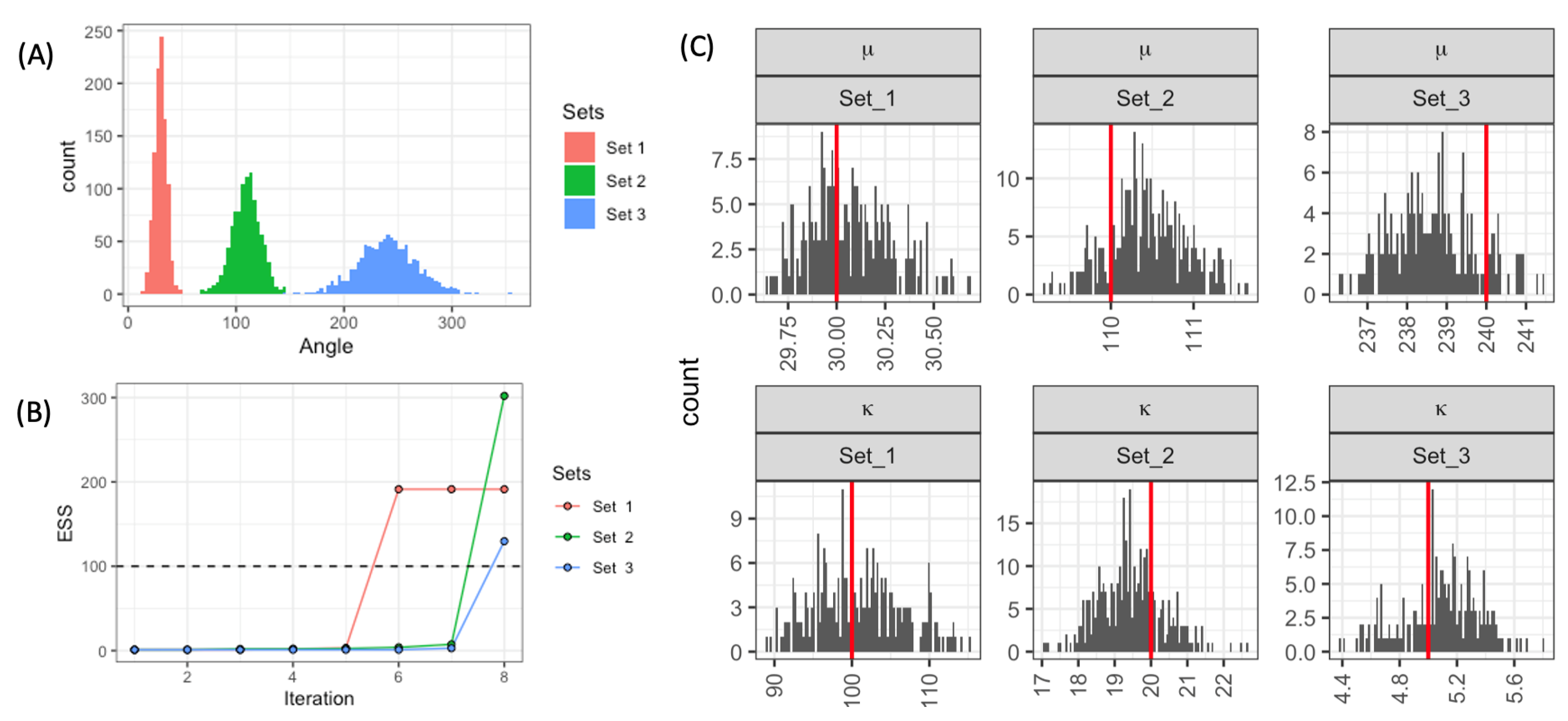
Next, we considered three datasets with differing means and variances. We sampled 1000 angles with the following values of parameters: set 1
; set 2
; and set 3
(
Figure 3(A)). We chose these parameters to produce angle distributions which do not overlap, as well as having different dispersion around their mean. For this case study, we have fitted parameters for the three sets simultaneously using the AMIS algorithm. As in the previous example, we chose a uniform distribution function as our proposal:
. We set the required effective sample size
and we sampled 1000 parameter sets each iteration. The algorithm stopped when all datasets had
. The first dataset reached the required ESS after 6000 sampled parameter sets (
Figure 3(B)). The other two datasets reached the required ESS after 8000 parameter sets to achieve the required
. The posterior distributions recovered the original parameters (
Figure 3(C)).
3.2. Application to NAME Wind Trajectories
Finally, we simultaneously fitted the von Mises distributions to the NAME wind trajectories. We chose three dates: 15 January 2020, 15 August 2020 and 15 January 2021. This resulted in the estimation of parameters for 11,580 datasets, corresponding to 3 x 3860 datasets on the 20km × 20km grid. We chose a uniform distribution function as our proposal:
. We set the required effective sample size
and we sampled 1000 parameter sets each iteration. It took about
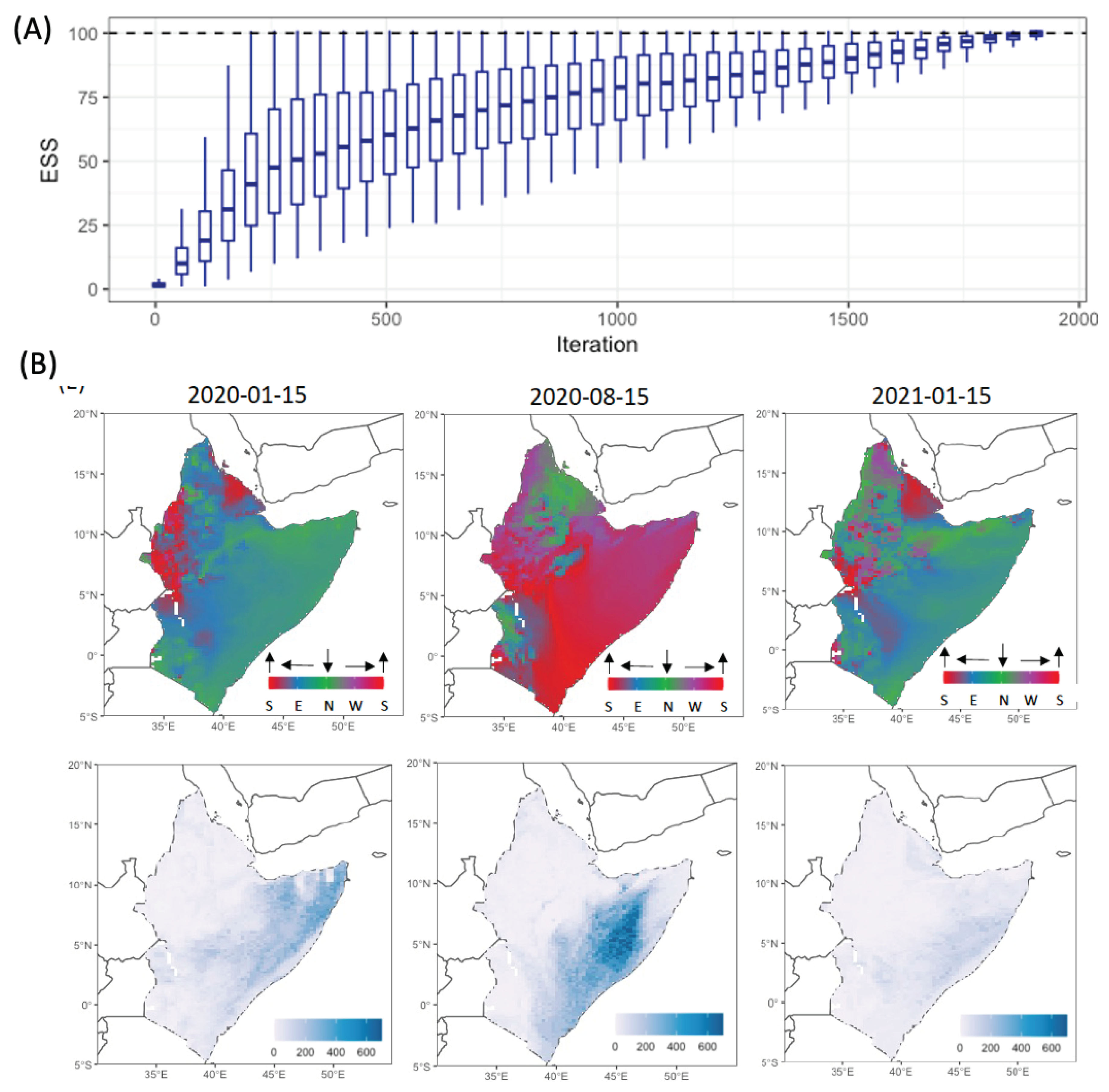
sampled parameters for all datasets to reach the required ESS (
Figure 4(A)). For each grid cell and the three days we provide 100 parameter sets sampled from the posterior distributions in the supplementary materials.
To illustrate global wind trends, we have drawn a single parameter sample from the posterior distribution for each of the 3860 sites and plotted the spatial distribution of these parameters (
Figure 4(B)) for each of the three selected dates. The directional mean for January had similar trends for both 2020 and 2021, i.e. most of wind trajectories had southwards orientations, but some differences in direction could be seen for small areas. The concentration values showed more variation, with northerly wind concentrated less in 2021 than in 2020. Meanwhile, wind trajectories were directed towards the north on 15 August 2020, with a larger range of concentrations in comparison with wind trajectories in January for both 2020 and 2021.
4. Discussion
In situations when the number of datasets is large, performing Bayesian inference can be time consuming. Here we have investigated how adaptive multiple importance sampling can be used to effectively estimate parameters for multiple datasets. As an illustration of the methodology, we fitted the von Mises distribution to wind direction data. For a comparison, we used importance sampling to fit parameters to a single wind angle distribution using synthetic data. Inference using importance sampling recovered the parameter values and captured the original distribution for wind trajectories, but it was prohibitively slow and computationally inefficient ( parameter sets to achieve ESS=25). We showed that AMIS significantly reduced computational effort while maintaining the quality of inference (8000 parameter sets to achieve ESS=100) for three independent datasets. Finally, our results showed that AMIS was able to achieve ESS=100 for >11,000 location and date specific parameters for the NAME wind trajectories with similar computational requirements as a single dataset fitted using importance sampling ( parameter sets).
The migration pathways achieved by flying insects are highly dependent on the seasonal variation of wind patterns [
29,
30,
31]. For example, swarms follow seasonal shifts of the Intertropical Convergence Zone (ITCZ), which can take them to areas of rainfall [
32,
33,
34,
35,
36]. We fitted the von Mises distribution to NAME wind trajectories at two different seasons (January and August). Our analysis confirmed the influence of the ITCZ on local wind trajectories, i.e. southwards orientation in January and northwards orientation in August. Certain areas tended to have a smaller concentration in the direction of wind trajectories, and hence greater variability which is important to account for when predicting long-distance windborne dispersal. Another application of fitting the von Mises distribution to NAME wind data is to compare annual differences in wind behaviour at high resolution, as illustrated in
Figure 4(B).
As the amount of data continues to increase at an exponential rate [
37] and more multi-set data become available, it will be crucial to have computationally efficient methods for parameter estimation. Our proposed methodology can be easily applied to any type of a problem where the target distribution can be formulated due to the universal way the proposal density function is constructed at each iteration. Further research is required to guide the optimal choice of ESS and number of sampled parameters at each iteration for a particular type and size of datasets.
Author Contributions
Conceptualization, R.R., W.T. and C.A.G.; methodology, R.R. and W.T.; software, R.R.; validation, R.R.; formal analysis, R.R.; investigation, R.R.; resources, C.A.G..; data curation, R.R..; writing—original draft preparation, R.R., W.T. and C.A.G.; writing—review and editing, R.R., W.T. and C.A.G.; visualization, R.R.; project administration, C.A.G..; funding acquisition, C.A.G.. All authors have read and agreed to the published version of the manuscript.
Funding
This research was funded by The UK Foreign, Commonwealth and Development Office. C.A.G. also acknowledges support from the Bill and Melinda Gates Foundation.
Data Availability Statement
Analysis code used in this study can be accessed at the following URL: TBA (permanent DOI: zenodo).
References
- Zhang, N.; Berman, S.R.; Joubert, D.; Vialet-Chabrand, S.; Marcelis, L.F.M.; Kaiser, E. Variation of photosynthetic induction in major horticultural crops is mostly driven by differences in stomatal traits. Frontiers in Plant Science 2022, 13. [Google Scholar] [CrossRef] [PubMed]
- Tognetti, M.; Gabor, A.; Yang, M.; Cappelletti, V.; Windhager, J.; Rueda, O.M.; Charmpi, K.; Esmaeilishirazifard, E.; Bruna, A.; de Souza, N.; et al. Deciphering the signaling network of breast cancer improves drug sensitivity prediction. Cell Systems 2021, 12, 401–418. [Google Scholar] [CrossRef] [PubMed]
- Reeves, D.B.; Rolland, M.; Dearlove, B.L.; Li, Y.; Robb, M.L.; Schiffer, J.T.; Gilbert, P.; Cardozo-Ojeda, E.F.; Mayer, B.T. Timing HIV infection with a simple and accurate population viral dynamics model. Journal of The Royal Society Interface 2021, 18, 20210314. [Google Scholar] [CrossRef] [PubMed]
- Padmanabhan, P.; Desikan, R.; Dixit, N.M. Modeling how antibody responses may determine the efficacy of COVID-19 vaccines. Nature Computational Science 2022, 2, 123–131. [Google Scholar] [CrossRef]
- Crump, R.E.; Huang, C.I.; Knock, E.S.; Spencer, S.E.F.; Brown, P.E.; Mwamba Miaka, E.; Shampa, C.; Keeling, M.J.; Rock, K.S. Quantifying epidemiological drivers of gambiense human African Trypanosomiasis across the Democratic Republic of Congo. PLOS Computational Biology 2021, 17, e1008532. [Google Scholar] [CrossRef] [PubMed]
- Akanbi, O.D.; Bhuvanagiri, D.C.; Barcelos, E.I.; Nihar, A.; Gonzalez Hernandez, B.; Yarus, J.M.; French, R.H. Integrating multiscale geospatial analysis for monitoring crop growth, nutrient distribution, and hydrological dynamics in large-scale agricultural systems. Journal of Geovisualization and Spatial Analysis 2024, 8. [Google Scholar] [CrossRef]
- Bhatt, S.; Weiss, D.J.; Cameron, E.; Bisanzio, D.; Mappin, B.; Dalrymple, U.; Battle, K.E.; Moyes, C.L.; Henry, A.; Eckhoff, P.A.; et al. The effect of malaria control on Plasmodium falciparum in Africa between 2000 and 2015. Nature 2015, 526, 207–211. [Google Scholar] [CrossRef] [PubMed]
- Retkute, R.; Touloupou, P.; Basáñez, M.G.; Hollingsworth, T.D.; Spencer, S.E.F. Integrating geostatistical maps and infectious disease transmission models using adaptive multiple importance sampling. The Annals of Applied Statistics 2021, 15. [Google Scholar] [CrossRef]
- Touloupou, P.; Retkute, R.; Hollingsworth, T.D.; Spencer, S.E. Statistical methods for linking geostatistical maps and transmission models: Application to lymphatic filariasis in East Africa. Spatial and Spatio-temporal Epidemiology 2022, 41, 100391. [Google Scholar] [CrossRef] [PubMed]
- Romero-Severson, E.O.; Hengartner, N.; Meadors, G.; Ke, R. Change in global transmission rates of COVID-19 through May 6 2020. PLOS ONE 2020, 15, e0236776. [Google Scholar] [CrossRef]
- Huang, J.; Gómez-Dans, J.L.; Huang, H.; Ma, H.; Wu, Q.; Lewis, P.E.; Liang, S.; Chen, Z.; Xue, J.H.; Wu, Y.; et al. Assimilation of remote sensing into crop growth models: Current status and perspectives. Agricultural and Forest Meteorology 2019, 276–277, 107609. [Google Scholar] [CrossRef]
- Metropolis, N.; Ulam, S. The Monte Carlo method. Journal of the American Statistical Association 1949, 44, 335–341. [Google Scholar] [CrossRef] [PubMed]
- Kahn, H.; Harris, T.E. Estimation of particle transmission by random sampling. National Bureau of Standards applied mathematics series 1951, 12, 27–30. [Google Scholar]
- Burgess, A.J.; Retkute, R.; Murchie, E.H. Photoacclimation and entrainment of photosynthesis by fluctuating light varies according to genotype in Arabidopsis thaliana. Frontiers in Plant Science 2023, 14. [Google Scholar] [CrossRef]
- Prusokiene, A.; Prusokas, A.; Retkute, R. Machine learning based lineage tree reconstruction improved with knowledge of higher level relationships between cells and genomic barcodes. NAR Genomics and Bioinformatics 2023, 5. [Google Scholar] [CrossRef] [PubMed]
- Mardia, K.V. Statistics of directional data. Journal of the Royal Statistical Society: Series B (Methodological) 1975, 37, 349–371. [Google Scholar] [CrossRef]
- Carta, J.A.; Bueno, C.; Ramírez, P. Statistical modelling of directional wind speeds using mixtures of von Mises distributions: Case study. Energy Conversion and Management 2008, 49, 897–907. [Google Scholar] [CrossRef]
- Meyer, M.; Cox, J.A.; Hitchings, M.D.T.; Burgin, L.; Hort, M.C.; Hodson, D.P.; Gilligan, C.A. Quantifying airborne dispersal routes of pathogens over continents to safeguard global wheat supply. Nature Plants 2017, 3, 780–786. [Google Scholar] [CrossRef] [PubMed]
- Meyer, M.; Thurston, W.; Smith, J.W.; Schumacher, A.; Millington, S.C.; Hodson, D.P.; Cressman, K.; Gilligan, C.A. Three-Dimensional Visualization of long-range atmospheric transport of crop pathogens and insect pests. Atmosphere 2023, 14, 910. [Google Scholar] [CrossRef]
- Jones, A.; Thomson, D.; Hort, M.; Devenish, B. The U.K. Met Office’s next-generation atmospheric dispersion model, NAME III. In Air pollution modeling and its application XVII; Springer US, 2007; pp. 580–589. [CrossRef]
- Burgin, L.E.; Gloster, J.; Sanders, C.; Mellor, P.S.; Gubbins, S.; Carpenter, S. Investigating incursions of bluetongue virus using a model of long-distance culicoides biting midge dispersal. Transboundary and emerging diseases 2012, 60, 263–272. [Google Scholar] [CrossRef]
- Retkute, R.; Hinton, R.G.K.; Cressman, K.; Gilligan, C.A. Regional differences in control operations during the 2019–2021 desert locust upsurge. Agronomy 2021, 11, 2529. [Google Scholar] [CrossRef]
- Mardia, K.V.; Jupp, P.E. Directional statistics; Wiley Series in Probability and Statistics; John Wiley & Sons: Chichester, England, 1999. [Google Scholar]
- Tsagris, M.; Papadakis, M. Taking R to its limits: 70+ tips 2018. [CrossRef]
- Walters, D.; Baran, A.J.; Boutle, I.; Brooks, M.; Earnshaw, P.; Edwards, J.; Furtado, K.; Hill, P.; Lock, A.; Manners, J.; et al. The Met Office unified model global atmosphere 7.0/7.1 and JULES global land 7.0 configurations. Geoscientific Model Development 2019, 12, 1909–1963. [Google Scholar] [CrossRef]
- Ripley, B.D. Stochastic simulation; Wiley, 1987. [CrossRef]
- Kish, L. Survey sampling; John Wiley & Sons: Nashville, TN, 1966. [Google Scholar]
- Cappé, O.; Douc, R.; Guillin, A.; Marin, J.M.; Robert, C.P. Adaptive importance sampling in general mixture classes. Stat. Comput. 2008, 18, 447–459. [Google Scholar] [CrossRef]
- Cheke, R.A.; Tratalos, J.A. Migration, patchiness, and population processes illustrated by two migrant pests. BioScience 2007, 57, 145–154. [Google Scholar] [CrossRef]
- Chapman, J.W.; Nesbit, R.L.; Burgin, L.E.; Reynolds, D.R.; Smith, A.D.; Middleton, D.R.; Hill, J.K. Flight orientation behaviors promote optimal migration trajectories in high-flying insects. Science 2010, 327, 682–685. [Google Scholar] [CrossRef] [PubMed]
- Dingle, H. Migration to special habitats. In Migration; Oxford University Press, 2014; pp. 183–194.
- Rainey, R.C. Weather and the movements of locust swarms: A new hypothesis. Nature 1951, 168, 1057–1060. [Google Scholar] [CrossRef]
- Draper, J. The direction of desert locust migration. The journal of animal ecology 1980, 49, 959. [Google Scholar] [CrossRef]
- Pedgley, D.E. (Ed.) Desert locust forecasting manual; Natural Resources Institute: Chatham, England, 1981. [Google Scholar]
- Homberg, U. Sky compass orientation in desert locusts—Evidence from field and laboratory studies. Frontiers in behavioral neuroscience 2015, 9. [Google Scholar] [CrossRef] [PubMed]
- Homberg, U.; Hensgen, R.; Jahn, S.; Pegel, U.; Takahashi, N.; Zittrell, F.; Pfeiffer, K. The sky compass network in the brain of the desert locust. Journal of Comparative Physiology A 2022. [Google Scholar] [CrossRef]
- Hashem, I.A.T.; Yaqoob, I.; Anuar, N.B.; Mokhtar, S.; Gani, A.; Ullah Khan, S. The rise of “big data” on cloud computing: Review and open research issues. Information Systems 2015, 47, 98–115. [Google Scholar] [CrossRef]
|
Disclaimer/Publisher’s Note: The statements, opinions and data contained in all publications are solely those of the individual author(s) and contributor(s) and not of MDPI and/or the editor(s). MDPI and/or the editor(s) disclaim responsibility for any injury to people or property resulting from any ideas, methods, instructions or products referred to in the content. |
© 2024 by the authors. Licensee MDPI, Basel, Switzerland. This article is an open access article distributed under the terms and conditions of the Creative Commons Attribution (CC BY) license (https://creativecommons.org/licenses/by/4.0/).


