Submitted:
02 April 2024
Posted:
02 April 2024
You are already at the latest version
Abstract
Keywords:
1. Introduction
- Presents the novel of the forecasting formulation model for the ICPT regime in Malaysia where the accuracy of the model has configured and tested with time series and machine learning techniques.
- Provides comprehensive analysis of the data collected from the real generation system while putting much widespread discussion on the three-baseline model for the ICPT main component.
- Contributes to provide valuable forecasting ICPT price information for the electricity consumers in Peninsular Malaysia where the sustainable electricity market can be enhanced significantly.
2. Related Previous Work of Forecasting Model
3. Formulation of ICPT
4. Methodology
4.1. Forecasting Formulation
- (1)
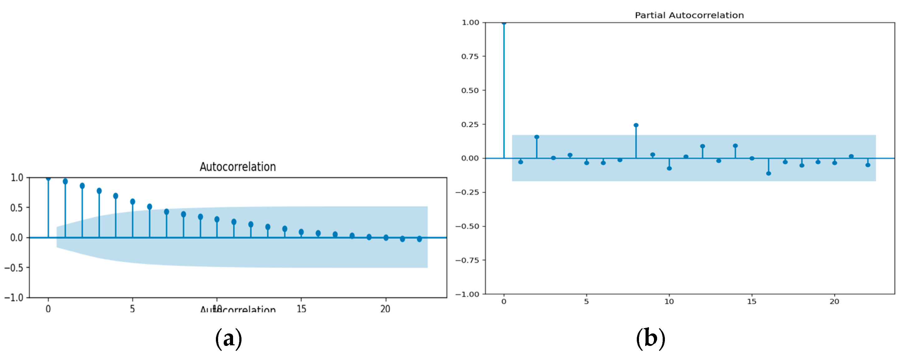
- Auto Regression (AR): Regression analysis is used to compare the time series to its prior values, such as y(t-1), y(t-2) etc. The letter p stands for the lag order.
- (2)
- Integration (I): Differencing is used to make the time series stationary. The difference's order is indicated by the letter d.
- (3)
- Moving Average (MA): Regression is performed on the time series using residuals from previous observations, such as error ε(t-1), error ε(t-2) etc. The error lag order is indicated by the letter q. In the equation above, y^' is the differenced series, ϕ1 is the first AR term's coefficient, p is the AR term's order, θ11 is the first MA term's coefficient, q is the MA term's order, and εt is the error.
4.2. Data Set Collection
4.3. Implementation of Techniques
- 1)
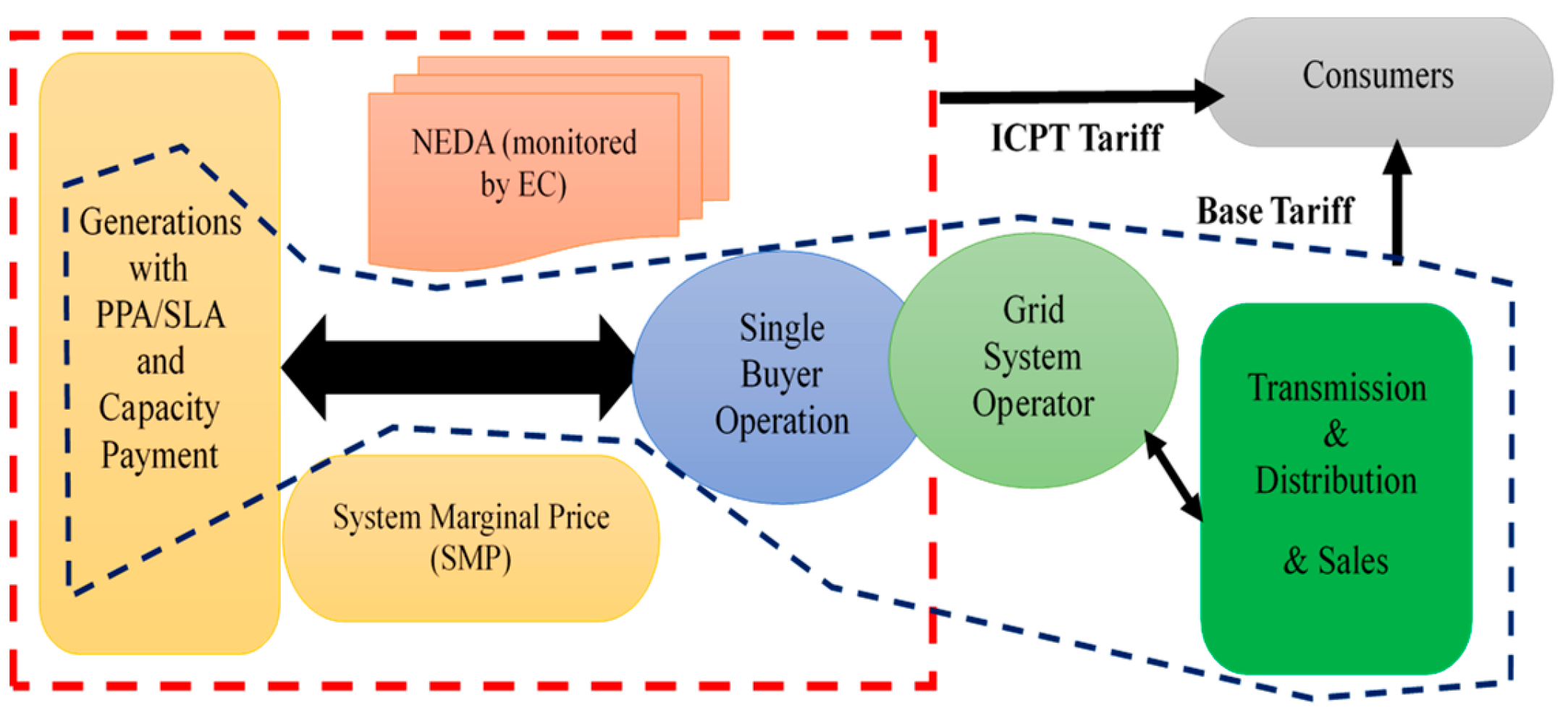
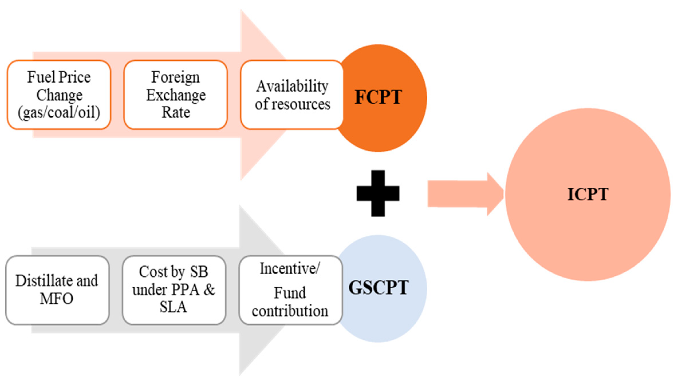
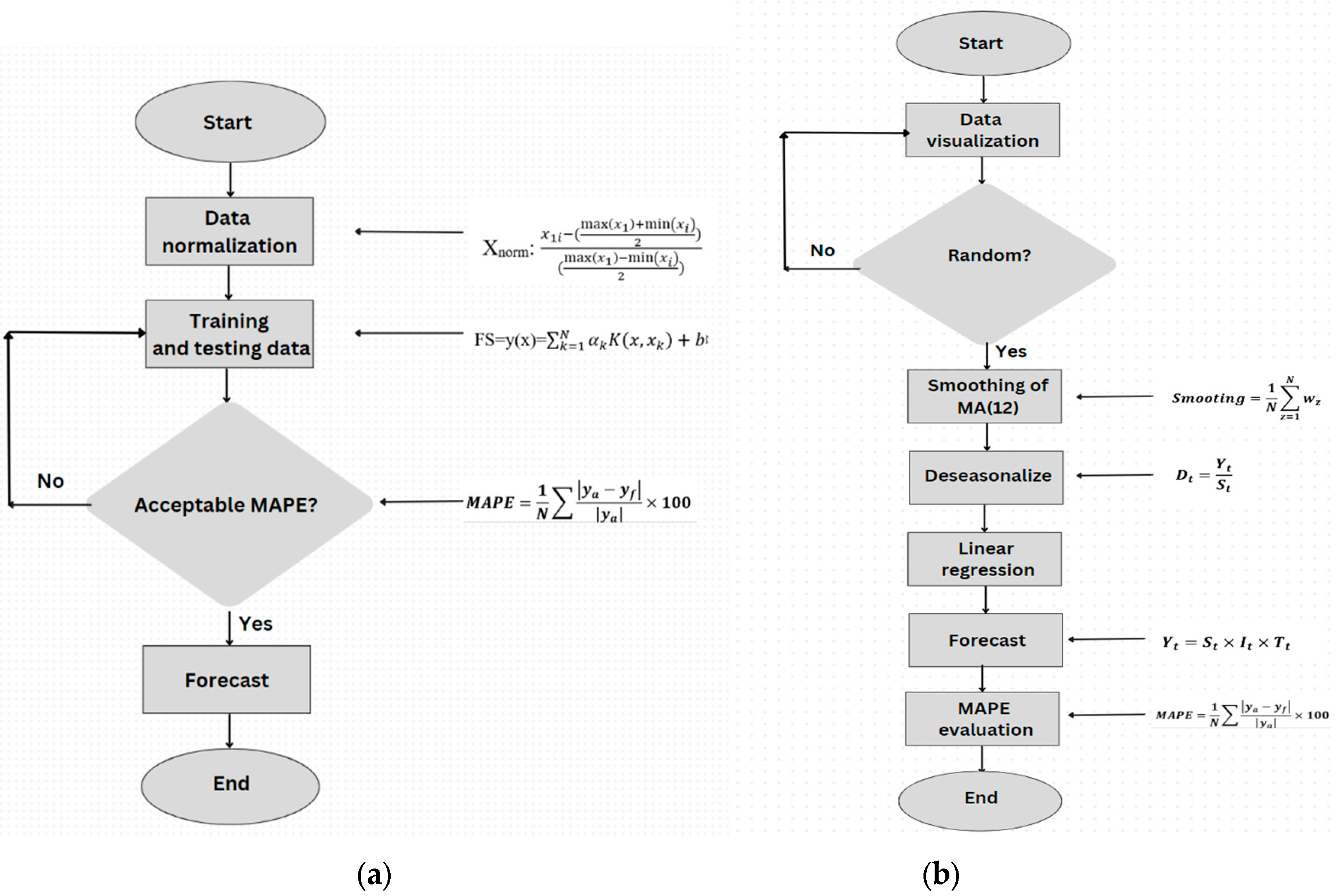
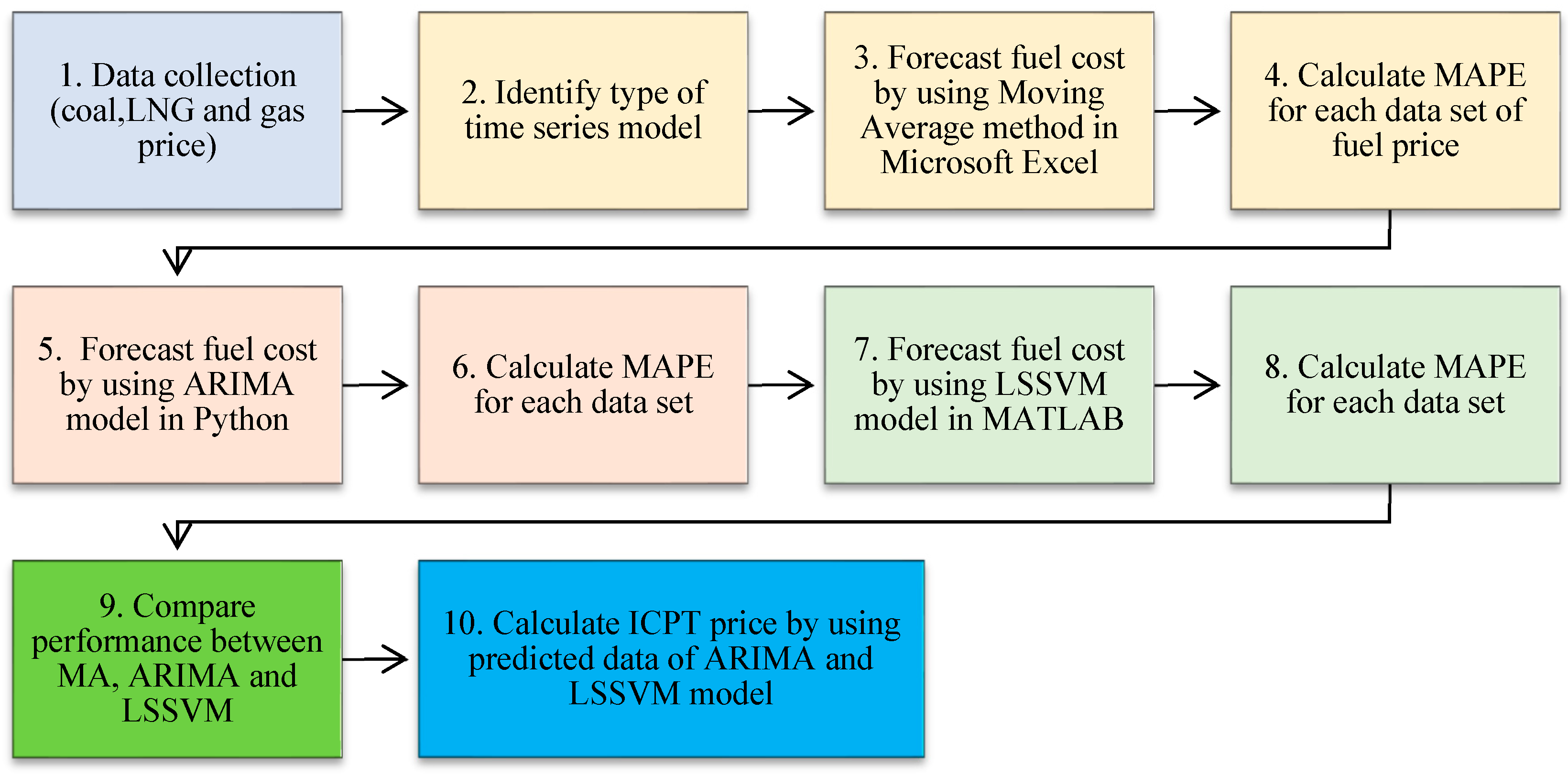
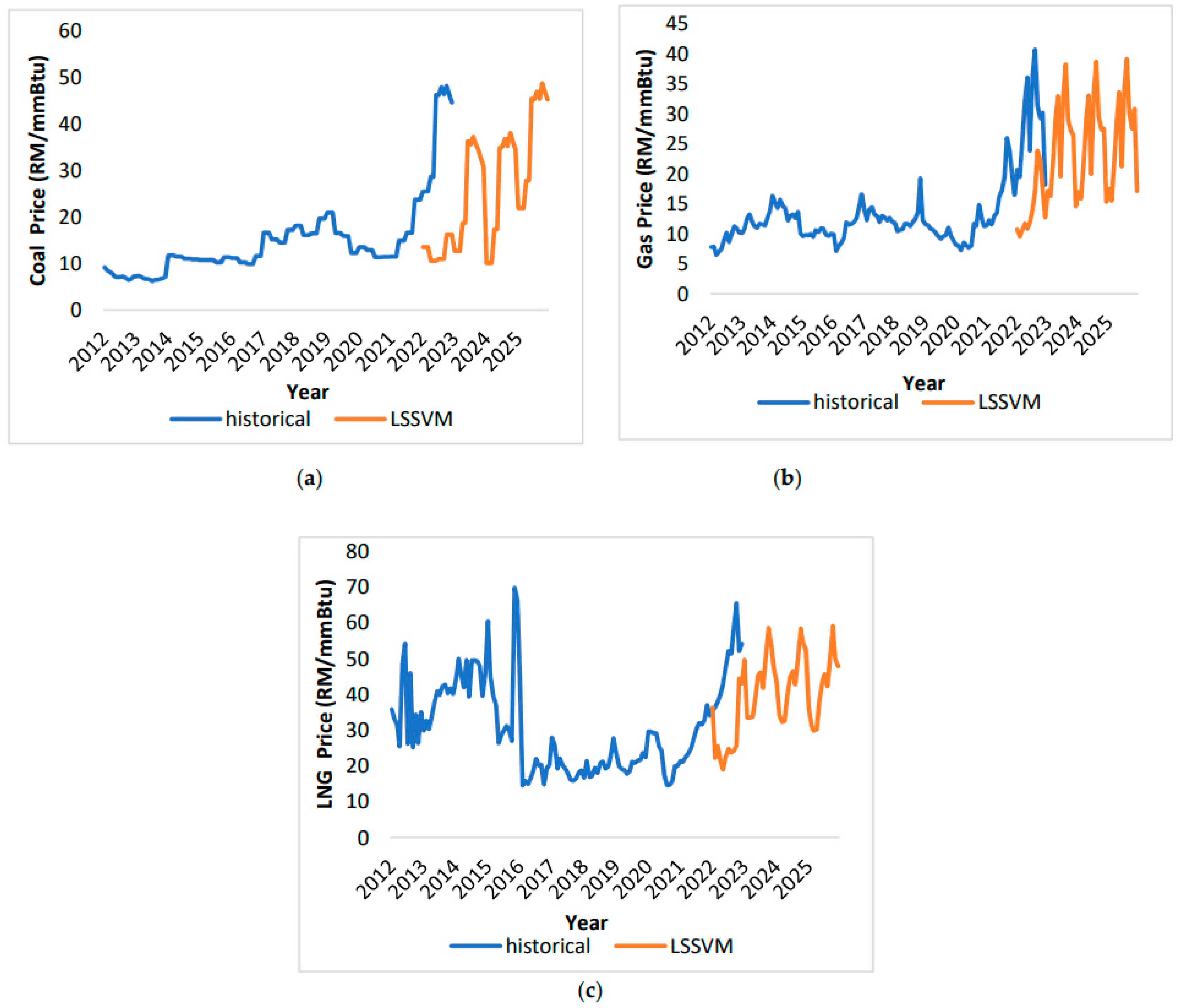
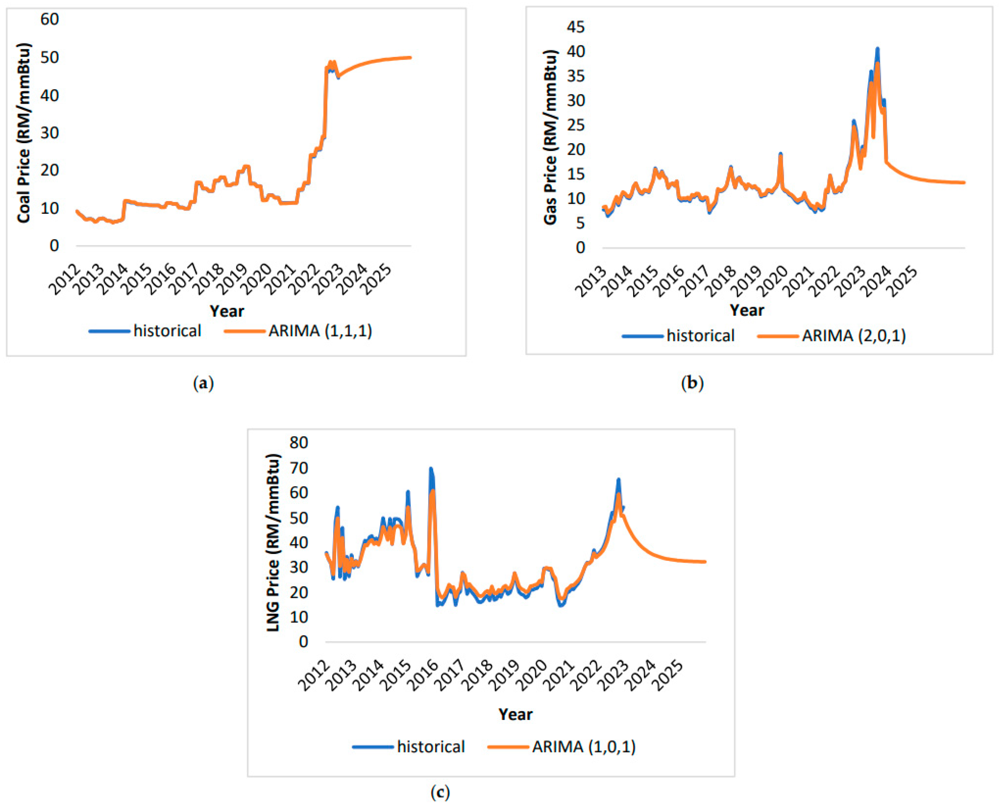
- The initial step in calculating ICPT involves determining the interim fuel cost pass through adjustment for a six-month period (IFUCS) using Equation (6). The estimated and actual total fuel costs (Cm, Dm) were derived from the projected fuel cost using the ARIMA and LSSVM models. The data for Dm was not accessible due to limited resources. As a result, forecasted data was utilised instead. The estimated total qualifying sales (Fm) were acquired from websites of Single Buyers (SB). The audited total qualifying sales, to which the ICPT adjustment is applied, was obtained from the Grid System Operator (GSO) website. By using Equation (5), the average fuel cost for was calculated. The total forecasted fuel cost (FFULs) for six months is derived from the previously forecasted fuel cost. The weighted average cost of capital of Regulatory Period 3 (RP3) is set by the government at 7.3%. The forecasted total electricity sales in year 2021 as made at the time of setting the Base Average Tariff was obtained from SB.
- 2)
- Then, using Equation (6), the first fuel cost pass-through adjustment (As) was determined.
- 3)
- Next, Equation (7) was used to determine the interim other generation cost pass-through adjustment (IGSCs). System marginal pricing (SMP) at SB websites was used to determine the estimated and actual total other generation cost (Gm, Hm).
- 4)
- To determine the average other generation cost (AGSCs) using Equation (8), the forecasted other generation cost is obtained by subtracting the generation margin (Gm) from the forecasted fuel and fuel-related costs (FFULs).
- 5)
- Equation (7) is then used to compute the first other generation cost pass-through adjustment (Bs) in the six-month period.
- 6)
- The next part involves calculating the secondary fuel and additional generation cost pass-through adjustment within the designated six-month timeframe. This can be achieved by utilising Equation (10)-(11).
- 7)
- The remuneration rates for ICPT adjustment, specifically IARRs-1 and IARRs-2, are constantly set at 2.8738 and 2.86, respectively.
- 8)
- The six-month generation cost adjustment was determined using Equation (3).
- 9)
- Equation (12) was used to compute the fund contribution (FUNDs). The approved payment (FUNPm) from the Electricity Industry Fund (EIF) and the payment by the Single Buyer (FUNTm) into the EIF are fixed at MYR 1.6 billion and MYR 1.3 billion, respectively.
- 10)
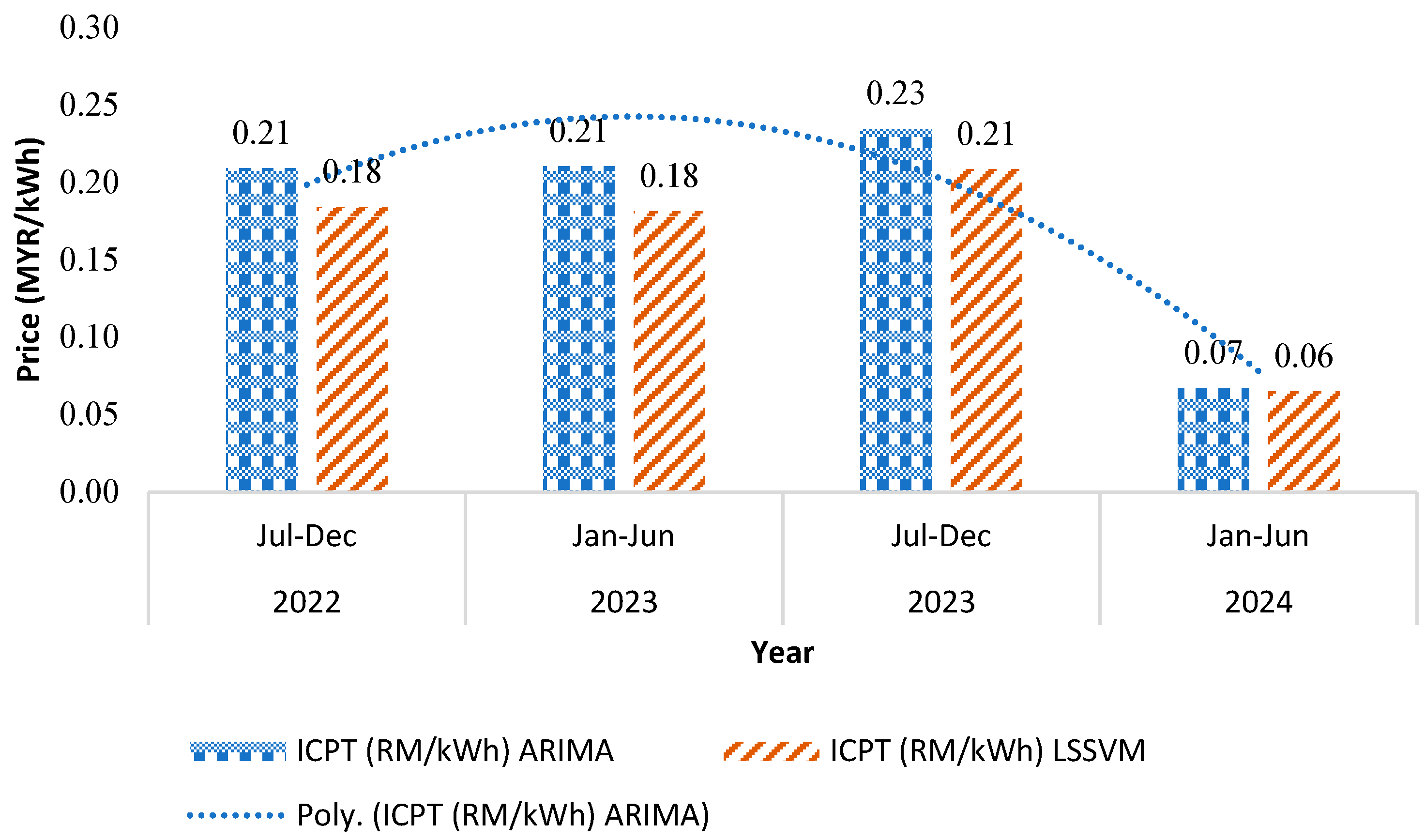
- The ICPT price was then determined using Equation (2).
5. Results and Discussion
5.1. Moving Average (MA) Forecasting Profile
5.2. LSSVM Forecasting Profile
5.3. ARIMA Forecasting Profile
5.4. Analysis of the MAPE
5.5. Discussion of the Forecast ICPT
6. Conclusion
Author Contributions
Funding
Acknowledgments
Conflicts of Interest
References
- Y. Chen, M. Li, Y. Yang, C. Li, Y. Li, and L. Li, “A hybrid model for electricity price forecasting based on least square support vector machines with combined kernel,” Journal of Renewable and Sustainable Energy, vol. 10, no. 5, 2018. [CrossRef]
- M. Sibeperegasam, V. K. Ramachandaramurthy, F. Li, and S. Walker, “De-Regulation of Electricity Industry: A Malaysian Perspective,” International Journal of Electronics and Electrical Engineering, vol. 8, no. 2, pp. 17–23, 2020. [CrossRef]
- M. F. Sulaima, S. A. A. Hanipah, N. R. A. Razif, I. A. W. A. Razak, A. F. A. Kadir, and Z. H. Bohari, “Industrial Energy Load Profile Forecasting under Enhanced Time of Use Tariff (ETOU) using Artificial Neural Network,” International Journal of Advanced Computer Science and Applications, vol. 11, no. 12, pp. 204–209, 2020. [CrossRef]
- N. Z. Z. Abidin and J. B. Ibrahim, “Embracing renewables - Overcoming integration challenges from Malaysia’s utility perspective,” 2015 IEEE Eindhoven PowerTech, PowerTech 2015, 2015. [CrossRef]
- M. Sibeperegasam, V. K. Ramachandaramurthy, S. Walker, and J. Kanesan, “Malaysia’s electricity market structure in transition,” Utilities Policy, vol. 72, no. July, p. 101266, 2021. [CrossRef]
- C. Kuster, Y. Rezgui, and M. Mourshed, “Electrical load forecasting models: A critical systematic review,” Sustainable Cities and Society, vol. 35, no. June, pp. 257–270, 2017. [CrossRef]
- M. Imani and H. Ghassemian, “Electrical Load Forecasting Using Customers Clustering and Smart Meters in Internet of Things,” 9th International Symposium on Telecommunication: With Emphasis on Information and Communication Technology, IST 2018, pp. 113–117, 2019. [CrossRef]
- J. Aguilar, A. Garces-jimenez, M. D. R-moreno, and R. García, “A systematic literature review on the use of artificial intelligence in energy self-management in smart buildings,” Renewable and Sustainable Energy Reviews, vol. 151, no. May, p. 111530, 2021. [CrossRef]
- R. Porteiro and S. Nesmachnow, “Forecasting hourly electricity demand of Uruguay for the next day using artificial neural networks,” 2020 IEEE PES Transmission and Distribution Conference and Exhibition - Latin America, T and D LA 2020, pp. 8–13, 2020. [CrossRef]
- T. N. B. TNB, “Integrated Annual Report 2020,” Annual Report 2020, p. 360, 2020.
- N. Singh and S. R. Mohanty, “A Review of Price Forecasting Problem and Techniques in Deregulated Electricity Markets,” Journal of Power and Energy Engineering, vol. 03, no. 09, pp. 1–19, 2015. [CrossRef]
- P. Hendikawati, Subanar, Abdurakhman, and Tarno, “A survey of time series forecasting from stochastic method to soft computing,” Journal of Physics: Conference Series, vol. 1613, no. 1, 2020. [CrossRef]
- Cruz A., A. Muñoz, J. L. Zamora, and R. Espínola, “The effect of wind generation and weekday on Spanish electricity spot price forecasting,” Electric Power Systems Research, vol. 81, no. 10, pp. 1924–1935, 2011. [CrossRef]
- G. Gao, K. Lo, and F. Fan, “Comparison of ARIMA and ANN Models Used in Electricity Price Forecasting for Power Market,” Energy and Power Engineering, vol. 09, no. 04, pp. 120–126, 2017. [CrossRef]
- E. Almeshaiei and H. Soltan, “A methodology for Electric Power Load Forecasting,” Alexandria Engineering Journal, vol. 50, no. 2, pp. 137–144, 2011. [CrossRef]
- Abedinia O., N. Amjady, and H. Zareipour, “A New Feature Selection Technique for Load and Price Forecast of Electrical Power Systems,” IEEE Transactions on Power Systems, vol. 32, no. 1, pp. 62–74, 2017. [CrossRef]
- T. J. Sturgeon, “Proceedings 59th ISI World Statistics Congress, 25-30 August 2013, Hong Kong (Session STS024) p.1550,” no. August, pp. 25–30, 2013.
- V. E. Ali Azadeh, Mohsen Moghaddam, Mehdi Khakzad, “54. A flexible neural network-fuzzy mathematical programming algorithm for improvement of oil price estimation and forecasting _ Elsevier Enhanced Reader.pdf.”.
- J. Mei, D. He, R. Harley, T. Habetler, and G. Qu, “A random forest method for real-time price forecasting in New York electricity market,” IEEE Power and Energy Society General Meeting, vol. 2014-October, no. October, 2014. [CrossRef]
- Z. Mustaffa, M. H. Sulaiman, and M. N. M. Kahar, “Training LSSVM with GWO for price forecasting,” 2015 4th International Conference on Informatics, Electronics and Vision, ICIEV 2015, pp. 1–6, 2015. [CrossRef]
- J. Zhang, Z. Tan, and S. Yang, “Day-ahead electricity price forecasting by a new hybrid method,” Computers and Industrial Engineering, vol. 63, no. 3, pp. 695–701, 2012. [CrossRef]
- L. Z. Li Xie, Hua Zheng, “Electricity Price Forecasting by Clustering-LSSVM,” pp. 697–702, 2007.
- Q. Ge et al., “Industrial Power Load Forecasting Method Based on Reinforcement Learning and PSO-LSSVM,” IEEE Transactions on Cybernetics, vol. 52, no. 2, pp. 1112–1124, 2022. [CrossRef]
- Emhamed A. A. and J. Shrivastava, “Electrical load distribution forecasting utilizing support vector model (SVM),” Materials Today: Proceedings, vol. 47, pp. 41–46, 2021. [CrossRef]
- Ali A. N. F., M. F. Sulaima, I. A. W. A. Razak, A. F. A. Kadir, and H. Mokhlis, “Artificial Intelligence Application in Demand Response: Advantages, Issues, Status, and Challenges,” IEEE Access, vol. 11, no. December 2022, pp. 16907–16922, 2023. [CrossRef]
- Z. Mustaffa, Y. Yusof, and S. S. Kamaruddin, “Gasoline Price Forecasting: An Application of LSSVM with Improved ABC,” Procedia - Social and Behavioral Sciences, vol. 129, pp. 601–609, 2014. [CrossRef]
- M. H. L. Lee et al., “A Comparative Study of Forecasting Electricity Consumption Using Machine Learning Models,” Mathematics, vol. 10, no. 8, 2022. [CrossRef]
- G. Bandyopadhyay, “Gold Price Forecasting Using ARIMA Model,” Journal of Advanced Management Science, no. March, pp. 117–121, 2016. [CrossRef]
- S. Singh, K. S. Parmar, S. J. S. Makkhan, J. Kaur, S. Peshoria, and J. Kumar, “Study of ARIMA and least square support vector machine (LS-SVM) models for the prediction of SARS-CoV-2 confirmed cases in the most affected countries,” Chaos, Solitons and Fractals, vol. 139, p. 110086, 2020. [CrossRef]
- “Malaysia Energy Statistics Handbook,” Department of Energy Management and Industrial Development Suruhanjaya Tenaga (Energy Commission), vol. 1, p. 86, 2020.

| Year | Fuel Type | MAPE (%) | |||
|---|---|---|---|---|---|
| MA | ARIMA | LSSVM | |||
| 2022 | Coal | 29.79 | 1.63 | 26.28 | |
| 2022 | Gas | 32.94 | 5.47 | 34.46 | |
| 2022 | LNG | 39.78 | 5.09 | 36.90 | |
Disclaimer/Publisher’s Note: The statements, opinions and data contained in all publications are solely those of the individual author(s) and contributor(s) and not of MDPI and/or the editor(s). MDPI and/or the editor(s) disclaim responsibility for any injury to people or property resulting from any ideas, methods, instructions or products referred to in the content. |
© 2024 by the authors. Licensee MDPI, Basel, Switzerland. This article is an open access article distributed under the terms and conditions of the Creative Commons Attribution (CC BY) license (http://creativecommons.org/licenses/by/4.0/).


