Submitted:
04 April 2024
Posted:
04 April 2024
You are already at the latest version
Abstract
Keywords:
0. Introduction
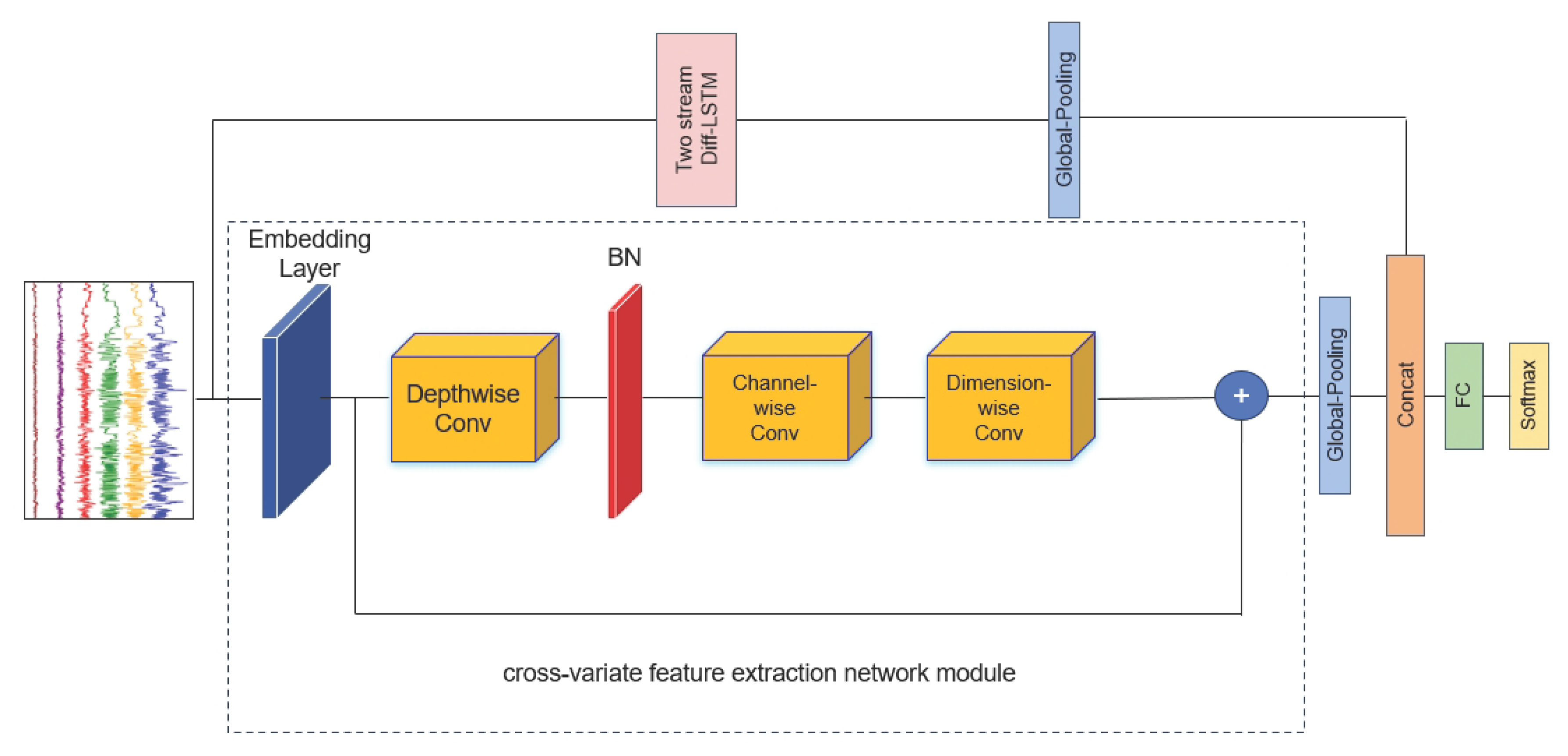
- We propose a novel multivariate time series classification network called Temporal Difference and Cross-variate Fusion Network(TDCFN) to enhance the feature representation capability and improve the classification accuracy of the MTSC task through the combination of two-stream Diff-LSTM and cross-variate feature extraction network, which simultaneously models temporal features and inter-variable features.
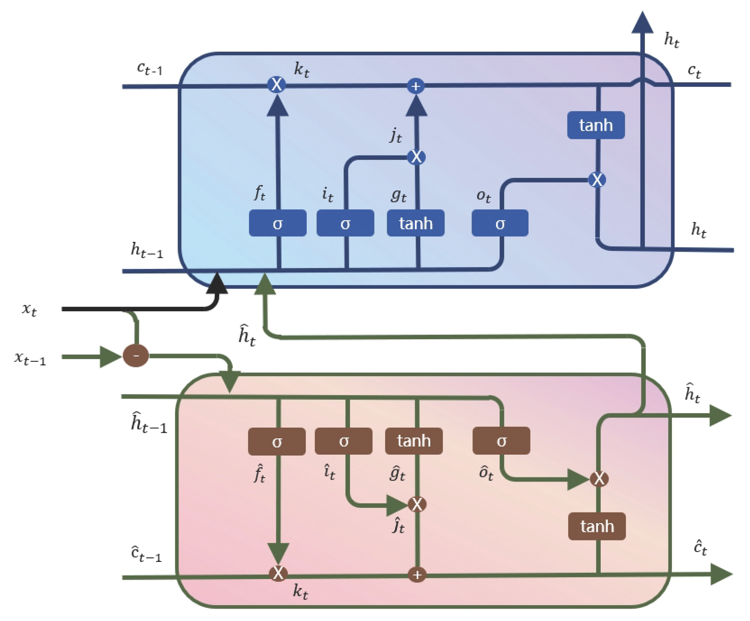
- We obtain the input of LSTM by preprocessing the time series data into differential and source data, with a focus on extracting the temporal features by transforming the LSTM into a two-stream model, which takes advantage of the dynamic evolution of the time series.
- We capture the dependencies between variables and learn the information representation through a cross-variate features extracting network module to generate latent features.
- We perform extensive experiments on MTS benchmark datasets. Experiments on ten benchmark datasets show that TDCFN outperforms state-of-the-art strategies on the MTSC task.
1. Related Works
1.1. Pattern-Based Multivariate Time Series Classification Algorithm
1.2. DL-Based Multivariate Time Series Classification Algorithm
2. Method
2.1. Problem Statement
2.2. Model Architecture Overview
| Algorithm 1:The pseudo-code of TDCFN. |
|
1. Input: A set of Multivariate time series X
2. Output: The probability P of each category
3. Initialize: Parameters of TDCFN
4. Forward Pass:
5. Obtain two levels of temporal feature representations by applying Two Stream Diff-LSTM on X
6. Compute the output using the embedding layer:
7. Compute the cross-variate feature extraction network module output by applying depthwisen, channel-wise and dimension-wise convolutions and skip connection operations:
8. Acquire feature and by global average pooling operation on and respectively
9. Concatenate and and obtain
10. Fed into fully connected layers to obtain the low-dimensional embedding
11. Apply softmax function to obtain the probability distribution P
12. Backward Pass:
13. Compute the loss using the predicted probabilities and the ground truth labels
14. Perform backpropagation to update the parameters of the entire network
|
2.3. Two Stream Diff-LSTM Module
2.4. Cross-Variate Feature Extraction Network Module
2.5. Feature Fusion and Multi-Class Classification Module
3. Experimental Results and Analysis
3.1. Dataset
3.2. Evaluation Metrics
3.3. Experimental Performance
- 1NN-ED and 1NN-ED(norm): These classifiers are traditional distance-based model, which utilize the one-nearest neighbor algorithm with Euclidean distance, both with and without data normalization. The Euclidean distance metric measures the straight-line distance between two points in a multidimensional space. This baseline method is widely used in time series classification tasks due to its simplicity and effectiveness.
- 1NN-DTW-i and 1NN-DTW-i(norm): These classifiers are traditional distance-based model,which employ dimension-independent Dynamic Time Warping (DTW) with and without normalization. The DTW algorithm computes distances based on the sum of DTW distances for each dimension of the time series data. DTW is a flexible and robust measure that accounts for variations in the temporal alignment of sequences, making it suitable for time series classification tasks.
- 1NN-DTW-D and 1NN-DTW-D(norm): These classifiers are traditional distance-based model, which utilize dimension-dependent Dynamic Time Warping (DTW-D) with and without normalization. Unlike the dimension-independent DTW approach, DTW-D directly computes the DTW distance based on multidimensional points, rather than treating each dimension separately. This variant of DTW is particularly useful when the dimensions of the time series data are interdependent and require joint consideration during distance computation.
- WEASEL+MUSE: This framework is feature-based model based on the bag-of-patterns (BOP) approach and represents the latest advancement in multivariate time series classification[16].
- MLSTM-FCN: This algorithm is one of state-of-the-art deep learning based framework designed for multivariate time series classification. The model architecture includes an LSTM layer, stacked CNN layers, and a Squeeze-and-Excitation block for feature extraction. We utilize the source code provided by the authors and execute the approach using default parameter settings, as described in the original work[26].
3.4. Ablation Experiments
- Multilayer Perceptron(MLP) Classifier: In this ablation experiment, we constructed a model comprising solely a fully connected layer classifier, which is also called Multilayer Perceptron(MLP) Classifier, devoid of any additional feature extraction or processing modules. This experiment aims to serve as a baseline comparison to evaluate the significance of the feature extraction components present in the full TDCFN model.
- Without Two Stream Diff-LSTM module: This experiment involved removing the Two Stream Diff-LSTM module, which is responsible for capturing temporal features containing dynamic differential information. By conducting this ablation experiment, we aimed to understand the influence of this module on the overall performance of the model.
- Without Cross-variate feature extraction network module: In this experiment, we excluded the Cross-variate feature extraction network module, which is designed to extract relational features among variables. The purpose was to assess the significance of this module in enhancing the model’s ability to capture inter-variable relationships and representation.
4. Conclusion
References
- Bagnall A, Lines J, Bostrom A, et al. The great time series classification bake off: A review and experimental evaluation of recent algorithmic advances[J]. Data mining and knowledge discovery, 2017, 31: 606-660. [CrossRef]
- Du M, Wei Y, Zheng X, et al. Multi-feature based network for multivariate time series classification[J]. Information Sciences, 2023, 639: 119009. [CrossRef]
- Fan J, Zhang K, Huang Y, et al. Parallel spatio-temporal attention-based TCN for multivariate time series prediction[J]. Neural Computing and Applications, 2023, 35(18): 13109-13118. [CrossRef]
- Singhal A, Seborg D E. Clustering multivariate time-series data[J]. Journal of Chemometrics: A Journal of the Chemometrics Society, 2005, 19(8): 427-438.
- Blázquez-García A, Conde A, Mori U, et al. A review on outlier/anomaly detection in time series data[J]. ACM Computing Surveys (CSUR), 2021, 54(3): 1-33. [CrossRef]
- Qin Z, Zhang Y, Meng S, et al. Imaging and fusing time series for wearable sensor-based human activity recognition[J]. Information Fusion, 2020, 53: 80-87. [CrossRef]
- Yang J, Nguyen M N, San P P, et al. Deep convolutional neural networks on multichannel time series for human activity recognition[C]//Ijcai. 2015, 15: 3995-4001.
- Hasasneh A, Kampel N, Sripad P, et al. Deep learning approach for automatic classification of ocular and cardiac artifacts in meg data[J]. Journal of Engineering, 2018, 2018. [CrossRef]
- Cheng X, Li G, Ellefsen A L, et al. A novel densely connected convolutional neural network for sea-state estimation using ship motion data[J]. IEEE Transactions on Instrumentation and Measurement, 2020, 69(9): 5984-5993. [CrossRef]
- Zhao B, Lu H, Chen S, et al. Convolutional neural networks for time series classification[J]. Journal of Systems Engineering and Electronics, 2017, 28(1): 162-169. [CrossRef]
- Seto S, Zhang W, Zhou Y. Multivariate time series classification using dynamic time warping template selection for human activity recognition[C]//2015 IEEE symposium series on computational intelligence. IEEE, 2015: 1399-1406.
- Abanda A, Mori U, Lozano J A. A review on distance based time series classification[J]. Data Mining and Knowledge Discovery, 2019, 33(2): 378-412. [CrossRef]
- Sharabiani A, Darabi H, Rezaei A, et al. Efficient classification of long time series by 3-d dynamic time warping[J]. IEEE Transactions on Systems, Man, and Cybernetics: Systems, 2017, 47(10): 2688-2703. [CrossRef]
- Chen Y, Hu B, Keogh E, et al. Dtw-d: Time series semi-supervised learning from a single example[C]//Proceedings of the 19th ACM SIGKDD international conference on Knowledge discovery and data mining. 2013: 383-391.
- Rakthanmanon T, Keogh E. Data mining a trillion time series subsequences under dynamic time warping[C]//Twenty-Third International Joint Conference on Artificial Intelligence. 2013.
- Schäfer P, Leser U. Multivariate time series classification with WEASEL+ MUSE[J]. arXiv:1711.11343, 2017.
- Li G, Choi B, Xu J, et al. Shapenet: A shapelet-neural network approach for multivariate time series classification[C]//Proceedings of the AAAI conference on artificial intelligence. 2021, 35(9): 8375-8383.
- Ma Q, Zhuang W, Cottrell G. Triple-shapelet networks for time series classification[C]//2019 IEEE International Conference on Data Mining (ICDM). IEEE, 2019: 1246-1251.
- Lines J, Taylor S, Bagnall A. Hive-cote: The hierarchical vote collective of transformation-based ensembles for time series classification[C]//2016 IEEE 16th international conference on data mining (ICDM). IEEE, 2016: 1041-1046.
- Middlehurst M, Large J, Flynn M, et al. HIVE-COTE 2.0: A new meta ensemble for time series classification[J]. Machine Learning, 2021, 110(11): 3211-3243. [CrossRef]
- Voulodimos A, Doulamis N, Doulamis A, et al. Deep learning for computer vision: A brief review[J]. Computational intelligence and neuroscience, 2018, 2018. [CrossRef]
- Otter D W, Medina J R, Kalita J K. A survey of the usages of deep learning for natural language processing[J]. IEEE transactions on neural networks and learning systems, 2020, 32(2): 604-624. [CrossRef]
- Zheng Y, Liu Q, Chen E, et al. Exploiting multi-channels deep convolutional neural networks for multivariate time series classification[J]. Frontiers of Computer Science, 2016, 10: 96-112. [CrossRef]
- Cui Z, Chen W, Chen Y. Multi-scale convolutional neural networks for time series classification[J]. arXiv:1603.06995, 2016.
- Du Y, Wang W, Wang L. Hierarchical recurrent neural network for skeleton based action recognition[C]//Proceedings of the IEEE conference on computer vision and pattern recognition. 2015: 1110-1118.
- Karim F, Majumdar S, Darabi H, et al. Multivariate LSTM-FCNs for time series classification[J]. Neural networks, 2019, 116: 237-245. [CrossRef]
- Wang Z, Yan W, Oates T. Time series classification from scratch with deep neural networks: A strong baseline[C]//2017 International joint conference on neural networks (IJCNN). IEEE, 2017: 1578-1585.
- Tang W, Long G, Liu L, et al. Rethinking 1d-cnn for time series classification: A stronger baseline[J]. arXiv:2002.10061, 2020: 1-7.
- Dempster A, Petitjean F, Webb G I. ROCKET: Exceptionally fast and accurate time series classification using random convolutional kernels[J]. Data Mining and Knowledge Discovery, 2020, 34(5): 1454-1495.
- Dempster A, Schmidt D F, Webb G I. Minirocket: A very fast (almost) deterministic transform for time series classification[C]//Proceedings of the 27th ACM SIGKDD conference on knowledge discovery & data mining. 2021: 248-257.
- Ismail Fawaz H, Lucas B, Forestier G, et al. Inceptiontime: Finding alexnet for time series classification[J]. Data Mining and Knowledge Discovery, 2020, 34(6): 1936-1962. [CrossRef]
- Wang L, Wang Z, Liu S. An effective multivariate time series classification approach using echo state network and adaptive differential evolution algorithm[J]. Expert Systems with Applications, 2016, 43: 237-249. [CrossRef]
- Huang S H, Lingjie X, Congwei J. Residual attention net for superior cross-domain time sequence modeling[J]. arXiv:2001.04077, 2020.
- Xiao Z, Xu X, Xing H, et al. RTFN: A robust temporal feature network for time series classification[J]. Information sciences, 2021, 571: 65-86. [CrossRef]
- Karpathy A, Toderici G, Shetty S, et al. Large-scale video classification with convolutional neural networks[C]//Proceedings of the IEEE conference on Computer Vision and Pattern Recognition. 2014: 1725-1732.
- Wang L, Tong Z, Ji B, et al. Tdn: Temporal difference networks for efficient action recognition[C]//Proceedings of the IEEE/CVF conference on computer vision and pattern recognition. 2021: 1895-1904.
- Bagnall A, Dau H A, Lines J, et al. The UEA multivariate time series classification archive, 2018[J]. arXiv:1811.00075, 2018.
- Howard A G, Zhu M, Chen B, et al. Mobilenets: Efficient convolutional neural networks for mobile vision applications[J]. arXiv:1704.04861, 2017.

| Dataset(Abbreviation) | Train | Test | Number of dimensions | Series Length | Number of classes | Type |
|---|---|---|---|---|---|---|
| ArticularyWordRecognition (AWR) | 275 | 300 | 9 | 144 | 25 | Motion |
| AtrialFibrillation (AF) | 15 | 15 | 2 | 640 | 3 | ECG |
| BasicMotions (BM) | 40 | 40 | 6 | 100 | 4 | HAR |
| CharacterTrajectories (CT) | 1422 | 1436 | 3 | 182 | 20 | Motion |
| FaceDetection (FD) | 5890 | 3524 | 144 | 62 | 2 | EEG/MEG |
| HandMovementDirection (HMD) | 160 | 74 | 10 | 400 | 4 | EEG/MEG |
| Heartbeat (HB) | 204 | 205 | 61 | 405 | 2 | AS |
| MotorImagery (MI) | 278 | 100 | 64 | 3000 | 2 | EEG/MEG |
| NATOPS (NATO) | 180 | 180 | 24 | 51 | 6 | HAR |
| PEMS-SF (PEMS) | 267 | 173 | 963 | 144 | 7 | Other |
| PenDigits(PD) | 7494 | 3498 | 2 | 8 | 10 | Motion |
| Phoneme(PM) | 3315 | 3353 | 11 | 217 | 39 | AS |
| SelfRegulationSCP2 (SRS2) | 200 | 180 | 7 | 1152 | 2 | EEG/MEG |
| StandWalkJump (SWJ) | 12 | 15 | 4 | 2500 | 3 | ECG |
| Dataset | Algorithm | ||||||||
|---|---|---|---|---|---|---|---|---|---|
| ED-1NN | ED-1NN(norm) | DTW-1NN-I | DTW-1NN-I(norm) | DTW-1NN-D | DTW-1NN-D(norm) | WEASEL+MUSE | MLSTM-FCN | TDCFN | |
| AWR | 0.970 | 0.970 | 0.980 | 0.980 | 0.987 | 0.987 | 0.973 | 0.970 | |
| AF | 0.267 | 0.267 | 0.267 | 0.267 | 0.200 | 0.220 | 0.333 | 0.267 | |
| BM | 0.675 | 0.676 | 0.975 | 0.975 | 0.950 | ||||
| CT | 0.964 | 0.964 | 0.969 | 0.969 | 0.989 | 0.985 | 0.986 | ||
| FD | 0.519 | 0.519 | 0.513 | 0.500 | 0.529 | 0.529 | 0.545 | 0.545 | |
| HMD | 0.279 | 0.278 | 0.306 | 0.306 | 0.231 | 0.231 | 0.365 | 0.365 | |
| HB | 0.620 | 0.619 | 0.659 | 0.658 | 0.717 | 0.717 | 0.727 | 0.663 | |
| MI | 0.510 | 0.510 | 0.390 | N/A | 0.500 | 0.500 | 0.500 | 0.510 | |
| NATO | 0.860 | 0.850 | 0.850 | 0.850 | 0.883 | 0.883 | 0.870 | 0.889 | |
| PEMS | 0.705 | 0.705 | 0.734 | 0.734 | 0.711 | 0.711 | N/A | 0.699 | |
| PD | 0.973 | 0.973 | 0.939 | 0.939 | 0.977 | 0.977 | 0.948 | 0.978 | |
| PM | 0.104 | 0.104 | 0.151 | 0.151 | 0.151 | 0.151 | 0.110 | 0.131 | |
| SRS2 | 0.483 | 0.483 | 0.533 | 0.533 | 0.539 | 0.539 | 0.460 | 0.472 | |
| SWJ | 0.200 | 0.200 | 0.333 | 0.333 | 0.200 | 0.200 | 0.333 | 0.067 | |
| AVG ACC | 0.580 | 0.579 | 0.616 | 0.587 | 0.613 | 0.614 | 0.589 | 0.605 | |
| Wins/Ties | 0 | 0 | 1 | 1 | 1 | 0 | 4 | 0 | 11 |
| Dataset | Type | Algorithm | |||
|---|---|---|---|---|---|
| MLP classifier | without Two Stream Diff-LSTM | without Cross-variate feature extraction network | TDCFN | ||
| AF | ECG | 0.266 | 0.266 | 0.333 | |
| BM | HAR | 0.675 | 0.975 | 0.750 | |
| HB | AS | 0.663 | 0.687 | 0.682 | |
| MI | EEG/MEG | 0.51 | 0.54 | 0.51 | |
| PD | Motion | 0.778 | 0.973 | 0.964 | |
| AVG ACC | 0.578 | 0.688 | 0.647 | 0.737 | |
Disclaimer/Publisher’s Note: The statements, opinions and data contained in all publications are solely those of the individual author(s) and contributor(s) and not of MDPI and/or the editor(s). MDPI and/or the editor(s) disclaim responsibility for any injury to people or property resulting from any ideas, methods, instructions or products referred to in the content. |
© 2024 by the authors. Licensee MDPI, Basel, Switzerland. This article is an open access article distributed under the terms and conditions of the Creative Commons Attribution (CC BY) license (http://creativecommons.org/licenses/by/4.0/).


