Hybrid Intelligent Control System for Adaptive Microgrid Optimization: Integration of Rule-Based Control and Deep Learning Techniques

Microgrids (MGs) have evolved as critical components of modern energy distribution networks, providing increased dependability, efficiency, and sustainability. Effective control strategies are essential for optimising MG operation and maintaining stability in the face of changing environmental and load conditions. Traditional rule-based control systems are extensively used due to their interpretability and simplicity. However, these strategies frequently lack the flexibility for complex and changing system dynamics. This paper provides a novel method called hybrid intelligent control for adaptive MG that integrates basic rule-based-control and deep learning techniques, including gated recurrent units (GRU), basic recurrent neural network (RNN) and long short-term memory (LSTM). The main target of this hybrid approach is to improve MG management performance by combining the strengths of basic rule-based systems and deep learning techniques. These deep learning techniques readily enhance and adapt control decisions based on historical data and domain-specific rules, leading to increasing system efficiency, stability, and resilience in adaptive MG. Our results show that the proposed method optimises MG operation, especially under demanding conditions such as variable renewable energy supply and unanticipated load fluctuations. This study investigates special RNN architectures and hyper-parameter optimization techniques with the aim of predicting power consumption and generation within the adaptive MG system. Our promising results show the highest-performing models indicating high accuracy and efficiency in power prediction. The finest-performing model accomplishes an R2 value close to 1, representing a strong correlation between predicted and actual power values.

Keywords:

Subject: Engineering - Control and Systems Engineering

1. Introduction

Since microgrid (MG) systems can increase sustainability, efficiency, and dependability, they have become vital parts of modern energy distribution networks. Renewable energy sources (RESs), energy storage devices, and controlled loads are combined in these distributed energy systems to enable them to operate either independently or in conjunction with the main grid [1,2]. Optimising MG operation, maintaining stability, and making the most use of renewable resources all depend on effective control strategies [3,4,5]. Because they are straightforward and clear, traditional rule-based control techniques have been extensively employed in MG management systems. Nevertheless, these techniques often have difficulty adjusting to dynamic and uncertain operating conditions, which restricts their use in maximising system performance [6,7,8,9].

To solve these problems and create hybrid control systems for MG management, there is growing interest in merging rule-based control methodologies with deep learning techniques [10]. In order to enable more adaptive and clever control decisions, deep learning models with the ability to comprehend intricate patterns and relationships from historical data include Gated Recurrent Units (GRUs), Long Short-Term Memory (LSTM), and Recurrent Neural Networks (RNNs) [11]. Hybrid control approaches can potentially improve machine learning systems’ efficiency, stability, and resilience by fusing the interpretability of rule-based systems with the learning power of deep neural networks [12,13].

In this study, we introduce a novel strategy that combines deep learning technology with rule-based control to optimise MG operation. We thoroughly investigate the hybrid approach’s performance against both classic deep learning approaches and independent rule-based control using simulated machine learning circumstances. The findings demonstrate that the proposed strategy enhances MG performance across various environmental factors and load dynamics. This work improves the field of adaptive MG control by introducing a novel framework that combines the advantages of rule-based control and deep learning techniques.

1.1. Literature Review

Several authors have used stochastic dynamic programming and optimisation methods in their studies, including [14,15,16,17,18]. To reduce distribution network losses, various research have employed the Cuckoo Search (CS) algorithm and the Grasshopper Optimisation Algorithm (GOA) to optimise the operation of RESs [19]. In Ref. [20] use distributed proximal primal-dual (PD) to manage distributed energy with flexible loads and distributed generators with transmission losses. They describe a PD-based distributed algorithm with dynamic weights that allocates diverse energy sources for efficient energy management while maintaining tolerable operational costs and gas emissions. This approach is less computationally complex than distributed optimisation algorithms [21]. In addition, Ref. [22,23] investigated using model predictive control (MPC) to manage hybrid MG systems. In ref. [24,25,26], the combination of switched MPC (S-MPC) and

ε

-variables, called enhanced optimal

ε

-variables, has been employed for improving the adaptability and scalability of the MG control. In [27], the teaching learning-based optimisation (TLBO) method was applied to solve a multi-objective optimisation problem, reducing costs and improving the reliability of the MG. They discovered that charging and discharging energy storage systems (ESSs) reduce MG expenses while improving system performance and reliability. In [28,29], simulation findings demonstrate the effectiveness of the master-slave (MS) peer-to-peer integration micro-grid control method based on communication in achieving stable operation of the MG in grid-connected and islanded states and smooth switching between these two modes. Finally, [30] used the Particle Swarm Optimisation (PSO) approach to develop a hybrid renewable energy system (HRES) that comprises PVs, wind turbines, and battery units while minimising the overall cost.

This research employs a rule-based system to manage diverse energy resources and demand responses on the load side. The major goal was to optimise energy utilisation and save while considering adaptive MG operational costs. The rule-based method has demonstrated promising results in numerous applications [31], including grid-based energy management systems (EMSs), renewable energy sources (RESs), and battery energy resources. It is also employed in the switching procedure of EMS strategy in train applications [32]. The Rule-Based Approach is appropriate for deciding the operating strategy of equipment in an energy system during a day, month, or year based on stated and pre-determined rules [33]. Numerous research studies have focused on applying rule-based control strategies to MG management. Rule-based control operates MG components, including loads, ESSs, and renewable energy generators, using predefined logic and decision-making rules. Although rule-based plans are straightforward to understand and implement, they may not efficiently use the resources at hand and are frequently not flexible enough to react to changing operating situations [34].

Deep learning algorithms can improve MG management by identifying implicit patterns and linkages from prior data [35,36]. GRU and LSTM are two popular deep-learning architectures that excel in detecting sequential patterns and temporal relationships in time-series data. Training deep learning models on historical data leads to more precise predictions and control decisions, improving MG performance [37,38,39,40].

In recent years, there has been considerable emphasis on building hybrid control systems for MG management by combining deep learning methods with rule-based control [41]. To provide more flexible and intelligent control techniques, these hybrid approaches aim to integrate rule-based systems’ interpretability with deep neural network learning capabilities. Hybrid control systems can improve MG operation efficiency, stability, and resilience by applying domain-specific rules and historical data [42,43,44,45].

In this paper, we build on previous studies by providing a novel method for optimising MG operation that combines deep learning approaches such as GRU, LSTM, and RNN networks with rule-based control. Using simulated MG circumstances, we comprehensively compare the performance of the hybrid approach to standalone rule-based control and traditional deep learning techniques. The findings highlight the potential of hybrid control systems for future MG management applications and demonstrate how well the proposed technique works to improve MG performance under various environments and load conditions.

1.2. Contributions

Novel Method to Integrating Control and Deep Learning Methods: Developing a proposed method known as a hybrid intelligent control method for adaptive MG optimisation is an innovative way to integrate cutting-edge deep learning algorithms with basic rule-based control approaches. This unique approach combines deep neural network learning with rule-based logic interpretability to provide a complete solution for optimising adaptive MG operations.
Enhanced Flexibility (Adaptability) and Intelligence: The hybrid intelligent control method greatly increases the flexibility and intelligence of MG control systems. Using deep learning algorithms such as GRU, LSTM, and RNN, the system can learn complex patterns and correlations from past data, allowing for more informed and dynamic control decisions in real time.
Improved Efficiency and Performance: The proposed method’s integration of deep learning techniques enhances the effectiveness and performance of MG operations. The system maximises the environmental advantages of MG deployment by maximising the utilisation of RESs, minimising peak demand, and improving overall system stability and resilience through optimising EMSs.

2. Materials and Methods

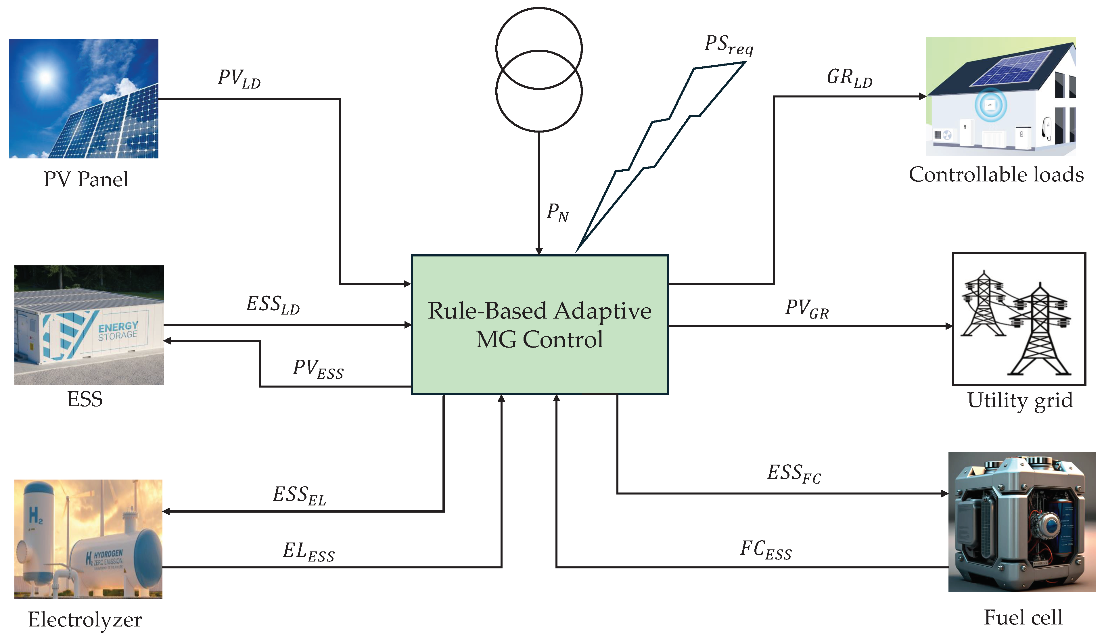
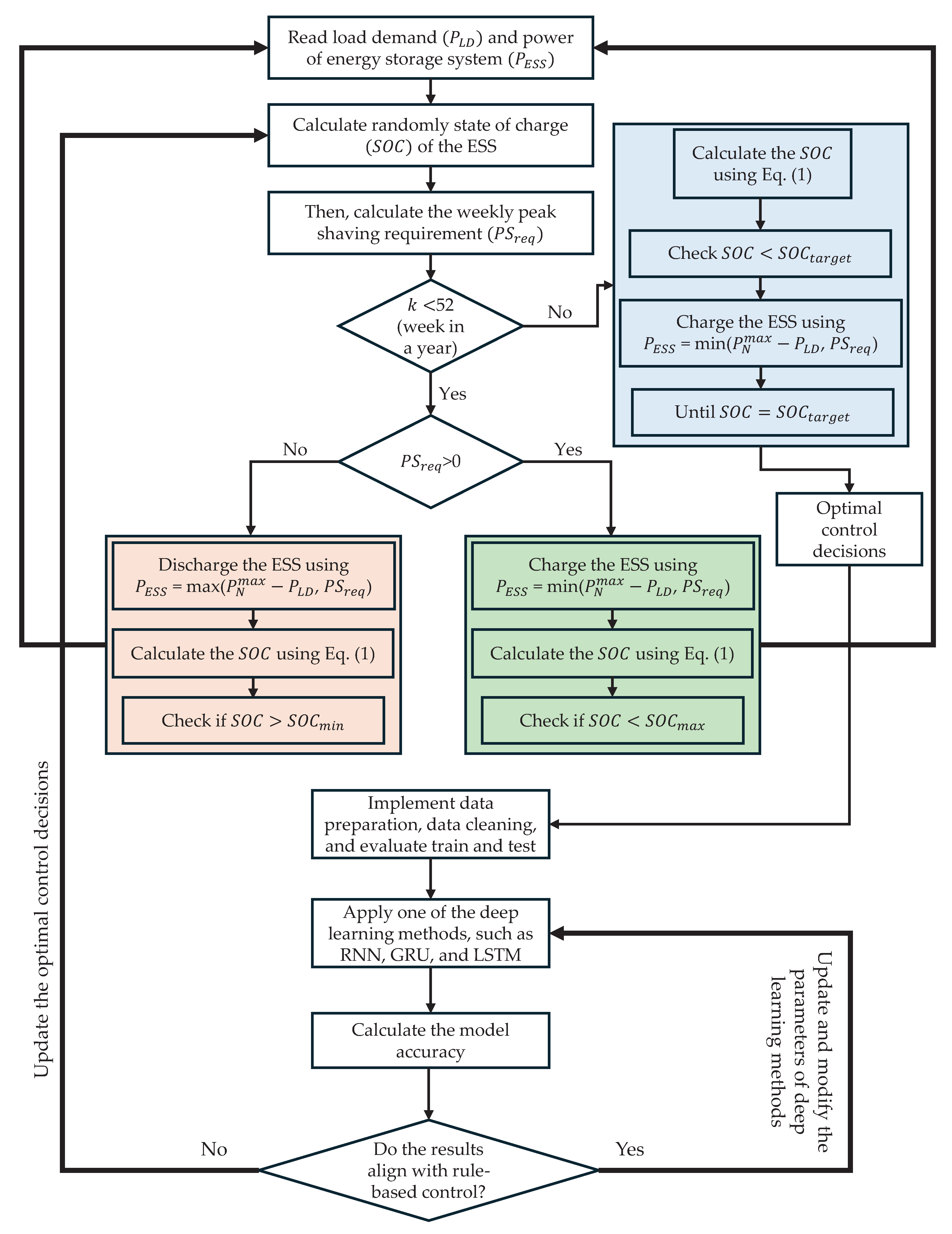
2.1. Rule-Based Control

Figure 1 represents the adaptive MG structure controlled in this paper. The MG is composed of PV, grid (GR), ESS, load (LD), electrolyzer (EL), and fuel cell (FC). The ESS is composed of a battery (BAT), fuel tank (FT), and water tank (WT). The MG’s ESS reduces peak demand from a cluster of loads in the distribution network [46].

P_{L D}

stands for the total demand of these loads, while

P_{N}

represents the power obtained from the upstream network, constrained by the network operator’s set boundaries (

P_{N}^{m a x}

). The symbols

η_{c h}

and

η_{d i s}

denote the efficiency of the ESS during the charging and discharging phases, respectively. C represents the nominal capacity of the ESS, expressed in kWh.

P_{E S S} (k)

denotes the power exchanged with the network during the current operational time. A positive value of

P_{E S S} (k)

indicates the charging state, while a negative value indicates the discharging state. The State of Charge (

S O C

) during the current operational period (k) is determined by the energy exchanged through the ESS and its value from the previous period (k-1).

The rule-based EMS controls the ESS, which uses the measured values of

P_{L D}

and

P_{E S S}

to establish the proper set-point for power exchange. Figure 2’s flow chart shows this EMS, emphasising the importance of

S O C

as a critical parameter for sending control commands. Utilising the following relationships, the

S O C

of the ESS during the current operational period (k) is determined by the energy exchanged through the ESS. It is calculated using the following equations:

S O C (k) = \{\begin{matrix} S O C (k - 1) + (\frac{P_{E S S} (k) \cdot η_{c h} \cdot k}{C}) & if P_{E S S} (k) > 0 \\ S O C (k - 1) + (\frac{P_{E S S} (k) \cdot k}{C \cdot η_{d i s}}) & if P_{E S S} (k) < 0 \end{matrix}

(1)

The illustrated EMS has an hourly control horizon and weekly operational periods (k), which need the EMS to take the necessary control actions. By maintaining a 50%

S O C

at the end of the control horizon, the ESS will have enough energy reserves to provide peak reduction in the following days. It is considered that the distribution network’s chosen location for peak reduction services, with a

S O C

ranging from 20% to 100%, has an ESS that is optimally sized to support it. The purpose of setting the bottom boundary of the

S O C

is to guarantee the ESS runs smoothly. In order to ensure effective operation and peak demand mitigation, the rule-based EMS uses measured values of

P_{E S S}

and

P_{L D}

to calculate the optimal power exchange set-point for the ESS.

Furthermore, since the main goal is to determine the best imputation technique for missing data within the ESS, it is assumed that there are no missing values in

P_{L D}

The control decisions of the adaptive MG are defined to find the optimum system control, state, and output vectors for the rule-based control.

Define the adaptive MG’s system-state, control, and output vectors with the help of Equation (1):

x (k) = [S O C^{E S S} (k)]

(2)

where

S O A c c^{E S S} (k)

is the state of charge for the ESS.

The system-control (input) vector of the adaptive MG is defined as follows:

u (k) = [P V_{L D} (k); P V_{G R} (k); P V_{E S S} (k); E S S_{L D} (k)]

(3)

where

P V_{L D}

P V_{G R}

, and

P V_{E S S}

are the power flow from PV to the LD, GR, and ESS, respectively.

E S S_{L D}

is the power flow from the ESS to the LD. In this case, the ESS is in discharge mode.

The system-output vector of the adaptive MG is as follows:

y (k) = [G R_{L D} (k); E S S_{G R} (k)]

(4)

where

G R_{L D}

is the power import from the GR for the LD and

E S S_{G R}

is the power flow from the ESS to the GR.

Define the objective functions for the rule-based control on the adaptive MG:

The power imported from the utility grid is minimized.

$m i n J_{1} (k) = m i n \sum_{k}^{k + N_{c}} {(P_{L D} (k) - (P V_{G R} (k) + E S S_{G R} (k) + G R_{L D} (k)))}^{2}$

(5)
The usage of the ESS is penalized to prevent the charging from the utility grid.

$m i n J_{2} (k) = m i n \sum_{k}^{k + N_{c}} {(P V_{E S S} (k) - (E S S_{L D} (k) + E S S_{G R} (k)))}^{2}$

(6)
The exported energy to the utility grid is encouraged.

$m i n J_{3} (k) = m i n \sum_{k}^{k + N_{c}} {(P_{P V} (k) - (P V_{E S S} (k) + P V_{G R} (k)))}^{2}$

(7)

By merging Equations (5)–(7), the overall cost function (objective function) for the adaptive MG:

m i n J (k) = m i n (J_{1} (k) + J_{2} (k) + J_{3} (k))

(8)

Define the constraints for the adaptive MG as follows:

Power flows from the PV, GR, and ESS are non-negative values and are subject to their maximum values.

\begin{matrix} 0 \leq P V_{L D} (k) \leq P V_{L D}^{max} \\ 0 \leq P V_{G R} (k) \leq P V_{G R}^{max} \\ 0 \leq P V_{E S S} (k) \leq P V_{E S S}^{max} \\ 0 \leq G R_{L D} (k) \leq G R_{L D}^{max} \\ 0 \leq E S S_{G R} (k) \leq E S S_{G R}^{max} \\ 0 \leq E S S_{L D} (k) \leq E S S_{L D}^{max} \end{matrix}

(9)

The sum of the PV energy supplied directly for the LD

(P V_{L D})

, the ESS for the charging

(P V_{E S S})

, and the energy exported to the GR

(P V_{G R})

should be smaller than the energy flow from the PV array,

(P_{P V} (k))

P V_{L D} (k) + P V_{E S S} (k) + P V_{G R} (k) \leq P_{P V} (k)

(10)

Also, the sum of the LD from the PV and ESS should equal the building’s load demand.

P V_{L D} (k) + E S S_{L D} (k) + G R_{L D} (k) \leq P_{L D} (k)

(11)

The

S O A c c^{E S S}

for the ESS is restricted between its minimum and maximum values.

S O A c c^{{E S S}^{m i n}} \leq S O A c c^{E S S} \leq S O A c c^{{E S S}^{m a x}}

(12)

Charging and discharging for the ESS cannot happen simultaneously, as is implied by the following:

\begin{matrix} P V_{E S S} (k) E S S_{L D} (k) \leq 0 \\ P V_{E S S} (k) E S S_{G R} (k) \leq 0 \end{matrix}

(13)

It is worth noting that Equations (9)–(12) are convex, whereas Equation (13) is non-convex. In order to accomplish convex optimization in rule-based control design, the non-convex constraints into two switched cases: (i) charging: (

E S S_{L D} = 0

and

E S S_{G R} = 0

) and (ii) discharging: (

P V_{E S S} = 0

Charging: The constraint can be re-written by:

$\begin{matrix} \begin{matrix} E S S_{L D} (k) \leq 0 E S S_{L D} (k) \geq 0 \\ E S S_{G R} (k) \leq 0 E S S_{G R} (k) \geq 0 \end{matrix} \end{matrix}$

(14)

Constraints (9)–(11), and (14) can be compactly re-written by:

$\begin{matrix} μ_{c h} u (k) \leq γ_{c h} \end{matrix}$

(15)

where

$μ_{c h} = [\begin{matrix} - e y e (6) \\ 0 & 0 & 0 & 1 & 0 & 0 \\ 1 & 1 & 0 & 0 & 0 & 1 \\ 1 & 0 & 1 & 1 & 0 & 0 \\ e y e (6) \\ - 1 & - 1 & 0 & 0 & 0 & - 1 \end{matrix}] γ_{c h} = [\begin{matrix} z e r o s (6, 1) \\ 0 \\ P_{L D} (k) \\ P_{P V} (k) \\ P_{m}^{m a x} o n e s (6, 1) \\ P V_{G R}^{m a x} - P_{L D} (k) \end{matrix}]$

where $e y e$ is an identity matrix, and $z e r o s$ is creating an array of all zeros.
Discharging: The constraint can be re-written by:

$\begin{matrix} \begin{matrix} P V_{E S S} (k) \leq 0 P V_{E S S} (k) \geq 0 \end{matrix} \end{matrix}$

(16)

Constraints (9)–(11) and (16) can be compactly re-written by:

$μ_{d i s} u (k) \leq γ_{d i s}$

(17)

where

$μ_{d i s} = [\begin{matrix} - e y e (6) \\ 0 & 0 & 0 & 0 & 1 & 1 \\ 1 & 1 & 0 & 0 & 0 & 1 \\ 1 & 0 & 1 & 1 & 0 & 0 \\ e y e (6) \\ - 1 & - 1 & 0 & 0 & 0 & - 1 \end{matrix}] γ_{c h} = [\begin{matrix} z e r o s (6, 1) \\ 0 \\ P_{L D} (k) \\ P_{P V} (k) \\ P_{m}^{m a x} o n e s (6, 1) \\ P V_{G R}^{m a x} - P_{L D} (k) \end{matrix}]$

2.2. General Formulations of Deep Learning Techniques

Deep learning models are crucial for improving the control system’s intelligence and adaptability. These models capture intricate patterns and correlations by using the benefits of the temporal dependencies included in the data, allowing for real-time, updated control decisions. The hybrid control system includes integrations with the subsequent deep learning architectures:

2.2.1. Long Short Term Memory

LSTM networks are a form of RNN architecture that addresses the vanishing gradient problem and captures long-range dependencies in sequential input. LSTMs have specialised memory cells and gating mechanisms that allow them to retain and update information selectively across several steps.

The LSTM computation for each time step (k) is defined as:

h (k + 1) = LSTM (u (k + 1), h (k), c (k)) .

where

u (k)

is the input,

h (k)

is the hidden state, and

c (k)

is the cell state. The cell state serves as a long-term memory component, storing information across time, whilst the hidden state catches and transports short-term dependencies.

The LSTM architecture has three main gates: the input gate (

u (k)

), the forget gate (

f (k)

), and the output gate (

y (k)

. These gates control the flow of information into, out of, and within the LSTM cell, allowing it to filter out irrelevant facts while retaining useful information. Furthermore, LSTM cells have an internal memory cell (

u (k)

) that allows them to store and update data with time.

LSTM networks excel at capturing long-range dependencies, making them appropriate for tasks involving sequential data and complex temporal dynamics. In a hybrid control system, LSTM models are critical for learning and anticipating the temporal behaviour of the MG system. LSTM-based control strategies improve the adaptability and performance of the hybrid control system by efficiently capturing and utilising temporal relationships, resulting in increased efficiency and stability during MG operation.

2.2.2. Gated Recurrent Unit

GRU networks are a type of RNN architecture that looks like LSTM but has a simpler topology. GRUs are intended to capture long-term dependencies in sequential data while remaining computationally more efficient than LSTMs.

At each time step (k), the GRU computation is described as follows:

h (k + 1) = GRU (u (k + 1), h (k))

Unlike LSTM cells, GRU cells lack discrete memory cells and instead use a single concealed state to record both short-term and long-term reliance.

The GRU architecture consists of two primary gates: the reset gate (

r (k)

) and the update gate (

z (k)

. These gates, which regulate information flow within the GRU cell, allow the hidden state to be selectively updated based on the input and previous hidden states. The update gate determines how much of the new data should be absorbed, whereas the reset gate specifies how much of the old disguised state should be forgotten.

GRU networks achieve a balance between model complexity and performance, thereby being appropriate for tasks involving sequential data of intermediate complexity. In the context of a hybrid control system, GRU-based models provide an efficient and effective way to capture temporal dependencies and make sound control decisions. By exploiting GRU network capabilities, the hybrid control system improves adaptability and performance, increasing efficiency and stability in MG operation.

2.3. Integration of Rule-Based Control with Deep Learning Techniques

All experiments are run on an NVIDIA A100 and two Intel Xeon(R) CPUs @ 2.30GHz and 12 GB of memory. Although the data has been collected with care, some manipulations are needed. We first discuss the process used for dataset cleansing to provide data that can be fed directly to deep networks. We then cover the search space of deep learning networks, which we evaluated as part of this work.

2.4. Dataset Preprocessing

Within this phase, we consider how to prepare the data for RNN-based deep networks since the data contains the hourly power recirculation of adaptive MG systems in a year. The dataset includes 13 attributes. To better represent the data in the RNN-based models we have designed, we grouped them, as illustrated in Table 1.

Accumulated: The column $P_{L D}$ is the total need of the smart building; hence, the sum of the columns $P V_{L D}$ , $G R_{L D}$ , and $B A T_{L D}$ fulfils it. The photovoltaic energy source $P_{P V}$ distributes the power to the columns $P V_{G R}$ , $P V_{L D}$ , and $P V_{B A T}$ .
Additional elements: The power needs in these columns are at negligible levels since $W T$ , $F C$ , $E L$ , and $F T$ require a small amount of power for ignition.
Main elements: Since the presented smart building system mainly circulates power within LD, PV, GR, and BAT, the corresponding columns are considered the main elements.

As a result of the aforementioned details and correlation analysis (Figure 3),

P V_{G R}

P V_{L D}

G R_{L D}

P V_{B A T}

, and

B A T_{L D}

are left to be used in RNN models. Moreover, the first RNN-based models were trained using the different data portions to see the real-time effects of eliminated columns. Because these experiments resulted in negative

R^{2}

values, it is considered that the column elimination process is cross-checked.

Several notable correlations are observed within the dataset in Figure 3. For instance, there is a strong positive correlation between power supplied by photovoltaic (PV) systems and the actual PV power generated (

P_{P V}

), as expected. Additionally, the power consumed from the grid (

G R_{L D}

) exhibits a significant positive correlation with power consumption (

P_{L D}

), indicating that grid power is a substantial contributor to the overall power consumption in the building.

Interestingly, there are negative correlations between certain attributes, such as between battery power consumption (

B A T_{L D}

) and power consumption from fuel cells (

F C_{B A T}

). This suggests that when one power source is utilized more, the other may be utilized less, indicating a potential trade-off or balancing act in power usage within the building.

Figure 4 depicts a comprehensive picture of power dynamics within the smart building, highlighting various properties across different time intervals. Several major observations arise from extensive research and are backed by particular numerical results:

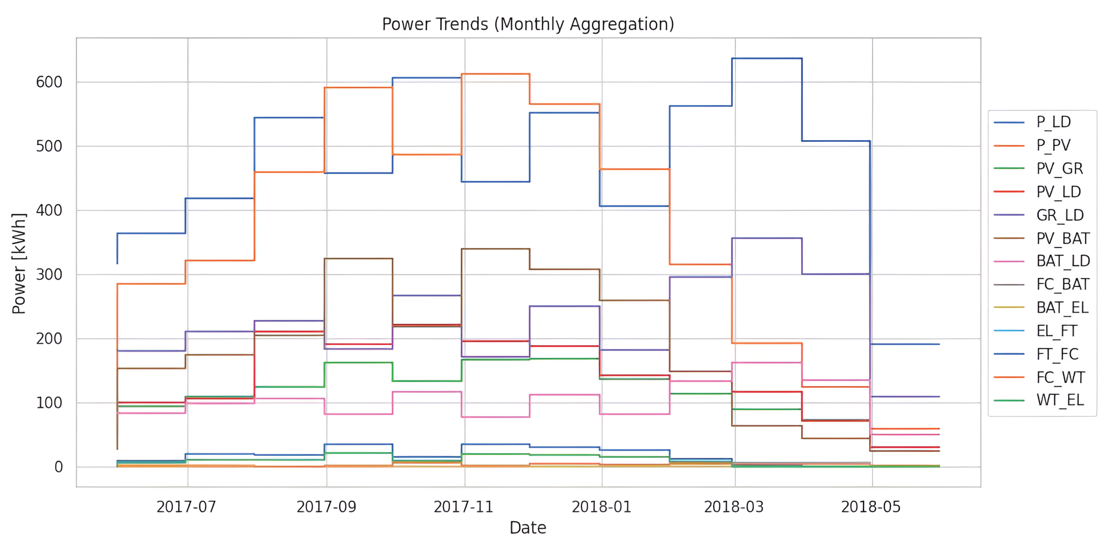
Significant changes in power qualities are found during different time periods. For example, on May 31, 2017, total power usage was 316.75 kWh, with PV generation accounting for 83.65 kWh, power from PV to the grid ( $P V_{G} R$ ) (44.65), and electricity from PV to local distribution ( $P V_{L} D$ ) (49.90 kWh). In contrast, on March 31, 2018, overall power consumption increased to 635.77 kWh, accompanied by changes in PV generation (192.31 kWh) and other power distribution components.
Seasonal variations are evident in the dataset, with distinct trends observed across different months. For example, during the summer months, such as June and July 2017, both power consumption and generation peaked, indicating higher energy demand and increased solar irradiance. Conversely, in winter months, such as December 2017, power consumption remained relatively stable, while PV generation decreased due to reduced daylight hours.
Figure 4 underscores the role of RESs in power generation. For instance, on April 30, 2018, the PV contributed significantly to overall power generation, with PV generation reaching 124.53 kWh and WT to EL ( $W T_{E L}$ ) at 0.33 kWh. These assets are crucial in reducing dependency on conventional grid power and mitigating environmental impact.
ESSs, particularly batteries, facilitate efficient power management within the smart building. Notably, while certain power components such as $F C_{B A T}$ , $B A T_{E L}$ , $E L_{F T}$ , $F T_{F C}$ , $F C_{W T}$ , and $W T_{E L}$ are essential for energy transfer and system operation, their individual contributions to overall power consumption and generation are minimal. For instance, on May 31, 2017, $F C_{B A T}$ , $B A T_{E L}$ , $E L_{F T}$ , $F T_{F C}$ , $F C_{W T}$ , and $W T_{E L}$ collectively accounted for less than 1 kWh of power transfer.

In conclusion, the numerical results from the dataset provide valuable insights into the dynamics of power circulation within the smart building, emphasizing the importance of renewable energy integration, energy storage technologies, and efficient energy management practices. Further analysis and modelling based on this data can inform the development of sustainable and resilient smart building systems tailored to specific energy needs and environmental considerations.

2.5. Model and Hyperparameter Search

Deep learning networks’ shape (layers and neurons per layer) significantly impacts performance [47]. We perform a search space for the most suitable solution for the obtained data. In order to prevent confusion from now on, we use the term RNN-based for all recurrent types of architectures. Since the possibility pool for experimental sets to be created with combinations of different parameters is infinite, we focused mainly on the effects of the types and number of RNN units, including the number of hidden states, optimizers, and learning rate schedulers.

2.5.1. RNN-Based Architectures:

We identify three different variants of RNN-based approaches: Simple RNN (sRNN), LSTM and GRU. The number of hidden states is restricted between 1 and 3. Initially, we started the experiments using the number of units in the hidden layers selected as multiples of the number of columns of the input data.

2.5.2. Optimizers:

The optimizer decides how the neural network weights are adjusted following each training iteration. This study concentrates on three widely employed optimizers:

SGD (Stochastic Gradient Descent): SGD is the primary optimizer employed in Deep Learning. Although Gradient Descent theoretically updates the weights after processing each training sample, it is common to optimise the weights after processing each batch of data.

RMSprop (Root Mean Squared Propagation): RMSprop improves the performance of stochastic gradient descent (SGD) by including fading average partial gradients to adapt the step size of each parameter. This optimizer prioritises recent gradients to a greater extent.

Adam (ADAptive Moment estimation) [48]: Adam, like RMSprop, allocates specific learning rates to each parameter. While RMSprop calculates the average of the first moment, Adam takes into account the average of the second moment as well when adjusting the learning rates.

2.5.3. Learning Rate Schedulers:

Learning rate schedules aim to modify the learning rate when training by reducing the rate per a predetermined schedule. In this study, we used 4 common approaches:

Constant: As the name implies, in this scheduler, the model does not change the rate of the learning rate during the training phase. We accept the default value as 0.001.

Time-Based Decay: This approach intends to reduce the learning over epochs as seen in Equation 18. While

l r

and k are hyperparameters, the current learning and decay rates, t is the iteration number. As in the constant learning rate scheduler, we assign 0.001 as the initial learning rate. The decay rate is found by dividing the current learning rate by the current number of the epoch.

l r = \frac{l r_{0}}{(1 + k t)}

(18)

Step Decay: This learning rate schedule, where the number of epochs is a hyperparameter, reduces the learning rate by a factor every few epochs.

Exponential Decay: This schedule applies an exponential decay function to an optimizer step, based on a defined initial learning rate, as described in Equation 19.

l r = \frac{l r_{0}}{e^{(- k t)}}

(19)

2.6. Implementation Details

We use an 80-20 training test split. Further, the training data is split into training and validation sets of 80% and 20%, respectively. When we refer to ’batch size’ in the context of data analysis, it indicates the number of consecutive data points grouped together for processing. For instance, if we select a batch size of 7 for daily power consumption data, we organise the yearly dataset into segments of 7 consecutive days each. Each segment represents a week’s worth of data. This approach facilitates the computational learning process by enabling the models to discern patterns and trends occurring every week. Therefore, opting for a batch size of 7 assists in examining and understanding the weekly variations in power consumption.

We employ the Glorot uniform initializer [49] to initialize the parameters within our networks. This initializer ensures that the weights are uniform across all layers regarding the variance of the activations, thereby preventing the gradient from either exploding or vanishing due to a consistent variance. After eliminating unnecessary columns, we obtained 5 columns, as mentioned earlier, and hence, the output dense layer has 6 neurons.

After the first attempts, we discovered that the high number of epochs did not perform satisfactorily; thus, we kept it constant at 20. In addition, the constant learning rate performed better among other candidates, such as Time-Based Decay, Step Decay, and Exponential Decay.

Finally, the activation function provides the non-linear element within the networks. Due to the nature of the case, the power consumption predictions in the output-dense layer should not produce negative values. To overcome this issue, we used ReLU. On the other hand, the activation functions of RNN-based layers were not interfered with.

Finally, the hidden state is defined to update the control decision of the proposed method. It is

h (k)

at time step k and depicts the adaptive MG system’s dynamics as learned by the RNN model. It encodes information about the MG system’s current state using past observations and inputs.

The hidden state,

h (k)

, can be defined as follows:

h (k) = [S O C^{E S S} (k)]

(20)

The hidden state captures the current SOC of the ESS, providing information about the energy storage level and potentially other relevant variables affecting the MG system dynamics.

In LSTM networks, the cell state

c (k)

at time step k functions as a long-term memory component and complements the hidden state. It allows the model to capture long-range dependencies in the sequential data by storing and updating data over numerous time steps.

The cell state

c (k)

in this situation can be described as follows:

c (k) = [f_{G R_{L D} (k)}, f_{E S S_{G R} (k)}]

(21)

The forward-passed features

f_{G R_{L D}}

and

f_{E S S_{G R}}

represent the power flows from the GR to the LD and ESS to the GR. These features collect essential information about the MG system’s power consumption and storage dynamics, which helps the model predict future states and make control decisions.

In summary, the rule-based control logic serves as a basic control method, providing a framework for decision-making in the MG system. It can handle known scenarios and take prompt action based on specified rules. Deep learning models are used to supplement rule-based control by learning from data and delivering adaptive control actions in instances when rules may be insufficient or when the system confronts unexpected conditions. Deep learning models can detect complicated patterns and non-linear correlations in data and optimise control decisions. Then, a decision-making mechanism is created that dynamically switches between rule-based control and deep learning models based on the MG system’s current state, performance metrics, or other relevant variables. For instance, the system may use rule-based control under typical settings but switch to deep learning models when there is a lot of ambiguity or when dealing with new scenarios. Next, the integrated control strategy will be tested through simulation or real-world testing to confirm that it meets the MG system’s objectives and criteria. Following that, its performance will be evaluated in terms of stability, efficiency, dependability, and flexibility in various working environments. To improve the iterative process, regularly monitor and analyse the performance of the integrated control strategy while gathering feedback from the adaptive MG system. Use this feedback to improve overall system performance by refining rule-based control logic, fine-tuning deep learning models, or adjusting the decision-making mechanism. By integrating rule-based control and deep learning methods, we can use both approaches to provide a more resilient, adaptive, and economical control strategy for the adaptive MG system.

3. Results and Discussions

3.1. The Results of the Rule-Based Control

This section examines the performance of the rule-based control system in managing energy consumption and storage within the smart building. The basic rule-based control system relies on predetermined rules and thresholds, with no machine learning or predictive modelling capabilities. We assess its performance by analysing weekly load demand data, ESS configurations, and SOC metrics.

The weekly load demand represents the total power consumption within the smart building for that week, whereas the ESS configurations represent changes in energy storage capacity caused by charging or discharging activities. The SOC represents the proportion of energy stored compared to the ESS’s full capacity.

Figure 5a illustrates how analysing weekly load demand and ESS configurations reveals patterns in energy use and storage behaviour. During weeks with higher load needs, the ESS configurations are adjusted to meet the increasing energy requirements. Conversely, periods with reduced load demands may see ESS charging activities to optimise energy utilisation and sustain SOC levels. Figure 5b shows that in weeks with high load demand, such as the 1st, 11th, and 42nd weeks, ESS configurations discharge more to meet energy demands. In contrast, during weeks with reduced load needs, such as the 35th and 48th weeks, the ESS setups demonstrate decreased discharge or even charging activities to maintain SOC values.

Figure 5c illustrates how the basic rule-based control system effectively manages energy storage and optimises SOC levels. By keeping SOC within optimal ranges, the system maintains sufficient energy reserves to satisfy future load demands while preventing overcharging or discharging of the ESS. Analysis of SOC measurements shows that the rule-based control system effectively keeps SOC within acceptable limits, assuring the ESS’s operational efficiency and durability. Throughout the monitoring period, SOC levels remained within the prescribed range, showing that energy storage resources were successfully managed.

The findings illustrate the effectiveness of the rule-based control system in regulating energy storage and consumption in the context of smart buildings. The system adapts to ranging load requirements by utilising predetermined regulations and thresholds and optimises energy consumption while preserving SOC levels within preferred intervals. However, it is essential to acknowledge the limitations of rule-based control systems, particularly in handling complex and dynamic environments. While effective for basic energy management tasks, rule-based systems may struggle to adapt to unforeseen circumstances or optimize energy usage based on historical data alone.

Next, the integration of machine learning techniques, such as predictive modelling and reinforcement learning, has been implemented to enhance the adaptability and intelligence of EMSs. By combining the strengths of rule-based control with the learning capabilities of machine learning algorithms, a hybrid approach known as hybrid intelligent control could offer superior performance and flexibility in managing smart building energy systems.

3.2. The Results of the Deep Learning Methods

We present the results of our model training. The main evaluation metrics are selected as

R^{2}

, Mean Squared Error (MSE), and Mean Absolute Error (MAE). The evaluation metrics were obtained from test scores. Table 2 presents the top 20 performing models.

Here we present the architectural notation. Our neural network architecture consists of multiple recurrent layers, each with a customizable number of hidden states. Each integer value in brackets after the corresponding recurrent layers presents the number of units of the hidden state. Corresponding to this, e.g., LSTM(50) + LSTM(50), means the model has two hidden states with 50 units each.

Considering the top 20 cases in Table 2, none of the recurrent layers overwhelms the others. The best case was obtained from the single GRU with 50 units with ∼0.99

R^{2}

, almost 0 MSE, and MAE.

We now summarise other design choices:

Optimizer: The experiments showed that none optimizers can be considered better than the others. Although the number of occurrences of SGD seems lower than the others, it is still a suitable candidate.
Learning Rate Scheduler: The constant learning rate schedule dominates the results.
Deepness of the Architecture: Considering the data set used, it has been observed that relatively shallow models give better results, regardless of the recurrent layer type.

3.2.1. Threats to Validity

In this section, we outline the constraints of the experimental part of our study and emphasize potential validity concerns stemming from these limitations. Our methodology is shaped by comparable endeavours in the systems performance literature (such as Eismann et al.[50]) and follows the approach adopted by Wohlin et al.[51].

L1 Infinite search space: Several factors limit the RNN-based model training process.
L2 Obtained results: This study is not a benchmarking of various models.
L3 Single power consumption dataset: This study uses only data from a single smart building.
L4 Single expert for model training: Although the search space has been discussed collaboratively, a single expert conducted the experimental designs of RNN-based models.

Now, let us examine the consequences of these constraints in relation to the concepts of search space, outputs, internal, and external validity.

Search Space: Even though there is a possibility of obtaining more promising models with other parameter combinations (Limitation L1), this study mainly focused on improving promising model designs.

Outputs: In the process of finding the most suitable RNN-based model for the data, the models that gave the best results (Limitation L2) in terms of evaluation metrics were taken into account.

Internal Validity: Our work involved cleaning the data to be amenable to analysis and machine learning. A single expert researcher observed the effects of eliminated columns in RNN-based models (Limitation L4), leaving the opportunity to misinterpret the columns. The processes undertaken were well documented to mitigate this impact, and two further researchers audited the process. The code of the whole process is made available to the community1.

External Validity: This work concerns the prediction of power consumption results from a single dataset, (Limitation L3). Further work could have also evaluated whether to extend the existing data or add more data from various smart buildings.

3.3. The Results of the Hybrid Intelligent Control

The weekly data for power attributes, including

P_{P V}

G R_{L D}

P V_{L D}

, and

B A T_{L D}

, provide valuable insights into the energy dynamics of the smart building. Our proposed method significantly improves energy management and efficiency by leveraging a combination of rule-based control and deep learning techniques.

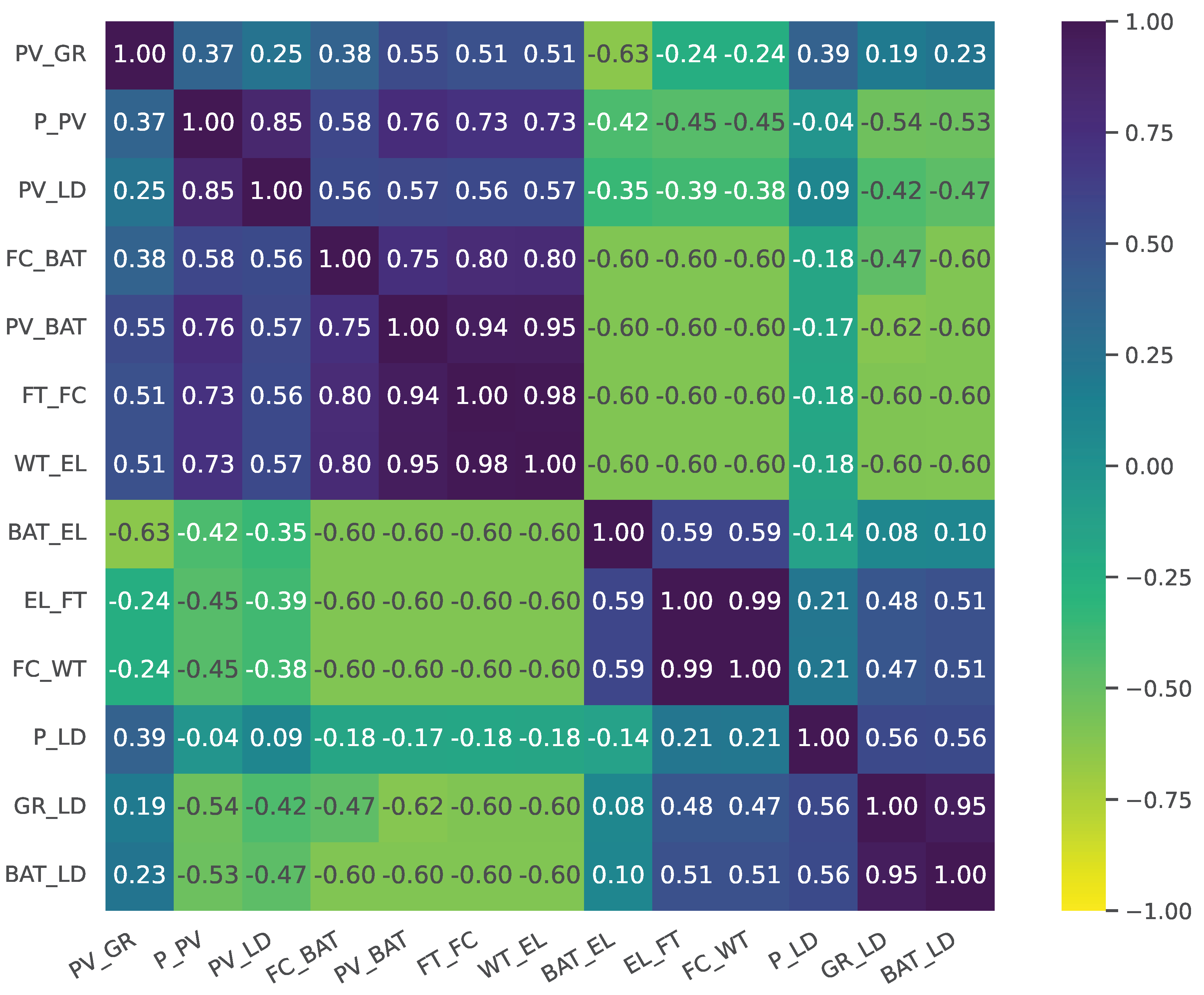
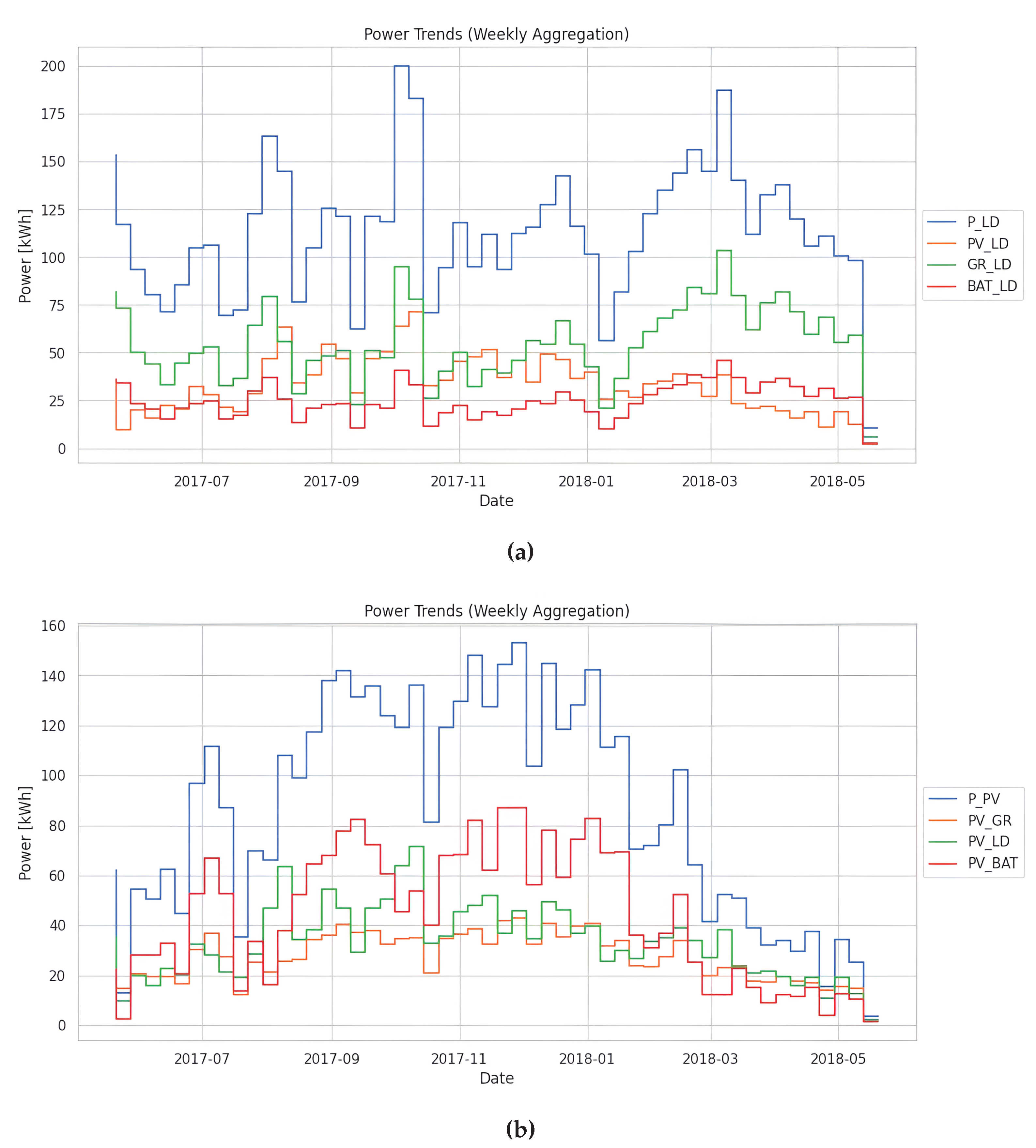
The weekly variations in power attributes reveal distinct patterns over time. By integrating rule-based control strategies, such as scheduling power generation and consumption based on predicted demand, the system optimizes energy utilization while minimizing wastage. For example, on June 4, 2017, $P V_{L D}$ and $G R_{L D}$ exhibited lower values than in previous weeks, indicating potential energy savings through load shifting or demand response mechanisms (see Figure 6a).
Deep learning techniques enhance the system’s predictive capabilities, enabling accurate forecasting of power generation and consumption patterns. Through RNNs or LSTM models, the system can adapt to dynamic changes in energy demand and supply, optimizing decision-making processes in real-time. For instance, as shown in Figure 6b, on August 13, 2017, the system accurately predicted an increase in power consumption, allowing proactive adjustments to grid interactions and energy storage.Deep learning models use features like $P V_{B A T}$ and $P_{P V}$ to estimate power generation and consumption trends, resulting in more accurate decision-making. On June 4, 2017, the incorporation of $P_{P V}$ data allowed the system to predict increasing PV generation and proactively modify energy distribution and storage.
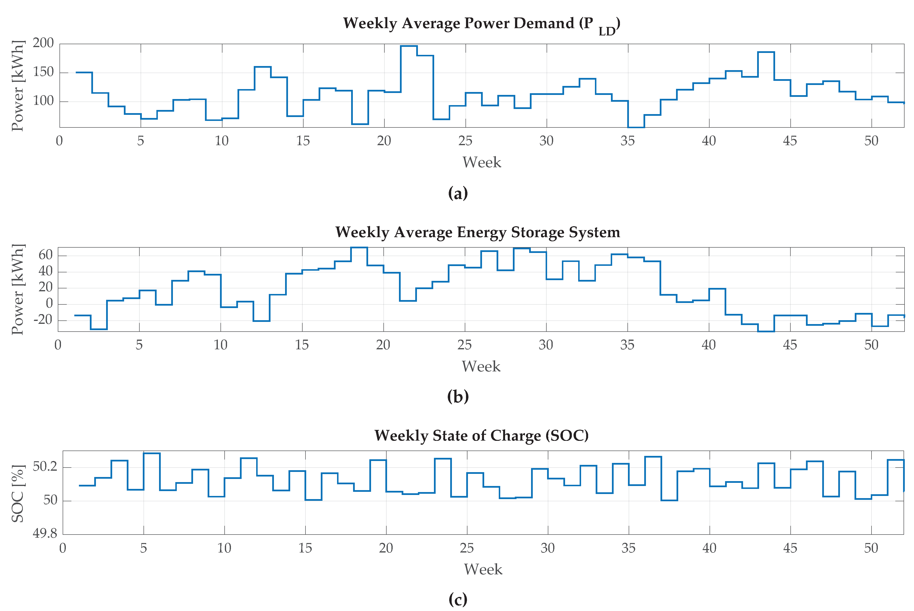
Integrating battery systems, directed by rule-based control and informed by deep learning predictions, is critical for optimising energy storage and distribution. Figure 6 shows that the system can intelligently manage battery charging and discharging cycles by considering $P V_{B A T}$ and $B A T_{L D}$ data in conjunction with other variables, such as $P V_{L D}$ and $G R_{L D}$ . The system decreases grid dependency and peak load demand by strategically charging and discharging batteries in response to predicted demand and generation. On July 30, 2017, $B A T_{L D}$ data showed effective use of battery capacity to balance changes in $P V_{L D}$ and $G R_{L D}$ .
The combination of basic rule-based control and deep learning provides synergistic benefits for energy management. Rule-based algorithms give deterministic guidance for system operation, but deep learning models improve adaptability and responsiveness to changing environmental conditions. By combining the benefits of both techniques, the system reaches peak energy efficiency, cost savings, and environmental sustainability performance.
Our proposed solution is scalable and adaptable to various energy conditions and building environments. The system is adaptable to changing energy demands, renewable energy sources, and grid interactions, whether deployed in a residential, commercial, or industrial scenario. Furthermore, constant learning and refining of deep learning models ensures robustness and resistance to changing energy issues.

To summarise, combining the basic rule-based control and deep learning techniques into EMSs is a potential strategy for optimising power utilisation in smart buildings. The weekly power data analysis demonstrates the efficacy of our proposed strategy for increasing energy efficiency, lowering operational costs, and achieving sustainability goals. Further research and implementation initiatives can use these insights to encourage innovation in adaptive MG systems, resulting in a greener and more resilient energy future.

4. Conclusions

In conclusion, we found crucial variables in the dataset that have a substantial impact on power dynamics in adaptive MG systems through correlation analysis and numerical validation. RNN models include attributes such as

P V_{G R}

P V_{L D}

G R_{L D}

P V_{B A T}

, and

B A T_{L D}

because to their correlation and predictive power. The correlation matrix (Figure 3) indicates significant connections between several power circulation variables, offering vital insights for designing predictive models and optimising power management strategies in smart buildings. One notable association is the positive relationship between grid power consumption (

G R_{L D}

) and overall power consumption (

P_{L D}

). Negative correlations between variables, such as battery power consumption (

B A T_{L} D

) and power consumption from fuel cells (

F C_{B} A T

), indicate potential trade-offs or balancing acts in power usage inside the building.

In the context of model development, our experiments with RNN-based architectures and hyper-parameter optimization have yielded promising results. The top-performing models, as summarized in Table 2, exhibit high

R^{2}

values and low MSE and MAE, indicating their efficacy in predicting power consumption and generation within the adaptive MG systems.

Key insights from our analysis include:

The choice of optimizer and learning rate scheduler has a significant impact on model performance, with the constant learning rate scheduler consistently outperforming other schedules.
Shallow RNN architectures with relatively few hidden states yield better results than deeper architectures.
No single recurrent layer type (e.g., Simple RNN, LSTM, GRU) emerges as superior, suggesting that the choice of architecture should be tailored to the specific characteristics of the dataset and modelling task.

Our proposed method, hybrid intelligent control for adaptive MG optimization, integrates rule-based control strategies with deep learning techniques to optimize power management within adaptive MG systems. This innovative approach leverages the strengths of both rule-based systems and machine-learning algorithms to achieve adaptive and efficient energy management.

In future developments, enhancing visualization techniques [52] could significantly augment the effectiveness of energy management systems within smart buildings. Integrating predictive analytics and machine learning algorithms into visualization platforms can enable forecasting of future energy demand and generation patterns. By leveraging historical data and predictive models, stakeholders can anticipate fluctuations in energy usage, optimize resource allocation, and proactively address energy management challenges.

Author Contributions

Conceptualization, O.A., M.C. and M.C.; methodology, O.A., M.C.; software, M.C. and M.C.; validation, O.A., M.C. and M.C.; formal analysis, M.C.; investigation, M.C. and M.C.; data curation, M.C. and M.C.; writing—original draft preparation, O.A., M.C. and M.C.; writing—review and editing, O.A., M.C., M.C, A.A., D.G., and M.F.; visualization, O.A., M.C. and M.C.; supervision, A.A., D.G., and M.F.; funding acquisition, O.A.

Funding

This research was funded by Newcastle University, UK.

Institutional Review Board Statement

Not applicable.

Informed Consent Statement

Not applicable.

Data Availability Statement

Not applicable.

Acknowledgments

We thank the Ministry of National Education, Turkey for financially supporting Osman Akbulut, Muhammed Cavus, and Mehmet Cengiz’s PhD study at Newcastle University, UK.

Conflicts of Interest

The authors declare no conflicts of interest.

Abbreviations

The following abbreviations are used in this manuscript:

BAT	Battery
CS	Cuckoo Search
EL	Electrolyzer
EMS	Energy Management System
ESS	Energy Storage System
FC	Fuel cell
FT	Fuel tank
GR	Grid
GRU	Gated Recurrent Unit
GOA	Grasshopper Optimization Algorithm
HRES	Hybrid Renewable Energy System
LD	Load
LSTM	Long Short-Term Memory
MAE	Mean Absolute Error
MG	Microgrid
MSE	Mean Squared Error
MPC	Model Predictive Control
MS	Master-Slave
PD	Primal-dual
PSO	Particle Swarm Optimization
PV	Photovoltaic
RES	Renewable Energy Sources
RNN	Recurrent Neural Network
S-MPC	Switched Model Predictive Control
sRNN	Simple Recurrent Neural Network
TLBO	Teaching Learning-based Optimization
WT	Water tank
$B A T_{L D}$	Power flow from the BAT to the LD
$B A T_{L D}^{m a x}$	The maximum power flow the BAT to the LD
$B A T_{E L}$	Power flow from the BAT to the EL
C	Battery Capacity
$c (k)$	Internal memory cell at k
$E L_{F T}$	Power flow from the EL to the FT
$f (k)$	Forget gate at k time step

$F C_{B A T}$	Power flow from the FC to the BAT
$F C_{W T}$	Power flow from the FC to the WT
$F T_{F C}$	Power flow from the FT to the FC
$G R_{L D}$	Power flow the GR to the LD
$G R_{L D}^{m a x}$	The maximum power flow the GR to the LD
$h (k)$	Hidden state at k time step
$J (k)$	Cost function
$N_{c}$	Control horizon
$P_{E S S}$	The nominal capacity of the ESS
$P_{L D}$	Load Demand
$P_{P V}$	Power generated from the PV
$P_{N}$	The power obtained from the upstream network
$P_{N^{m a x}}$	The network operator’s set boundary
$P V_{B A T}$	Power flow from the PV to the BAT
$P V_{B A T}^{m a x}$	The maximum power flow the PV to the BAT
$P V_{G R}$	Power flow from the PV to the GR
$P V_{G R}^{m a x}$	The maximum power flow the PV to the GR
$P V_{L D}$	Power flow from the PV to the LD
$P V_{L D}^{m a x}$	The maximum power flow the PV to the LD
$S O C$	State of Charge
$S O C^{B A T}$	The state of charge of the battery
$S O C^{B A T_{m i n}}$	The minimum of state of charge of the battery
$S O C^{B A T_{m a x}}$	The maximum of state of charge of the battery
$W T_{E L}$	Power flow from the WT to the EL
$x (k)$	State vector at k time step
$y (k)$	Output vector at k time step
$u (k)$	Input vector at k time step
$η_{c h}$	Charging efficiency of the battery
$η_{d i s}$	Discharging efficiency of the battery

References

Mannini, R.; Darure, T.; Eynard, J.; Grieu, S. Predictive Energy Management of a Building-Integrated Microgrid: A Case Study. Energies 2024, 17, 1355. [Google Scholar] [CrossRef]
Giaouris, D.; Papadopoulos, A.I.; Voutetakis, S.; Papadopoulou, S.; Seferlis, P. A power grand composite curves approach for analysis and adaptive operation of renewable energy smart grids. Clean Technologies and Environmental Policy 2015, 17, 1171–1193. [Google Scholar] [CrossRef]
Košťál, K.; Khilenko, V.; Hunák, M. Hierarchical Blockchain Energy Trading Platform and Microgrid Management Optimization. Energies 2024, 17, 1333. [Google Scholar] [CrossRef]
Giaouris, D.; Papadopoulos, A.I.; Seferlis, P.; Papadopoulou, S.; Voutetakis, S.; Stergiopoulos, F.; Elmasides, C. Optimum energy management in smart grids based on power pinch analysis. Chem. Eng. 2014, 39, 55–60. [Google Scholar]
Khawaja, Y.; Giaouris, D.; Patsios, H.; Dahidah, M. Optimal cost-based model for sizing grid-connected PV and battery energy system. 2017 IEEE Jordan Conference on Applied Electrical Engineering and Computing Technologies (AEECT), IEEE, 2017; 1–6. [Google Scholar] [CrossRef]
Bashishtha, T.K.; Singh, V.P.; Yadav, U.K.; Varshney, T. Reaction Curve-Assisted Rule-Based PID Control Design for Islanded Microgrid. Energies 2024, 17, 1110. [Google Scholar] [CrossRef]
Versaci, M.; La Foresta, F. Fuzzy Approach for Managing Renewable Energy Flows for DC-Microgrid with Composite PV-WT Generators and Energy Storage System. Energies 2024, 17, 402. [Google Scholar] [CrossRef]
Nikkhah, S.; Allahham, A.; Royapoor, M.; Bialek, J.W.; Giaouris, D. Optimising building-to-building and building-for-grid services under uncertainty: A robust rolling horizon approach. IEEE Transactions on Smart Grid 2021, 13, 1453–1467. [Google Scholar] [CrossRef]
Gadoue, S.M.; Giaouris, D.; Finch, J.W. Tuning of PI speed controller in DTC of induction motor based on genetic algorithms and fuzzy logic schemes. In Proceedings of the 5th International Conference on Technology and Automation; 2005; pp. 85–90. [Google Scholar]
Allahham, A.; Greenwood, D.; Patsios, C.; Taylor, P. Adaptive receding horizon control for battery energy storage management with age-and-operation-dependent efficiency and degradation. Electric Power Systems Research 2022, 209, 107936. [Google Scholar] [CrossRef]
Pervez, M.; Kamal, T.; Fernández-Ramírez, L.M. A novel switched model predictive control of wind turbines using artificial neural network-Markov chains prediction with load mitigation. Ain Shams Engineering Journal 2022, 13, 101577. [Google Scholar] [CrossRef]
Nikkhah, S.; Rabiee, A.; Soroudi, A.; Allahham, A.; Taylor, P.C.; Giaouris, D. Distributed flexibility to maintain security margin through decentralised TSO–DSO coordination. International Journal of Electrical Power & Energy Systems 2023, 146, 108735. [Google Scholar] [CrossRef]
Khawaja, Y.; Qiqieh, I.; Alzubi, J.; Alzubi, O.; Allahham, A.; Giaouris, D. Design of cost-based sizing and energy management framework for standalone microgrid using reinforcement learning. Solar Energy 2023, 251, 249–260. [Google Scholar] [CrossRef]
Zhu, J.; Chen, J.; Zhuo, Y.; Mo, X.; Guo, Y.; Liu, L.; Liu, M. Stochastic energy management of active distribution network based on improved approximate dynamic programming. IEEE Transactions on Smart Grid 2021, 13, 406–416. [Google Scholar] [CrossRef]
Aaslid, P.; Korpås, M.; Belsnes, M.M.; Fosso, O.B. Stochastic optimization of microgrid operation with renewable generation and energy storages. IEEE Transactions on Sustainable Energy 2022, 13, 1481–1491. [Google Scholar] [CrossRef]
Wang, X.; Hua, Q.; Liu, P.; Sun, L. Stochastic dynamic programming based optimal energy scheduling for a hybrid fuel cell/PV/battery system under uncertainty. Process Safety and Environmental Protection 2022, 165, 380–386. [Google Scholar] [CrossRef]
Pamulapati, T.; Cavus, M.; Odigwe, I.; Allahham, A.; Walker, S.; Giaouris, D. A review of microgrid energy management strategies from the energy trilemma perspective. Energies 2022, 16, 289. [Google Scholar] [CrossRef]
Spiliopoulos, N.; Sarantakos, I.; Nikkhah, S.; Gkizas, G.; Giaouris, D.; Taylor, P.; Rajarathnam, U.; Wade, N. Peer-to-peer energy trading for improving economic and resilient operation of microgrids. Renewable Energy 2022, 199, 517–535. [Google Scholar] [CrossRef]
Suresh, M.C.V.; Edward, J.B. A hybrid algorithm based optimal placement of DG units for loss reduction in the distribution system. Applied Soft Computing 2020, 91, 106191. [Google Scholar] [CrossRef]
Wang, Y.; Liu, S.; Sun, B.; Li, X. A distributed proximal primal–dual algorithm for energy management with transmission losses in smart grid. IEEE Transactions on Industrial Informatics 2022, 18, 7608–7618. [Google Scholar] [CrossRef]
Liu, L.-N.; Yang, G.-H. Distributed optimal energy management for integrated energy systems. IEEE Transactions on Industrial Informatics 2022, 18, 6569–6580. [Google Scholar] [CrossRef]
Cavus, M.; Allahham, A.; Adhikari, K.; Zangiabadia, M.; Giaouris, D. Control of microgrids using an enhanced Model Predictive Controller. IET 2022. [Google Scholar] [CrossRef]
Cavus, M.; Adhikari, A.A.K.; Zangiabadi, M.; Giaouris, D. Energy Management of Microgrids using a Flexible Hybrid Predictive Controller.
Cavus, M.; Allahham, A.; Adhikari, K.; Zangiabadi, M.; Giaouris, D. Energy management of grid-connected microgrids using an optimal systems approach. IEEE Access 2023, 11, 9907–9919. [Google Scholar] [CrossRef]
Cavus, M.; Allahham, A.; Adhikari, K.; Giaouris, D. A hybrid method based on logic predictive controller for flexible hybrid microgrid with plug-and-play capabilities. Applied Energy 2024, 359, 122752. [Google Scholar] [CrossRef]
Cavus, M.; Ugurluoglu, Y.F.; Ayan, H.; Allahham, A.; Adhikari, K.; Giaouris, D. Switched Auto-Regressive Neural Control (S-ANC) for Energy Management of Hybrid Microgrids. Applied Sciences 2023, 13, 11744. [Google Scholar] [CrossRef]
Rahmani, E.; Mohammadi, S.; Zadehbagheri, M.; Kiani, M. Probabilistic reliability management of energy storage systems in connected/islanding microgrids with renewable energy. Electric Power Systems Research 2023, 214, 108891. [Google Scholar] [CrossRef]
Zhang, X.; Guan, J.; Zhang, B. A master slave peer to peer integration microgrid control strategy based on communication. In 2016 IEEE PES Asia-Pacific Power and Energy Engineering Conference (APPEEC); IEEE, 2016; pp. 1106–1110. [Google Scholar] [CrossRef]
Pang, K.; Wang, C.; Hatziargyriou, N.D.; Wen, F.; Xue, Y. Formulation of radiality constraints for optimal microgrid formation. IEEE Transactions on Power Systems, 2022. [Google Scholar] [CrossRef]
Mansouri Kouhestani, F.; Byrne, J.; Johnson, D.; Spencer, L.; Brown, B.; Hazendonk, P.; Scott, J. Multi-criteria PSO-based optimal design of grid-connected hybrid renewable energy systems. International Journal of Green Energy 2020, 17, 617–631. [Google Scholar] [CrossRef]
Oviedo, R.J.M.; Fan, Z.; Gormus, S.; Kulkarni, P.; Kaleshi, D. Residential energy demand management in smart grids. In PES T&D 2012; IEEE, 2012; pp. 1–8. [Google Scholar]
Libao, F.J.D.; Dizon, R.O. Rule-based energy management strategy for hybrid electric road train. In 2018 IEEE 10th International Conference on Humanoid, Nanotechnology, Information Technology, Communication and Control, Environment and Management (HNICEM); IEEE, 2018; pp. 1–4. [Google Scholar]
Sanaye, S.; Sarrafi, A. A novel energy management method based on Deep Q Network algorithm for low operating cost of an integrated hybrid system. Energy Reports 2021, 7, 2647–2663. [Google Scholar] [CrossRef]
Abdul Basit, N.A.I.; Rosmin, N.; Mustaamal, A.H.; Hussin, S.M.; Said, D.M. A Simple Energy Management System for a Micro Grid System Using Rule-Based Algorithm. In Control, Instrumentation and Mechatronics: Theory and Practice; Springer, 2022; pp. 273–284. [Google Scholar]
Sansa, I.; Boussaada, Z.; Bellaaj, N.M. Solar Radiation Prediction Using a Novel Hybrid Model of ARMA and NARX. Energies 2021, 14, 6920. [Google Scholar] [CrossRef]
Brahma, B.; Wadhvani, R. Solar irradiance forecasting based on deep learning methodologies and multi-site data. Symmetry 2020, 12, 1830. [Google Scholar] [CrossRef]
Schmidt, R.M. Recurrent neural networks (rnns): A gentle introduction and overview. arXiv 2019, arXiv:1912.05911. [Google Scholar]
Amidi, A.; Amidi, S. Vip cheatsheet: Recurrent neural networks, 2018.
Nikkhah, S.; Allahham, A.; Royapoor, M.; Bialek, J.W.; Giaouris, D. A community-based building-to-building strategy for multi-objective energy management of residential microgrids. In 2021 12th International Renewable Engineering Conference (IREC); IEEE, 2021; pp. 1–6. [Google Scholar]
Pamulapati, T.; Allahham, A.; Walker, S.L.; Giaouris, D. Evolution Operator-based automata control approach for EMS in active buildings. IET, 2022. [Google Scholar]
Lee, D.; Arigi, A.M.; Kim, J. Algorithm for autonomous power-increase operation using deep reinforcement learning and a rule-based system. IEEE Access 2020, 8, 196727–196746. [Google Scholar] [CrossRef]
Chang, C.; Zhao, W.; Wang, C.; Song, Y. A novel energy management strategy integrating deep reinforcement learning and rule based on condition identification. IEEE Transactions on Vehicular Technology 2022, 72, 1674–1688. [Google Scholar] [CrossRef]
Allahham, A.; Greenwood, D.; Patsios, C. Incorporating Ageing Parameters into Optimal Energy Management of Distribution Connected Energy Storage. AIM 2019. [Google Scholar]
Javaid, C.J.; Allahham, A.; Giaouris, D.; Blake, S.; Taylor, P. Modelling of a virtual power plant using hybrid automata. The Journal of Engineering 2019, 17, 3918–3922. [Google Scholar] [CrossRef]
Allahham, A.; Greenwood, D.; Patsios, C.; Walker, S.L.; Taylor, P. Primary frequency response from hydrogen-based bidirectional vector coupling storage: modelling and demonstration using power-hardware-in-the-loop simulation. Frontiers in Energy Research 2023, 11, 1217070. [Google Scholar] [CrossRef]
Sökmen, K.F.; Çavuş, M. Review of batteries thermal problems and thermal management systems. Journal of Innovative Science and Engineering (JISE) 2017, 1, 35–55. [Google Scholar]
Cengiz, M.; Forshaw, M.; Atapour-Abarghouei, A.; McGough, A.S. Predicting the performance of a computing system with deep networks. In Proceedings of the 2023 ACM/SPEC International Conference on Performance Engineering (ICPE ’23), Association for Computing Machinery, New York, NY, USA; 2023; pp. 91–98. [Google Scholar]
Kingma, D.P.; Ba, J. Adam: A method for stochastic optimization. 2014.
Glorot, X.; Bengio, Y. Understanding the difficulty of training deep feedforward neural networks. In Proceedings of the Thirteenth International Conference on Artificial Intelligence and Statistics (AISTATS ’10), edited by Y.W. Teh and M. Titterington, vol. 9 of Proceedings of Machine Learning Research, PMLR, Chia Laguna Resort; Sardinia, Italy, 13–15 May 2010; pp. 249–256.
Eismann, S.; Costa, D.E.; Liao, L.; Bezemer, C.P.; Shang, W.; van Hoorn, A.; Kounev, S. A case study on the stability of performance tests for serverless applications. Journal of Systems and Software 2022, 189, 111294. [Google Scholar] [CrossRef]
Wohlin, C.; Runeson, P.; Höst, M.; Ohlsson, M.C.; Regnell, B.; Wesslén, A. Experimentation in Software Engineering; Springer Science & Business Media, 2012. [Google Scholar]
Akbulut, O.; McLaughlin, L.; Xin, T.; Forshaw, M.; Holliman, N.S. Visualizing ordered bivariate data on node-link diagrams. Visual Informatics 2023, 7, 22–36. [Google Scholar] [CrossRef]

1	Github Link: REDACTED UNTIL PUBLISH

Figure 1. The Adaptive MG Structure.

Figure 2. Flow-chart of hybrid intelligent control method for adaptive MG optimization.

Figure 3. The correlation matrix of the power flows

Figure 4. All power trends data in monthly.

Figure 5. Results of power flows and SOC of the ESS during the rule-based control

Figure 6. Power flows among the components of the adaptive MG system for (a) the load and (b) the PV

Table 1. Parameters of adaptive MG system on the simulation.

Data Format	Column
Accumulated	$P_{L D}$ , $P_{P V}$
Main elements	$P V_{G R}$ , $P V_{L D}$ , $G R_{L D}$ , $P V_{B A T}$ , $B A T_{L D}$
Additional elements	$F C_{B A T}$ , $B A T_{E L}$ , $E L_{F T}$ , $F T_{F C}$ , $F C_{W T}$ , $W T_{E L}$

Table 2. The results of the best RNN-based architectures – Order of

R^{2}

Table 2. The results of the best RNN-based architectures – Order of

R^{2}

Optimizer	LR_Sch	Batch Size	Arch_Details	Test_R2	Test_MSE	Test_MAE
adam	constant	7	GRU(50)	0.999809	0.000002	0.000831
adam	constant	7	GRU(15)	0.999780	0.000003	0.001037
adam	constant	7	LSTM(50)	0.999731	0.000003	0.000798
adam	constant	7	sRNN(50)	0.999468	0.000006	0.001499
rmsprop	constant	7	GRU(50)	0.999466	0.000055	0.001366
rmsprop	constant	7	sRNN(50)	0.999457	0.000005	0.001246
rmsprop	constant	7	GRU(15)	0.999223	0.000012	0.001820
adam	constant	7	LSTM(15)	0.999041	0.000010	0.001433
rmsprop	constant	7	GRU(15) + GRU(15)	0.998331	0.000022	0.002302
rmsprop	constant	7	LSTM(10)	0.997685	0.000026	0.002008
rmsprop	constant	7	GRU(50) + GRU(50) + GRU(50)	0.997464	0.000034	0.003154
rmsprop	constant	7	LSTM(50) + LSTM(50) + LSTM(50)	0.993648	0.000071	0.002782
adam	constant	7	LSTM(15) + LSTM(15) + LSTM(15)	0.989356	0.000117	0.002773
rmsprop	constant	7	LSTM(15) + LSTM(15) + LSTM(15)	0.983175	0.000175	0.004793
adam	constant	7	LSTM(10) + LSTM(10)	0.982457	0.000190	0.002483
rmsprop	constant	7	LSTM(5) + LSTM(5)	0.975035	0.000278	0.005464
sgd	constant	7	LSTM(10)	0.833051	0.001675	0.019741
sgd	constant	7	LSTM(5)	0.824882	0.001812	0.017543
adam	constant	7	sRNN(5)	0.797054	0.002377	0.017024
rmsprop	constant	7	GRU(5)	0.780668	0.002561	0.007525

Disclaimer/Publisher’s Note: The statements, opinions and data contained in all publications are solely those of the individual author(s) and contributor(s) and not of MDPI and/or the editor(s). MDPI and/or the editor(s) disclaim responsibility for any injury to people or property resulting from any ideas, methods, instructions or products referred to in the content.

© 2024 by the authors. Licensee MDPI, Basel, Switzerland. This article is an open access article distributed under the terms and conditions of the Creative Commons Attribution (CC BY) license (http://creativecommons.org/licenses/by/4.0/).

Copyright: This open access article is published under a Creative Commons CC BY 4.0 license, which permit the free download, distribution, and reuse, provided that the author and preprint are cited in any reuse.

MDPI Initiatives

Important Links

Choose an area of interest and we will send you notifications of new preprints at your preferred frequency.

Disclaimer

Hybrid Intelligent Control System for Adaptive Microgrid Optimization: Integration of Rule-Based Control and Deep Learning Techniques

Abstract

1. Introduction

1.1. Literature Review

1.2. Contributions

2. Materials and Methods

2.1. Rule-Based Control

2.2. General Formulations of Deep Learning Techniques

2.2.1. Long Short Term Memory

2.2.2. Gated Recurrent Unit

2.3. Integration of Rule-Based Control with Deep Learning Techniques

2.4. Dataset Preprocessing

2.5. Model and Hyperparameter Search

2.5.1. RNN-Based Architectures:

2.5.2. Optimizers:

2.5.3. Learning Rate Schedulers:

2.6. Implementation Details

3. Results and Discussions

3.1. The Results of the Rule-Based Control

3.2. The Results of the Deep Learning Methods

3.2.1. Threats to Validity

3.3. The Results of the Hybrid Intelligent Control

4. Conclusions

Author Contributions

Funding

Institutional Review Board Statement

Informed Consent Statement

Data Availability Statement

Acknowledgments

Conflicts of Interest

Abbreviations

References

MDPI Initiatives

Important Links

Subscribe