1. Introduction
Deep learning models typically necessitate extensive, heavily labeled data during training, incurring significant human and resource costs. The introduction of Zero-Shot Learning (ZSL) effectively mitigates this constraint of deep learning models by learning the mapping relationship from auxiliary (e.g., semantic) to visual space, facilitating the classification and recognition of unseen classes [
1]. However, traditional ZSL settings are somewhat idealized as they assume that the test set solely comprises samples from seen classes, which is not reflective of real-world scenarios. Generalized Zero-Shot Learning (GZSL) introduces a more rigorous task where the test set can encompass samples from both seen and unseen classes, better aligning with practical needs.
Presently, research on GZSL primarily centers on two distinct strategies. Firstly, some researchers focus on methods grounded in Generative Adversarial Networks (GANs) [
17,
19,
20,
29,
31,
33], which employ generative models to learn the mapping relationship from semantic attributes to visual features and subsequently synthesize visual samples of unseen classes based on semantic information. Secondly, other researchers concentrate on embedding-based methods [
14,
23,
24,
25,
26,
27,
35], striving to embed visual samples into a shared feature space to accurately reflect the semantic similarity between different classes. Through this approach, models can conduct classification reasoning using structural information in the embedding space with minimal or zero samples.
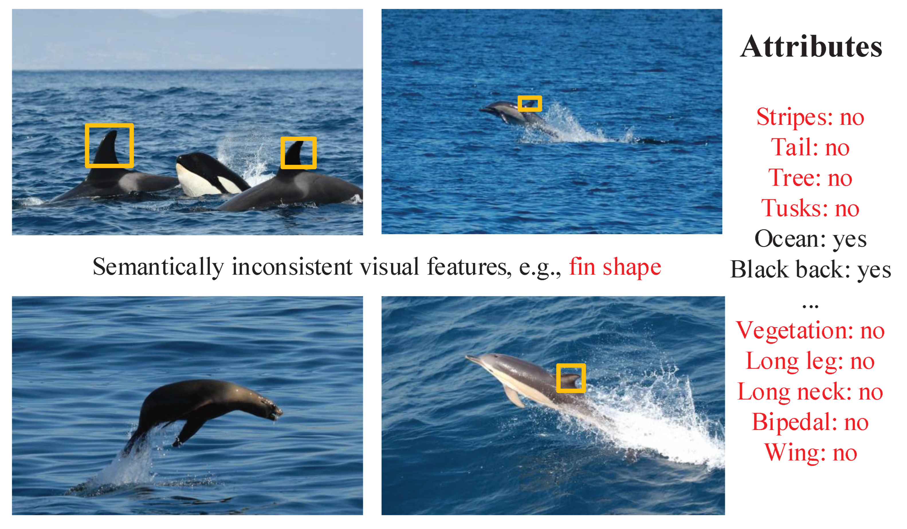
Both of these strategies align visual-semantic features through either generative or embedding methods, tackling the challenges inherent in ZSL. However, they introduce a new challenge: they often overlook the potential inconsistency in the visual-semantic features to be aligned, as illustrated in
Figure 1. Most GZSL methods overlook these inconsistent visual-semantic features and forcibly align them, potentially introducing biases in visual-semantic feature alignment and undermining the recognition of unseen classes. Moreover, current GZSL approaches frequently employ pre-trained ImageNet models for extracting GZSL visual features and training generative models to synthesize visual features of unseen classes. However, the presence of cross-modal dataset bias [
19] implies that the extracted and synthesized visual features might lack refinement and could stray from the visual features necessary for ZSL tasks, thereby worsening the problem of visual-semantic feature inconsistency.
We think that extracting and synthesizing refined visual features to enhance the semantic consistency of visual features, and segregating semantic-consistent visual features and visually consistent non-redundant semantic features from raw visual-semantic features to bolster the consistency of visual-semantic features, can alleviate the aforementioned issues. Hence, this paper proposes a GZSL framework that enhances the consistency of visual-semantic features using self-distillation and disentanglement network. Specifically, We first devised a self-distillation module that leverages self-distillation technology to augment both the feature extraction model and the generative model in the context of generative GZSL. This enables them to concurrently acquire refined mid-layer features and soft label knowledge from the auxiliary self-teacher network, thereby stimulating the model to extract and synthesize refined visual features. Additionally, we devise a disentanglement network applied to the visual-semantic modality. For instance, in the visual modality, the visual disentanglement encoder projects visual features into and . To ensure the consistency of with semantic features, visual-semantic features are cross-reconstructed, and a semantic relationship matching method is employed to calculate the compatibility score between and semantic information to guide the learning of . Furthermore, a latent representation independent method is applied to enforce the independence between and . Ultimately, the disentanglement network attains consistent visual-semantic features, which are amalgamated to jointly train a GZSL classifier.
In summary, the contributions of this paper are as follows:
We identified that most models typically do not handle visually-semantic inconsistent features and directly align them, which may lead to alignment bias. We propose an approach to enhance the consistency of visually-semantic features by refining visual features and disentangling original visually-semantic features.
We designed a self-distillation embedding module, which generates soft labels through an auxiliary self-teacher network and employs soft label distillation and feature map distillation methods to refine original visual features of seen classes and synthesized visual features of unseen classes from the generator, thereby enhancing the semantic consistency of visual features.
We proposed a disentanglement network, which encodes visually-semantic features into latent representations and promotes visually-semantic consistent features to be separated from original features through semantic relation matching and latent representation independence methods, significantly enhancing the consistency of visually-semantic features.
Extensive experiments on four GZSL benchmark datasets demonstrate that our model can separate refined visually-semantic features with consistency from original visually-semantic features, thereby alleviating alignment bias caused by visually-semantic inconsistency and improving the performance of GZSL models.
2. Related Work
2.1. Generative-Based Generalized Zero-Shot Learning
In recent years, numerous studies have employed generative models to bolster the efficacy of GZSL tasks. GANs or VAEs are commonly utilized in generative GZSL to synthesize visual features for unseen classes. These synthesized visual features for unseen classes are subsequently integrated with original visual features for seen classes to train classifiers. For example, Narayan et al. [
32] employed VAEs and GANs to refine the quality of synthesized visual features for unseen classes. They introduced a feedback module to regulate the generator’s output, effectively diminishing ambiguity between classes. Zhang et al. [
3] combined generative and embedding-based models by projecting real and synthesized samples onto an embedding space for classification, establishing a hybrid ZSL framework that effectively addresses data imbalance issues. Li et al. [
2] proposed an innovative approach that integrates a Transformers model with VAE and GAN, capitalizing on the rich data representation from VAE and the diversity of data generated by GAN to mitigate dataset diversity bias, while utilizing Transformers to enhance semantic consistency. DGCNet [
4] introduced a Dual Uncertainty Guided Cycle-Consistent Network, which examines the relationship between visual and semantic features through a cycle-consistent embedding framework and dual uncertainty-aware modules, effectively addressing alignment shift problems and enhancing model discriminability and adaptability. However, these methods often ignore the existence of semantically inconsistent visual features and redundant semantic attributes in the original visual-semantic features, which may affect the correct alignment of visual-semantic features. Instead, by first decoupling visually-semantic consistent features before alignment, we have improved the model’s accuracy.
2.2. Knowledge Distillation
Knowledge distillation [
18] serves as a model compression technique, aiming to reduce the size and computational complexity of a model by transferring knowledge from a complex neural network (referred to as the teacher network) to a smaller neural network (referred to as the student network) . Initially, the concept of knowledge distillation emerged by encouraging the student network to imitate the output log-likelihood of the teacher network [
41]. Subsequ ent research introduced intermediate layer distillation methods, enabling the student network to acquire knowledge from the convolutional layers of the teacher network with feature map-level locality [
5,
6,
7,
8], or from the penultimate layer of the teacher network [
9,
10,
11,
12,
13]. However, these methods necessitate pre-training a complex model as the teacher network, a process consuming substantial time and resources. Some recent studies have proposed self-knowledge distillation [
45,
46], enhancing the training of the student network by leveraging its own knowledge without requiring an additional teacher network. For instance, Zhang et al. [
42] segmented the network into several parts and compressed deep-layer knowledge into shallow layers. DLB [
43] utilizes instant soft targets generated in the training process of the previous iteration for distillation, achieving performance improvement without altering the model structure. FRSKD [
44] introduces an auxiliary self-teacher network to refine knowledge transfer to the student’s classifier network, capable of performing self-knowledge distillation using both soft labels and feature map distillation. This paper adopts the concept proposed by FRSKD to construct a self-distillation embedding module, aiming to refine the original seen visual features and the unseen visual features synthesized by the generator.
3. Materials and Methods
3.1. Problem Definition
In GZSL, the dataset comprises visual features X, semantic attributes C, and labels Y, which can be divided into seen classes S and unseen classes U. Specifically, the visual feature set is defined as , and the corresponding label set is represented as , where and are disjoint sets. Semantic attributes are defined as . Visual features and are defined as the ith visual feature, where and . The corresponding labels for seen and unseen classes are denoted as and , while and represent the ith semantic feature, where and . Thus, the training dataset is defined as , and the testing dataset is defined as . The objective of GZSL is to learn a classifier .
3.2. Overall Framework
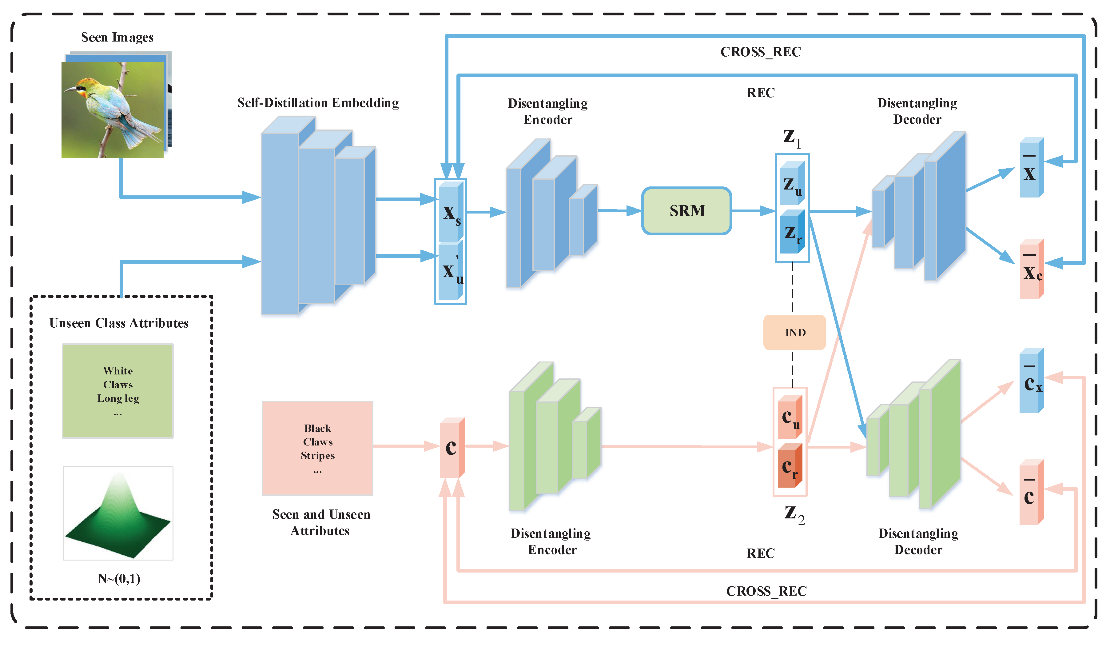
The SDDN architecture primarily comprises two key modules, as depicted in
Figure 2. The first module, known as the self-distillation embedding module, utilizes feature fusion techniques and an auxiliary self-teacher network to transfer refined visual features to the student network. It then employs both soft label distillation and feature map distillation to facilitate the generation of refined features by the generative model, thereby enhancing the consistency of visual-semantic features. The second module, referred to as the disentanglement network, employs semantic relationship matching (SRM) method and latent representation independent (IND) method to guide the visual-semantic disentanglement autoencoder in decoupling semantic-consistent visual features and non-redundant semantic features, further strengthening the consistency of visual-semantic features.
3.3. Self-Distillation Embedding Module
In order to refine the seen visual features extracted by the pre-trained ResNet101 [
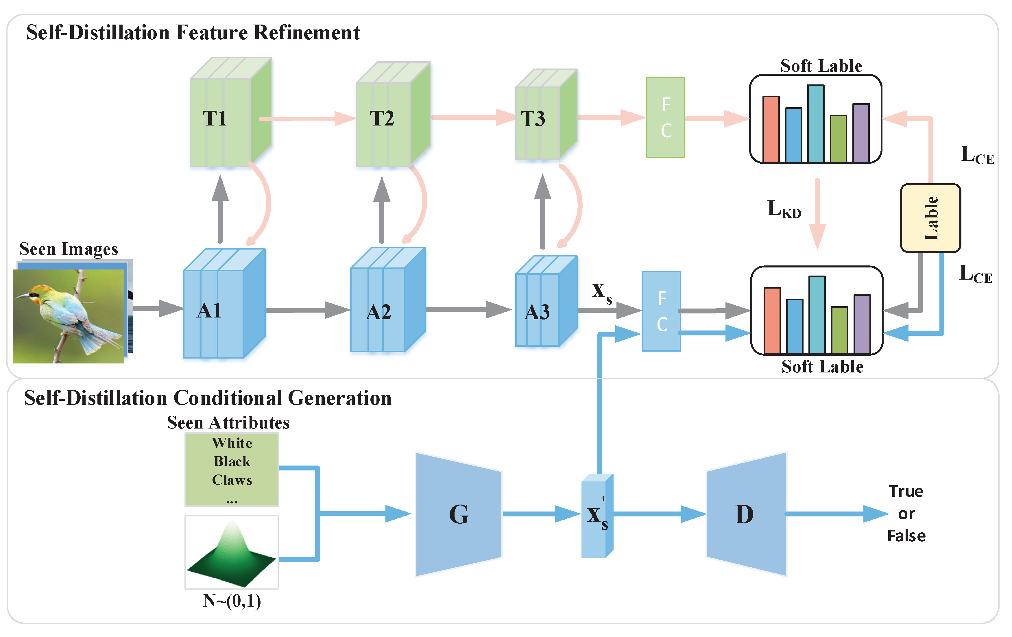
16] and the unseen visual features synthesized by the generator, thereby improving their semantic consistency. We designed a self-distillation embedding (SDE) module using self-distillation technology, as shown in
Figure 3. Firstly, this module establishes an auxiliary self-teacher network, employing specialized feature fusion methods to acquire refined feature maps. Subsequently, it utilizes soft label distillation and feature map distillation to assist the generation model and pre-trained ResNet101 in acquiring knowledge from feature maps and soft labels, refining the extracted and synthesized visual features.
3.3.1. Auxiliary Self-Teacher Network
To refine the visual features extracted by the pre-trained ResNet101 [
16] and pass them into generation model, we devised an auxiliary self-teacher network
T (illustrated in green in
Figure 3) based on the architecture proposed by Ji et al. [
44], comprising ResNet101, lateral convolutional layers, and feature fusion methods. The auxiliary self-teacher network employs top-down and bottom-up feature fusion to generate refined intermediate feature maps
and produces soft labels
at the final layer. Deep neural networks excel at learning representations at various levels; hence, outputs from intermediate and output layers can both contribute to training the student network. In our methodology, we employ ResNet101 (depicted in blue in
Figure 3) as the student network
A, enriching the visual features extracted by ResNet101 with soft labels
from the output of the self-teacher network and refined feature maps
from the intermediate layers. The formula for generating
in the auxiliary self-teacher network is defined as follows:
Here,
T is the temperature parameter (Hinton et al., 2015), typically set to 1. Higher values of
T result in softer class probability distributions. The student network learns from
through KL divergence, expressed as:
Here,
denotes the classifier of the student network. The student network learns refined intermediate layer features
through the loss function
, defined as:
Where
represents the channel pooling function. Additionally, class predictions are made on the enhanced visual features, and the cross-entropy loss between the prediction results and the true labels is minimized to ensure the accuracy of the enhanced visual features. Finally, the process of refining visual features through the self-learning network can be formalized as:
3.3.2. Self-Distillation Conditional Generation Module
The Self-Distillation Conditional Generation (SDCG) module aims to train the generator using soft labels and refined visual features generated by the auxiliary self-teacher network, thereby enabling the generator to synthesize refined visual features of unseen classes. The SDCG module employs a conditional generative adversarial network as the generator, utilizing Gaussian noise with a mean of 0 and standard deviation of 1 (
), and semantic descriptors of seen classes
as conditions to synthesize training features (
). Next, the synthesized
is input to the trained student network classifier to derive
. The objective is to minimize the loss between
and the soft labels
, ensuring that
remains consistent with the real visual features extracted by the auxiliary self-teacher network. The loss function is as follows:
Simultaneously, to ensure the accuracy of the synthesized visual features, the cross-entropy loss between
and the real labels
is computed. Additionally, the discriminator
D is employed to distinguish between real seen class samples
and synthesized seen class samples
.
Here,
, and
represents the penalty coefficient. The loss function for the SDCG module is as follows:
Finally, the overall loss of the SDE module is
3.4. Disentanglement Network
To further bolster the consistency of visual-semantic features, we propose a disentanglement network. This network utilizes a semantic relation matching method and an independent latent representation method to guide the visual-semantic disentangled autoencoder in separating visually consistent features and non-redundant semantic features from the original data. Furthermore, it aligns these features using a cross-reconstruction method to further strengthen their consistency.
3.4.1. Visual-Semantic Disentangled Autoencoder
The Visual-Semantic Disentangled Autoencoder (VSDA) comprises two parallel variational autoencoders dedicated to processing visual and semantic modalities separately. Each variational autoencoder includes a disentangled encoder and decoder. The disentangled encoder maps the feature space to the latent space, while the decoder maps the latent space back to the feature space. By optimizing the KL divergence loss between the latent variable distribution and the predefined prior distribution, the VSDA can acquire an effective latent space representation. The KL divergence loss for the VSDA is expressed as:
Define visual features
, where
represents seen visual features, and
denotes synthetic unseen visual features. Visual feature
x and semantic feature
c are encoded into latent representations
and
. Here,
and
represent the dimensions of semantically consistent visual features and non-redundant semantic features, respectively, while
and
denote the opposite. This process can be expressed as:
To mitigate information loss in visual and semantic modalities, a disentangled decoder is employed to reconstruct the latent representations
and
back to the original data and minimize their losses.
is reconstructed into visual features
through the visual unwrapping decoder
, and
is reconstructed into semantic features
. Their reconstruction loss is computed as follows:
Simultaneously, to enable the model to learn the association between visual and semantic features and reduce the deviation between modalities, cross-modal cross-reconstruction is designed. This involves using the semantic disentanglement decoder
to reconstruct the visual latent representation
and using the visual disentanglement decoder
to reconstruct the semantic latent representation
. This process can be expressed as:
Here, the mean square error (MSE) is utilized to calculate the reconstruction loss between the original visual features and the reconstructed features. Finally, the overall loss of the VSDA is:
3.4.2. Semantic Relation Matching
To disentangle the semantically consistent latent representation
and the semantically inconsistent latent representation
from the original visual space, we adopt the Relation Network (RN) [
22] to maximize the Compatibility Score (CS) between the latent representation
and the corresponding semantic embedding
c to make
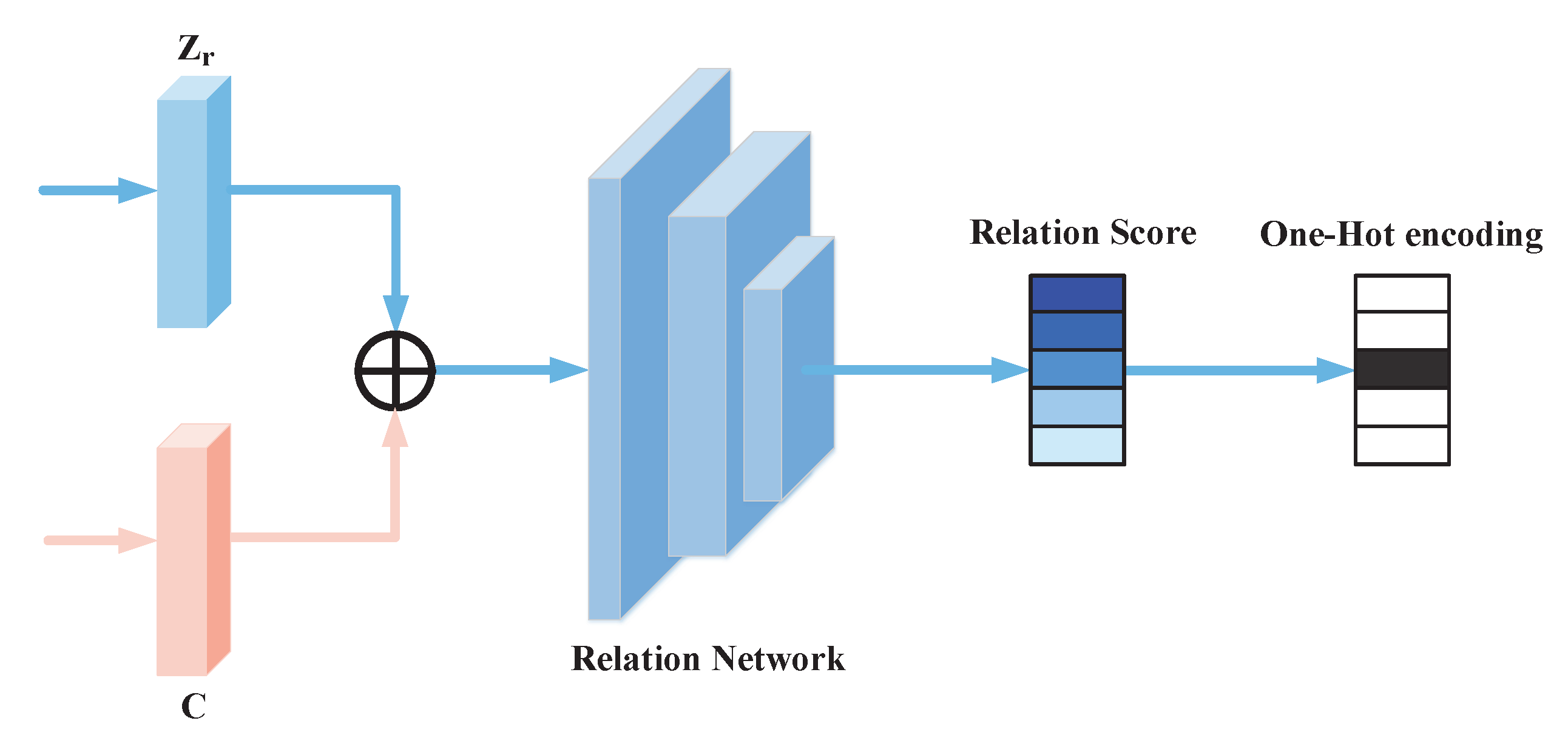
become semantically consistent. The model structure is shown in
Figure 4. The reason why the Relation Network is chosen as the semantic relation matching method here is that the Relation Network can calculate the distance between two samples by building a neural network, thereby measuring the degree of matching between them. The advantage of RN is that it can learn feature embeddings as well as nonlinear metric functions, which capture the similarities between features better than other metric methods. We use RN to concatenate
and its unique corresponding semantic embedding
c and input it into the relation network
R. The score for successful matching is 1, and the score for failed matching is 0. The formula of this process can be expressed as:
Here, t and b respectively represent the tth semantically consistent representation and the bth unique semantic embedding in the training batch, and represent the class labels of and respectively.
Figure 4.
Architecture of semantic relational matching model.
Figure 4.
Architecture of semantic relational matching model.
The relation network uses a Sigmoid activation function to constrain the relation score of each pair of outputs between 0 and 1. The loss function for optimizing
can be expressed as:
Here, B represents the size of the training batch, and n represents the number of corresponding unique semantic embeddings in the training batch. In each training batch, calculate the mean square error between the output of the relationship score of each pair and and the ground truth, optimized by the mean square error.This loss ensures that the model disentangle a semantically consistent latent representation .
3.4.3. Independence Between Latent Representations
During the encoding process, we anticipate the latent representation
in the visual modality to encompass visually consistent latent representations
with semantics and semantically unrelated latent representations
. Similarly, we expect the latent representation
in the semantic modality to include visually consistent latent representations
and visually unrelated latent representations
. This is crucial for segregating visually-semantic consistent features from the original features. Therefore, we devised a latent representation independence method to foster the segregation of visually-semantic consistent features and visually-semantic unrelated features in the visual-semantic modality. From a probabilistic perspective,
and
can be regarded as originating from different conditional distributions in the visual modality, while
and
can be considered to come from different conditional distributions in the semantic modality:
where
and
are distributions for
and
respectively, and
and
are distributions for
and
respectively. Thus, their overall independence
can be expressed as:
where
is the joint conditional probability of
and
, and similarly for the semantic modality. Taking the visual modality as an example, suppose that when
,
and
are dependent, denoted as
. While when
,
and
are independent, denoted as
. Therefore,
can be represented as:
We introduce a discriminator
to approximate
, thus
can be approximated by the following formula:
During the training of the discriminator, we randomly shuffle
and
in each training batch, then concatenate them to obtain
. Finally, the loss of the discriminator on the visual modality and the semantic modality is given by:
In summary, the total loss of our SDDN framework is formulated as:
3.5. Classification
When training the classifier, the seen visual features
, refined by the auxiliary self-teacher network, and the synthesized unseen visual features
from the SDCG module are combined into
. Next,
x is processed by the trained visual disentangling encoder to yield both semantically consistent latent representation
and semantically irrelevant latent representation
. Similarly, the semantic attribute set
c for both seen and unseen classes is fed into the trained semantic disentangling encoder, producing visually consistent latent representation
and visually irrelevant latent representation
. Subsequently, these representations
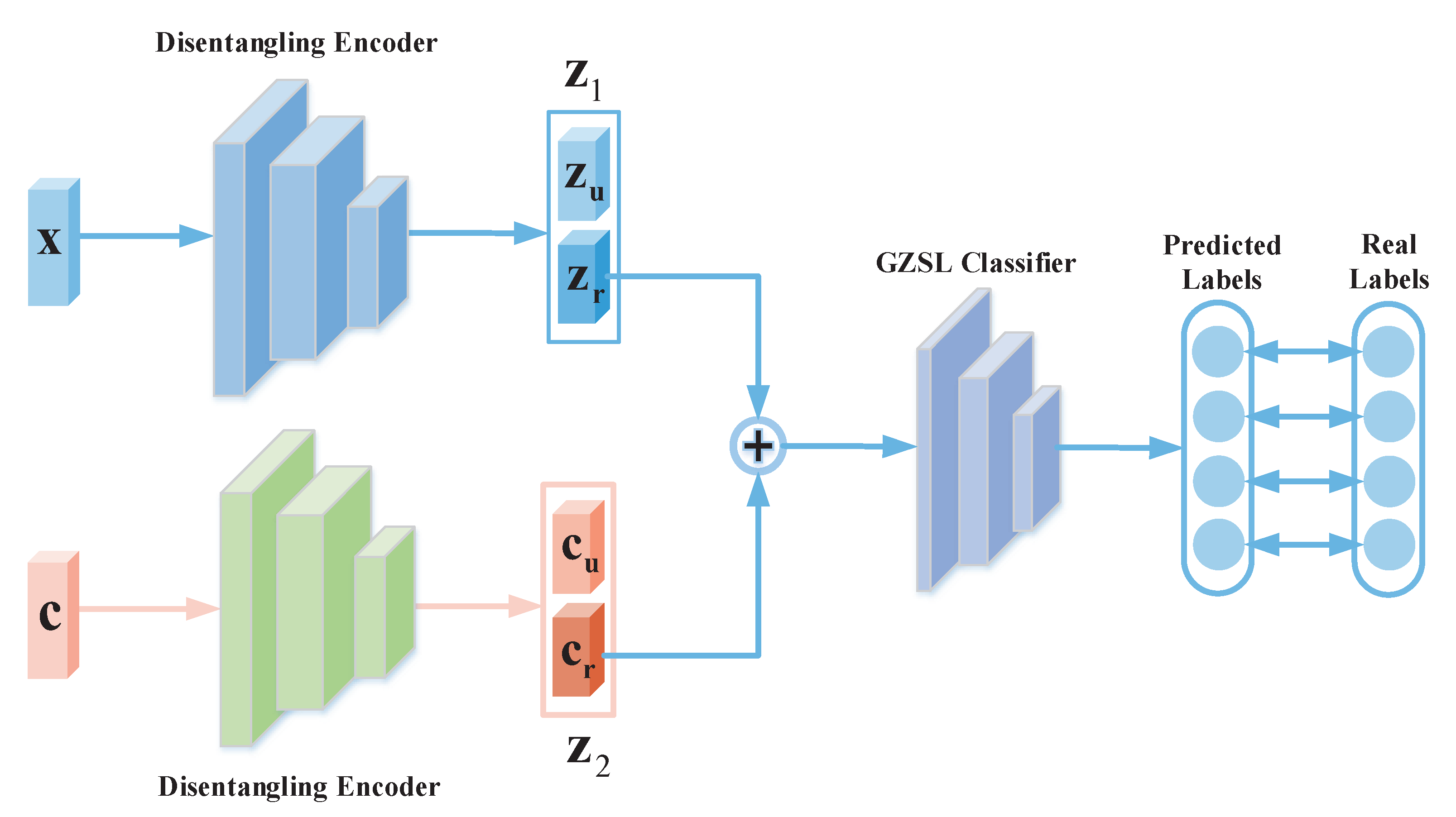
and
are fused and input into a softmax-based GZSL classifier for category prediction. Finally, the training concludes by minimizing the loss between the real and predicted labels. The whole process is shown in
Figure 5.
4. Experiments
4.1. Datasets
We conducted comprehensive tests on four publicly available benchmark datasets: Caltech-UCSD Birds-200-2011 (CUB) [
39], Animals with Attributes2 (AWA2) [
37], SUN Attribute Dataset (SUN) [
38], and Oxford Flowers (FLO) [
40]. All datasets and their statistics are summarized in
Table 1. CUB is a fine-grained dataset comprising 11,788 images from 200 different bird species, with 150 seen classes and 50 unseen classes. Each image in CUB is annotated with 312 dimensions of attributes. FLO is another fine-grained dataset consisting of flower images, containing 8,189 images across 102 classes, including 82 seen classes and 20 unseen classes. The annotation attributes in FLO have 1,024 dimensions. SUN is a fine-grained image dataset featuring various scenes, with 14,340 images covering 717 classes (645 seen classes and 72 unseen classes). Each scene in SUN is associated with 102-dimensional attributes describing its characteristics, such as lighting conditions, weather conditions, and terrain. AWA2 is a coarse-grained dataset with 37,322 animal images across 50 classes (10 seen classes and 40 unseen classes), covering a wide range of animals, including mammals, birds, and reptiles. Each image in AWA2 is labeled with attributes of dimension 85.
4.2. Evaluation Protocol
During testing, the accuracy is assessed on the test sets for both seen classes (S) and unseen classes (U). Here, U represents the average accuracy for each class on test images of unseen classes, indicating the model’s ability to classify samples from previously unseen classes. S represents the average accuracy for each class on test images of seen classes, reflecting the model’s ability to classify samples from seen classes. H (defined as ) represents the harmonic mean of S and U, serving as an evaluation metric for the performance of GZSL classification.
4.3. Implementation Details
SDDN mainly consists of a SDE module and a disentanglement network. The SDE module mainly consists of a student network, a self-teacher network, a generator and a discriminator. The student network is a ResNet101 model pre-trained on ImageNet and is used to extract visual features with a dimension of 2048. The self-teacher network is composed of the student network itself and the feature fusion method. In addition, the generator is implemented using a multi-layer perceptron with a hidden layer dimension of 2048, and the discriminator is implemented using a fully connected layer and activation function. The disentanglement network consists of an encoder, a decoder, a discriminator and a semantic relationship matching model. Both the encoder and decoder are multi-layer perceptrons with a single hidden layer and 2048 hidden units. The semantic relationship matching model consists of two fully connected layers activated with Smooth Maximum Unit (SMU) [
47] activation function and Sigmiod function respectively. The discriminator is implemented using a fully connected layer and SMU activation function.
The hardware environment used by SDDN is Intel i7-10700K CPU, RTX A5000 32GB GPU; the software environment is Ubuntu 20.04 LTS operating system, cuda 11.4.0, and cudnn 8.2.4. SDDN is implemented in PyTorch 1.10.1. The ADAM optimizer is used to optimize the parameters of each module. The learning rate of the Adam optimizer is set to , and . The batch size is 64. The loss weight of the semantic relation matching method, the loss weight of the latent representation independence method and the weight of the visual-semantic discriminator are set between 0.1-25.
4.3.1. Comparing with the State-of-the-Arts
To validate the effectiveness of our proposed SDDN model, we computed the seen class accuracy rate S, unseen class accuracy rate U, and their harmonic mean H on the aforementioned four datasets. We compared them with 15 state-of-the-art models, and the comparison results are shown in
Table 2. These 15 models are categorized into methods based on generative models and methods not based on generative models. Generative-based methods typically utilize techniques such as GANs or VAEs to generate synthetic unseen class data to augment the training dataset. These synthetic data can be used to train models in ZSL to improve their generalization capability to unseen classes. Non-generative-based methods, on the other hand, do not rely on generating synthetic data but achieve generalization to unseen classes through techniques such as feature embedding and alignment of existing data. Our method belongs to the generative-based methods.
From the comparison results in the table, firstly, our SDDN achieved the highest accuracy on U, S, and H on the FLO dataset, surpassing all compared models. Specifically, we outperformed the second-best model by 2.3% in the H metric. There was a significant improvement in the U metric, where we led the second-best by 4%. In the S metric, we were ahead of the second-best by 0.3%. On the CUB dataset, we achieved the highest accuracy on the U metric, leading the second-best by 1.1%. Additionally, we obtained the second-best accuracy on both U and S metrics, leading the third-best by 6% and 1.9%, respectively. On the SUN dataset, we attained the highest accuracy on both S and H metrics, leading the second-best by 2% in the H metric and 1.4% in the S metric.
Overall, our performance was the best in the H metric on these three fine-grained datasets: FLO, CUB, and SUN, the best on U in FLO, and the best on S in both FLO and SUN. This indicates that the richer the information in the dataset, the more effectively our proposed method can capture it through self-distillation and disentanglement techniques, separating visually-semantic consistent features and aligning them effectivel.
5. Model Analysis
5.1. Ablation Study
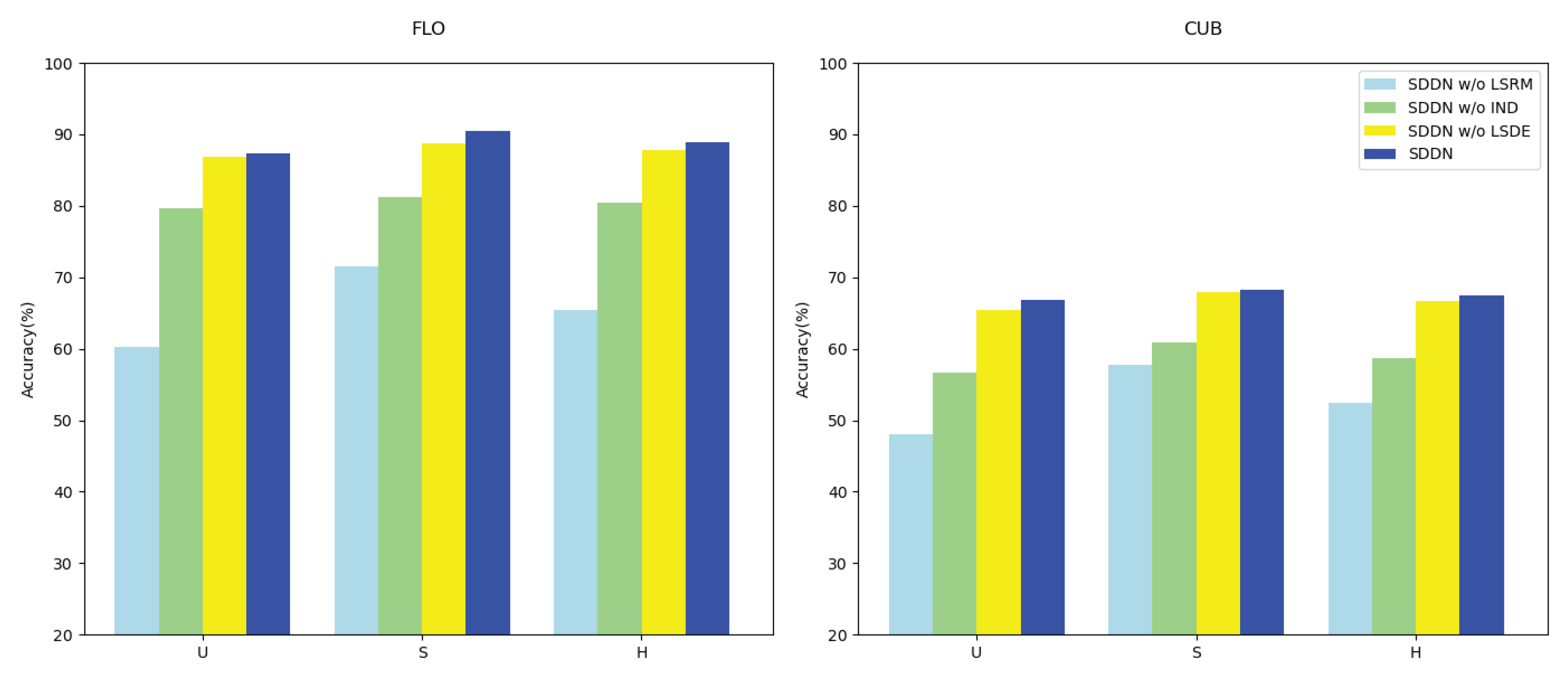
In our ablation study, we aim to isolate the key components of SDDN and assess their impact on GZSL. We remove the Semantic relation matching loss (LSRM) to evaluate the contribution of the Visual-Semantic Matching module to extracting semantically consistent visual features. Omitting the Independence score (IND) allows us to evaluate its contribution to further separating visually-semantic consistent features. Additionally, we exclude the loss of the self-distillation embedding module (LSDE) and then used the pre-trained ResNet101 and regular generator without employing the self-distillation technique. This evaluation helps assess the refinement effect of SDE on extracting and synthesizing visual features, while validating the effectiveness of the disentanglement network. Our ablation experiments were conducted on the FLO and CUB datasets, with the experimental results presented in
Table 3 and
Figure 6.
The results underscore the critical importance of the semantic relation matching module (LSRM), Independence score (IND), and self-distillation embedding module (LSDE) for the performance of SDDN. Firstly, LSRM is particularly crucial for visual-semantic feature alignment, as its removal leads to a significant decrease in the accuracy of seen classes (S), unseen classes (U), and the harmonic mean (H). Secondly, IND is essential for further separating visually-semantic consistent features from the original features, as its removal results in lower U, S, and H values. Additionally, LSDE helps refine the original visual features of seen classes and the synthesized features of unseen classes, as the model without LSDE performs lower in U, S, and H compared to the complete SDDN. Furthermore, when comparing
Table 1, it is found that the model without SDE still achieves the highest H score on FLO and CUB, indicating the effectiveness of the disentanglement network. Finally, the complete SDDN model demonstrates superior performance across all metrics, proving its effectiveness in GZSL.
5.2. Hyper-Parameter Analysis
In this study, the optimization objective of SDDN is determined by three critical hyperparameters: the coefficient of semantic relationship matching loss (
), the coefficient of independence of latent representations (
), and the coefficient of discriminator loss (
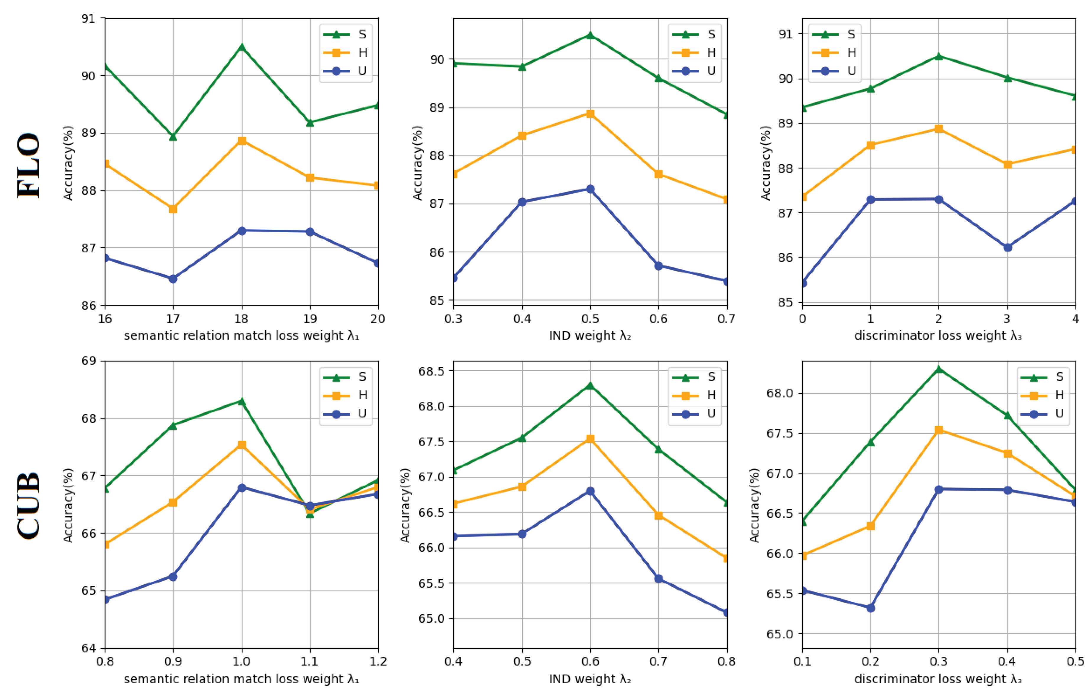
). To elucidate the influence of each hyperparameter on model performance, sensitivity analysis was conducted by varying the hyperparameter values in the experiments. Specifically,
was varied within the range of 0.3-20.0, while
and
were varied within the range of 0.1-3.0.
Figure 7 illustrates the significant impact of hyperparameter values
,
, and
on the experimental outcomes. Notably, when
is set to 18,
is set to 0.5, and
is set to 2, the model achieves its highest accuracy on the FLO dataset. Whereas, when
is set to 1,
is set to 0.6, and
is set to 0.3, the model achieves its highest accuracy on the CUB dataset. These observations underscore the substantial influence of hyperparameter weights on model accuracy, indicating the model’s high sensitivity to these hyperparameters. Based on these findings, we advocate for future experiments to focus on exploring the specific impact of minor fluctuations in these three hyperparameter values on accuracy. This systematic analysis of hyperparameters will contribute to a deeper comprehension of model behavior and offer valuable insights for optimizing model performance across diverse datasets.
5.3. Zero-Shot Retrieval Performance
To assess the practical application performance of our SDDN framework, we conducted zero-shot retrieval experiments comparing SDDN with two other state-of-the-art generative-based GZSL frameworks: DGGNet-db and DVAGAN. The experiment follows the zero-shot retrieval protocol in SDGZSL [
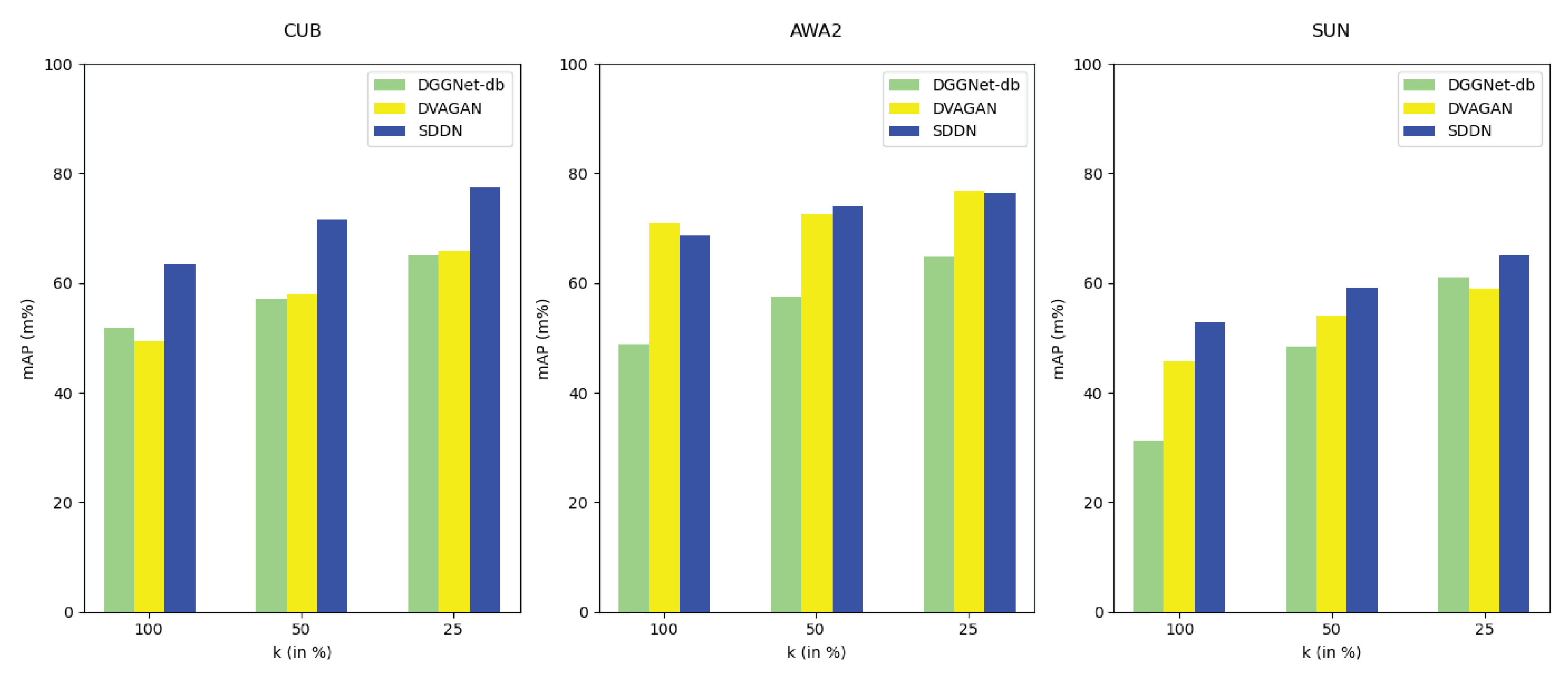
17]. In zero-shot retrieval experiments, we initially provide semantic features of unseen classes, followed by employing the generation modules of SDDN, DGGNet-db, and DVAGAN to synthesize a certain number of visual features for these unseen classes. Throughout this process, the average of the synthesized visual features for each category is computed as the retrieval feature. Subsequently, the cosine similarity between the retrieval features and the true features is calculated, and the true features are ranked in descending order based on this similarity. The performance of zero-shot image retrieval is evaluated using mean Average Precision (mAP). Experimental analyses are performed on three datasets: CUB, AWA2, and SUN. The results, illustrated in
Figure 8, compare SDDN, DGGNet-db, and DVAGAN in terms of zero-shot retrieval performance. The horizontal coordinates 100, 50, and 25 represent the proportions of unseen category images in the test dataset, being 100%, 50%, and 25%, respectively, while the vertical coordinate represents the average retrieval accuracy. Results indicate significantly higher zero-shot retrieval performance of the SDDN framework on the CUB and SUN datasets compared to DGGNet-db and DVAGAN. In the AWA2 dataset, we achieve the best performance when the proportion of unseen category images reaches 50%, and it remains close to the best performance when the proportion reaches 100%. These zero-shot retrieval performance tests on the three datasets further validate the effectiveness of the model.
6. Conclusion
In this paper, we propose a generalized zero-shot learning framework that utilizes self-distillation and disentanglement network to enhance visual-semantic feature consistency. Initially, for improving the semantic consistency of visual features, we develop a self-distillation embedding framework integrating self-distillation techniques with a conditional generator to prompt the synthesis of refined visual features. Subsequently, to further promote visual-semantic feature consistency, we design a disentanglement network. We use semantic relation matching networks and latent representation independence methods to facilitate the separation of visually semantically consistent features from inconsistent features. Additionally, we devise a cross-reconstruction method to align visual and semantic features within a visual-semantic common space, thereby enhancing the semantic consistency of visual-semantic features. Extensive experiments are conducted on four widely used benchmark datasets in GZSL. We compare SDNN with current state-of-the-art methods, thereby demonstrating the superiority of the proposed SDNN framework. In future work, we intend to optimize the model further and apply it in the field of medical diagnostics to assist in identifying new disease patterns.
Author Contributions
Responsible for proposing research ideas,modeling frameworks, content planning, guidance,and full-text revisions: X.L.;Responsible for literature research, research methodology, experimental design, thesis writing, and full text revision: C.W.;Responsible for lab instruction,guidelines,and full text revisions:G.Y. and CH.W.;Responsible for providing guidance, revising,and reviewing full texts:,Y.L.,J.L. and Z.Z.All authors have read and agreed to the published version ofthe manuscript.
Funding
This work was supported by National Key Research and Development Program of China (2020AAA0109700), National Science and Technology Major Project (2020AAA0109703), National Natural Science Foundation of China (62076167, U23B2029), the Key Scientific Research Project of Higher Education Institutions in Henan Province (24A520058, 24A520060) and Postgraduate Education Reform and Quality Improvement Project of Henan Province (YJS2024AL053).
Data Availability Statement
Data are contained within the article.
Conflicts of Interest
The authors declare that they have no conflict of interest.
References
- Z. Wang, Y. Hao, T. Mu, O. Li, S. Wang, and X. He, “Bi-directional distribution alignment for transductive zero-shot learning,” 2023.
- N. Li, J. Chen, N. Fu, W. Xiao, T. Ye, C. Gao, and P. Zhang, “Leveraging dual variational autoencoders and generative adversarial networks for enhanced multimodal interaction in zero-shot learning,” Electronics, vol. 13, no. 3, p. 539, 2024. [CrossRef]
- M. Zhang, X. Wang, Y. Shi, S. Ren, and W. Wang, “Zero-shot learning with joint generative adversarial networks,” Electronics, vol. 12, no. 10, p. 2308, 2023. [CrossRef]
- Y. Zhang, Y. Tian, S. Zhang, and Y. Huang, “Dual-uncertainty guided cycle-consistent network for zero-shot learning,” IEEE Transactions on Circuits and Systems for Video Technology, 2023. [CrossRef]
- S. Zagoruyko and N. Komodakis, “Paying more attention to attention: Improving the performance of convolutional neural networks via attention transfer,” 2017.
- J. Kim, S. Park, and N. Kwak, “Paraphrasing complex network: Network compression via factor transfer,” 2020.
- J. Yim, D. Joo, J. Bae, and J. Kim, “A gift from knowledge distillation: Fast optimization, network minimization and transfer learning,” in 2017 IEEE Conference on Computer Vision and Pattern Recognition (CVPR), 2017, pp. 7130–7138. [CrossRef]
- A. Koratana, D. Kang, P. Bailis, and M. Zaharia, “Lit: Learned intermediate representation training for model compression,” in International Conference on Machine Learning. PMLR, 2019, pp. 3509–3518.
- F. Tung and G. Mori, “Similarity-preserving knowledge distillation,” 2019.
- B. Peng, X. Jin, J. Liu, S. Zhou, Y. Wu, Y. Liu, D. Li, and Z. Zhang, “Correlation congruence for knowledge distillation,” 2019.
- Y. Tian, D. Krishnan, and P. Isola, “Contrastive representation distillation,” 2022.
- Y. Liu, J. Cao, B. Li, C. Yuan, W. Hu, Y. Li, and Y. Duan, “Knowledge distillation via instance relationship graph,” in Proceedings of the IEEE/CVF Conference on Computer Vision and Pattern Recognition (CVPR), June 2019. [CrossRef]
- W. Park, D. Kim, Y. Lu, and M. Cho, “Relational knowledge distillation,” in Proceedings of the IEEE/CVF Conference on Computer Vision and Pattern Recognition (CVPR), June 2019. [CrossRef]
- K. Sun, X. Zhao, H. Huang, Y. Yan, and H. Zhang, “Boosting generalized zero-shot learning with category-specific filters,” Journal of Intelligent & Fuzzy Systems, no. Preprint, pp. 1–14.
- H. Jiang, R. Wang, S. Shan, and X. Chen, “Transferable contrastive network for generalized zero-shot learning,” 2019.
- K. He, X. Zhang, S. Ren, and J. Sun, “Deep residual learning for image recognition,” 2015.
- Z. Chen, Y. Luo, R. Qiu, S. Wang, Z. Huang, J. Li, and Z. Zhang, “Semantics disentangling for generalized zero-shot learning,” 2021.
- Z. Han, Z. Fu, S. Chen, and J. Yang, “Contrastive embedding for generalized zero-shot learning,” 2021.
- S. Chen, W. Wang, B. Xia, Q. Peng, X. You, F. Zheng, and L. Shao, “Free: Feature refinement for generalized zero-shot learning,” 2021.
- X. Li, Z. Xu, K.-J. Wei, and C. Deng, “Generalized zero-shot learning via disentangled representation,” in AAAI Conference on Artificial Intelligence, 2021. [CrossRef]
- B. Tong, C. Wang, M. Klinkigt, Y. Kobayashi, and Y. Nonaka, “Hierarchical disentanglement of discriminative latent features for zero-shot learning,” in Proceedings of the IEEE/CVF conference on computer vision and pattern recognition, 2019, pp. 11 467–11 476. [CrossRef]
- F. Sung, Y. Yang, L. Zhang, T. Xiang, P. H. S. Torr, and T. M. Hospedales, “Learning to compare: Relation network for few-shot learning,” 2018.
- S. Min, H. Yao, H. Xie, C. Wang, Z.-J. Zha, and Y. Zhang, “Domain-aware visual bias eliminating for generalized zero-shot learning,” 2020.
- G.-S. Xie, L. Liu, F. Zhu, F. Zhao, Z. Zhang, Y. Yao, J. Qin, and L. Shao, “Region graph embedding network for zero-shot learning,” in Computer Vision–ECCV 2020: 16th European Conference, Glasgow, UK, August 23–28, 2020, Proceedings, Part IV 16. Springer, 2020, pp. 562–580. [CrossRef]
- Y. Liu, L. Zhou, X. Bai, Y. Huang, L. Gu, J. Zhou, and T. Harada, “Goal-oriented gaze estimation for zero-shot learning,” 2021.
- C. Wang, S. Min, X. Chen, X. Sun, and H. Li, “Dual progressive prototype network for generalized zero-shot learning,” 2021.
- C. Wang, X. Chen, S. Min, X. Sun, and H. Li, “Task-independent knowledge makes for transferable representations for generalized zero-shot learning,” 2021.
- Y. Xian, S. Sharma, B. Schiele, and Z. Akata, “f-vaegan-d2: A feature generating framework for any-shot learning,” 2019.
- Z. Chen, J. Li, Y. Luo, Z. Huang, and Y. Yang, “Canzsl: Cycle-consistent adversarial networks for zero-shot learning from natural language,” 2019.
- J. Li, M. Jin, K. Lu, Z. Ding, L. Zhu, and Z. Huang, “Leveraging the invariant side of generative zero-shot learning,” 2019.
- J. Kim, K. Shim, and B. Shim, “Semantic feature extraction for generalized zero-shot learning,” 2021.
- S. Narayan, A. Gupta, F. S. Khan, C. G. M. Snoek, and L. Shao, “Latent embedding feedback and discriminative features for zero-shot classification,” 2020.
- L. Feng and C. Zhao, “Transfer increment for generalized zero-shot learning,” IEEE Transactions on Neural Networks and Learning Systems, vol. 32, pp. 2506–2520, 2020. [CrossRef]
- Y. Feng, X. Huang, P. Yang, J. Yu, and J. Sang, “Non-generative generalized zero-shot learning via task-correlated disentanglement and controllable samples synthesis,” in Proceedings of the IEEE/CVF Conference on Computer Vision and Pattern Recognition, 2022, pp. 9346–9355. 10.1109/CVPR52688.2022.0091310.1109/CVPR52688.2022.00913.
- G. Kwon and G. AlRegib, “A gating model for bias calibration in generalized zero-shot learning,” 2022.
- X. Kong, Z. Gao, X. Li, M. Hong, J. Liu, C. Wang, Y. Xie, and Y. Qu, “En-compactness: Self-distillation embedding & contrastive generation for generalized zero-shot learning,” in Proceedings of the IEEE/CVF Conference on Computer Vision and Pattern Recognition, 2022, pp. 9306–9315.
- Y. Xian, C. H. Lampert, B. Schiele, and Z. Akata, “Zero-shot learning – a comprehensive evaluation of the good, the bad and the ugly,” 2020.
- G. Patterson and J. Hays, “Sun attribute database: Discovering, annotating, and recognizing scene attributes,” in 2012 IEEE Conference on Computer Vision and Pattern Recognition, 2012, pp. 2751–2758. [CrossRef]
- P. Welinder, S. Branson, T. Mita, C. Wah, F. Schroff, S. Belongie, and P. Perona, “Caltech-ucsd birds 200,” 2010.
- M.-E. Nilsback and A. Zisserman, “Automated flower classification over a large number of classes,” in 2008 Sixth Indian conference on computer vision, graphics & image processing. IEEE, 2008, pp. 722–729. [CrossRef]
- G. Hinton, O. Vinyals, and J. Dean, “Distilling the knowledge in a neural network,” arXiv preprint arXiv:1503.02531, 2015.
- L. Zhang, J. Song, A. Gao, J. Chen, C. Bao, and K. Ma, “Be your own teacher: Improve the performance of convolutional neural networks via self distillation,” in Proceedings of the IEEE/CVF international conference on computer vision, 2019, pp. 3713–3722. [CrossRef]
- Y. Shen, L. Xu, Y. Yang, Y. Li, and Y. Guo, “Self-distillation from the last mini-batch for consistency regularization,” in Proceedings of the IEEE/CVF Conference on Computer Vision and Pattern Recognition, 2022, pp. 11 943–11 952.
- M. Ji, S. Shin, S. Hwang, G. Park, and I.-C. Moon, “Refine myself by teaching myself: Feature refinement via self-knowledge distillation,” 2021.
- M. Caron, H. Touvron, I. Misra, H. Jégou, J. Mairal, P. Bojanowski, and A. Joulin, “Emerging properties in self-supervised vision transformers,” 2021.
- T.-B. Xu and C.-L. Liu, “Data-distortion guided self-distillation for deep neural networks,” Proceedings of the AAAI Conference on Artificial Intelligence, vol. 33, pp. 5565–5572, 07 2019. [CrossRef]
- K. Biswas, S. Kumar, S. Banerjee, and A. K. Pandey, “Smooth maximum unit: Smooth activation function for deep networks using smoothing maximum technique,” in Proceedings of the IEEE/CVF Conference on Computer Vision and Pattern Recognition, 2022, pp. 794–803. [CrossRef]
|
Disclaimer/Publisher’s Note: The statements, opinions and data contained in all publications are solely those of the individual author(s) and contributor(s) and not of MDPI and/or the editor(s). MDPI and/or the editor(s) disclaim responsibility for any injury to people or property resulting from any ideas, methods, instructions or products referred to in the content. |
© 2024 by the authors. Licensee MDPI, Basel, Switzerland. This article is an open access article distributed under the terms and conditions of the Creative Commons Attribution (CC BY) license (http://creativecommons.org/licenses/by/4.0/).
