
Submitted:
09 April 2024
Posted:
10 April 2024
You are already at the latest version
Abstract
Myanmar is located in the Indo-Burma biodiversity hotspot, but lacks understanding of the bio-diversity hotspots and protected areas within its borders. Climate change affects the effective-ness of protected areas and the potential distribution range of species. Based on Myanmar's re-gional characteristics, endangered status, and representativeness, this paper selects species and identifies biodiversity hotspots using the MaxEnt model. We studied the biodiversity within the terrestrial protected area network in Myanmar, as well as the potential for cross-boundary range shifts among protected areas under different climate scenarios. Species populations outside My-anmar's protected area network may not be able to find suitable habitats in the future, further exacerbating climate-related extinction risks. Additionally, some protected areas in Myanmar may not be fully utilizing their biodiversity representation potential, and with scientific spatial planning, Myanmar's protected areas could support a large number of species. In the context of continued warming, identifying new protected areas that encompass the future and current climatic niches of protected areas can increase the capacity for sustained biodiversity conservation. We hope that this study provides insights for increasing the effectiveness of Myanmar's protect-ed area network and emphasizes the urgency of coordinated protection of protected areas and biodiversity hotspots.
Keywords:
climate change
; protected area network
; biodiversity
; cross-boundary range shift
; Indo-Burma biodiversity hotspot
1. Introduction
1.1. Biodiversity Hotspot Areas and Protected Areas
Over the past century, the decline in global biodiversity has been more severe than at any other time in human history [1,2,3]. Some scholars believe that the world’s species are currently experiencing the sixth mass extinction driven by humans [4]. The habitats of global biodiversity hotspot areas are shrinking [5,6]. Additionally, the extinction risks among taxonomic groups vary across different geographical regions, with biodiversity conservation in tropical regions requiring particular attention [7,8]. Myanmar, located in the Indo-Burma biodiversity hotspot, serves as a critical link between the Sunda, Wallacea, and Philippine biodiversity hotspots [9,10]. Throughout history, the main threats to biodiversity conservation in Myanmar have included increasing population density, infrastructure development in forested areas, changes in land use [11], and large-scale exploitation of non-renewable natural resources [12]. Since 2010, Myanmar’s political system has become more democratic, and international political sanctions against the country have begun to ease, allowing a significant influx of commercial capital. Myanmar’s forests are increasingly threatened by commercial development for oil, palm, rubber, minerals, and timber [13,14,15,16], all of which are crucial issues for biodiversity conservation in Myanmar [14,17].
Identifying biodiversity hotspots and critical habitats for species is an effective approach to biodiversity conservation [18,19], and regional-scale reserve planning is also an important strategy for biodiversity conservation [20]. Increasing the coverage of protected areas is a target set by the Convention on Biological Diversity for biodiversity conservation [21]. However, due to limited funds and resources for biodiversity conservation management, many parts of the world are facing issues of inefficiency [22,23].
The effectiveness of protected area management can be evaluated through the distribution of indicator species. Starting from Rosenzweig’s classic works, ecological scholars have placed special emphasis on the study of species distribution [24,25,26], which has carried on into the field of biodiversity conservation [27,28]. Wildlife hunting in Southeast Asia has existed for thousands of years [29,30], providing raw materials for traditional medicine, pets, handicrafts, etc. [31,32,33], which may alter regional species composition [34]. Habitats are often affected by invasive species, resource exploitation, and other factors [35,36]. Hunting and habitat loss are the main reasons for the decline in large mammal populations in many protected areas in Myanmar [37], and illegal activities weaken the role of protected areas [38].
Furthermore, data on species distribution and abundance are crucial for identifying critical habitats and hotspots, but such data are often scarce and of low precision. In the face of climate change, biodiversity conservation efforts at the regional scale are challenged by changes in the geographical ranges of various species [42,43]. However, protected area boundaries often lack flexibility to respond to changes in habitat ranges due to cumbersome planning procedures. The overlap between species habitat ranges and protected area coverage is crucial for enhancing the effectiveness of reserve construction [44].
The speed of climate change describes the rate of change in climatic conditions across geographical spaces [45]. In areas with high topographic heterogeneity, climate gradients vary significantly, resulting in generally low rates of climate change [46]. This makes it easier for low-mobility species to adapt to climate change, which is one reason why many mountainous regions with high topographic heterogeneity often have rich and unique species [47]. Typically, endemic species have poor spatial dispersal abilities and are mostly confined to high-altitude areas, making them vulnerable to losing most of their suitable habitats during climate warming [48]. Weak dispersal abilities, combined with geographical barriers [49,50], and the degree of connectivity between protected areas limit this migration process [51]. Although topographic heterogeneity can buffer the impact of climate change on regional biodiversity, high endemism still makes these areas potential hotspots for biodiversity loss [52,53]. Therefore, these endemic hotspots urgently need protection planning that addresses climate change.
Classical species distribution models are often used to predict changes in the climatic suitability ranges of species [54]. However, the scarcity of distribution data for endemic species often reduces the predictive accuracy of these models [55]. Some scholars have attempted to assess the protective role of protected areas for these data-deficient species under climate change by comparing the climatic conditions within the protected areas with the overall climatic conditions in larger regions [56]. Since small heterogeneous landscapes contain more climatic variations than large homogeneous landscapes [57], the loss of climatic niches may strongly affect future intraspecific diversity, thereby reducing the potential for species to evolve and adapt to climate change [58].
1.2. The History of Protected Areas in Myanmar
Myanmar has a long history of protected areas [59]. In 1860, King Mindon Min established the first recorded protected area, Yadanabon Bemetaw. Later, King Theebaw issued a royal decree to establish protected areas [60] in non-Buddhist regions where slash-and-burn agriculture was practiced. The Buddhist tradition of establishing hunting-free sacred sites has continued to the present day, and in Myanmar’s history, monks were sometimes appointed as protected area administrators [59]. Myanmar’s Wildlife Protection Act of 1936 prohibited hunting within 200 yards of Buddhist temples or religious buildings [61].
British colonizers, in order to secure their interests in Myanmar during the late 19th century, opened reserved forests to the Myanmar government for timber extraction [62,63]. Since then, there has been a decreasing trend in the species hunted [64], leading to the establishment of the Pidaung Sumatran rhinoceros reserve in 1918. Unlike the previously mentioned reserved forests, wildlife reserves prohibited any form of use by local residents [63]. The hunting administrators responsible for these areas had the primary responsibility of managing the forests for timber production [65]. The British colonizers’ practice of hiring Myanmar nationals at low salaries to serve as administrators in forest checkpoints created injustices and led to a large number of illegal activities [63]. In addition, there was no reserved forest space nearby Myanmar’s protected areas to serve as alternative conservation forests, resulting in the failure of the protected areas to protect wildlife [61].
In 1981, the Myanmar government, together with the United Nations Development Program (UNDP), initiated the Natural Conservation and National Park Project (NCNPP) [66]. The NCNPP developed conservation texts for Hlawga National Park (1982), Po Mountain Reserve (1983), Alaungdaw Katha National Park (1984), Chatthin Wildlife Reserve (1985), Inlay Wetland Wildlife Reserve (1994), Natmataung National Park (1995), and Hkakaborazi National Park (2003) [67]. During the NCNPP, the Forestry Department established the Natural and Wildlife Conservation Department (NWCD). The National Committee for Environmental Affairs (NCEA) was established in 1990 to formulate environmental policies and handle external liaison [63], although its authority and expertise still need to be improved [68].
Wildlife conservation and protected areas in Myanmar are part of broader land use issues under colonial rule, and therefore biodiversity conservation policies and legislation are based on European models [62].
Wildlife legislation in Myanmar preceded protected area policies [69]. Compared to other Southeast Asian countries, Myanmar’s conservation legislation is weaker in terms of comprehensiveness and enforceability [70], and Myanmar has not granted enforcement powers to protected area staff [71].
Although work plans for forest management in Myanmar have existed for many years [72,73], they rarely involve the management of wildlife or wildlife protected areas. Dissatisfied with the Forest Department’s ability to manage pristine wildlife protected areas, the Governor of Myanmar, Smith, suggested the establishment of a National Trust Fund composed of indigenous gentlemen from Myanmar [74]. Subsequently, it was proposed that wildlife conservation should be completely separated from forestry and an independent department should be established [61]. Thus, Myanmar’s protected areas are rooted in the country’s Buddhist history, but the modern policies and practices of the protected area system are the result of forest development activities during the British colonial period.
The lack of review procedures for protected area construction plans and the absence of scientific assessments of protected area effectiveness make it difficult to establish management priorities [75]. Cooperation between protected area managers and local communities can ensure the actual effectiveness of protected areas [76], with early examples of cooperation including “adopt-a-park programs” [77]. The Forest Resource Environment Development and Conservation Association (FREDA) and the Biodiversity and Nature Conservation Association (BANCA) have helped local communities engage in protected area practices [76]. The United Nations Development Program’s Community Development for Remote Townships (CDRT) project has mainly focused on Waimaw Township in Kachin State, Maungtaw Township in Kayah State, and Phalan Township in Chin State, gradually expanding its scope [76]. The project aims to increase the income of protected area residents through animal husbandry and loans [78]. These projects will need to be tailored to local conditions and gain the support of the local public [79] to facilitate adaptive management [80].
The ceasefire between the Myanmar government and ethnic armed groups facilitated the establishment of the Hkakaborazi Protected Area, Phonekanrazi Protected Area, and Hukaung Valley Protected Area. However, due to economic sanctions imposed by the United States and the European Union, coupled with the fact that timber exploitation is the main avenue for economic growth in the wilderness regions inhabited by ethnic minorities in Myanmar, it has been difficult to sustain the construction of new protected areas [81].
1.3. Rresearch Objectives
This study first identifies hotspots of Myanmar’s species richness, namely national-scale biodiversity hotspots, by utilizing the distribution ranges of endangered species in Myanmar. Subsequently, we will analyze the spatial overlap between Myanmar’s biodiversity hotspot regions and its protected areas, and assess the effectiveness of these protected areas under the background of climate change.
2. Materials and Methods
2.1. Study Area and Species
Myanmar spans a latitude range of about 18.5° and has an altitude gradient from sea level to over 5,850 meters, intersecting with 19 global ecoregions. The vast central floodplain along the Irrawaddy River supports monsoon wetlands, dry forests, and prairies, while the coastal regions are surrounded by mangroves, tidal mudflats, beaches, and other coastal ecosystems. Myanmar is biogeographically linked to Sundaland, East Asia and South Asia, as well as the Himalayan region, and has a coastline of nearly 6,300 kilometers bordering the Bay of Bengal and the Andaman Sea. The largest contiguous natural ecosystems exist in the northern and northeastern regions of Chin, Sagaing, and Kachin states, as well as the Tanintharyi region and Karen state in the southeast (as shown in Figure 1).
Located at the intersection of three ecoregions - the Chinese-Himalayan in the north, Indochina in the east, and the Malay Peninsula in the south - Myanmar offers diverse landscapes that support a wide range of habitats and biodiversity [85]. To conserve its biodiversity, Myanmar is expanding its protected area network through the establishment of new protected areas and the enforcement of laws and regulations in collaboration with stakeholders.
Biodiversity conservation primarily focuses on species diversity (Wei et al., 2019). This paper selects 86 species from among all terrestrial mammals, birds, reptiles, and plant species listed as critically endangered by the IUCN in Myanmar, based on their endemicity, endangered status, and representativeness. Among the studied species, some are endemic to Myanmar and their distribution is limited to a small area within the country. There is a wide range of ecological preferences among the different species studied. Some species inhabit mountainous regions and are widely distributed in the northern part of Myanmar, while others prefer flatter areas and are only found in central Myanmar. Large numbers of birds of prey inhabit mountainous regions, while waterfowl species often depend on wetlands.
Species distribution data were obtained through field surveys in Myanmar, paper books in libraries, digital libraries, and some international species distribution websites. After comprehensive consideration, the species distribution data used in this study were sourced from the IUCN expert range map and the Global Biodiversity Information Facility (GBIF, https://www.gbif.org/). Eighty-six species from Myanmar were selected from the IUCN Red List based on their endangered status, endemicity, and representativeness. The IUCN Red List provides a quantitative assessment standard for species diversity, extending the species database from threatened species to non-threatened species (Ma 2017). The Southeast Asian Biodiversity Research Center of the Chinese Academy of Sciences has conducted some baseline surveys on Myanmar’s biodiversity in recent years. This study consulted with teachers from the Southeast Asian Biodiversity Research Center multiple times, and they were very enthusiastic. However, as Myanmar’s biodiversity baseline survey is still in the initial stage of data accumulation, there are certain differences between the existing data and the research needs of this study. Therefore, for the spatial distribution data of species, this study used as many literature records as possible to determine the geographical coordinates described in the literature through Google Earth. On the other hand, this study attempted to use GBIF data, converting the data distribution range to a 1㎞×1㎞ grid with the same resolution as climate data, and retaining one data point within each grid, which was then saved in csv format in Excel. However, due to the scarcity of GBIF data in Myanmar, it was unable to support the study of 86 species. Therefore, this study obtained theoretical support through reading authoritative literature and used the IUCN expert range map to obtain species distribution data in Myanmar.
This study consulted a large amount of paper materials and tried to understand the specimen museum data, but found that there is a considerable lack of Myanmar species distribution data. Later, this study consulted with the Southeast Asian Biodiversity Research Center of the Chinese Academy of Sciences, which has solid work and impressive achievements, but the Myanmar species distribution data is still being accumulated. GBIF’s Myanmar species distribution data is also quite limited, but the data is based on publicly shared data with good sustainability and can be obtained through open channels. Therefore, this study adopted the species distribution data provided by GBIF and made some necessary corrections. For example, for Myanmar species lacking location coordinates, this study used Google Earth (https://earth.google.com/) and environmental descriptions of collection sites in Myanmar species specimens to infer the longitude and latitude information of Myanmar species specimens. To improve the accuracy of model predictions, this study also filtered the species presence points using the SDM toolbox in ArcGIS. Additionally, the distance between species distribution points was made greater than 5 km to accommodate the precision of the climate data used by the MaxEnt model.
After the above steps, this study found that the latitude and longitude information of most species in Myanmar from GBIF was still very limited, insufficient to run the model. Therefore, this study further adopted the expert range map provided by the IUCN to achieve the purpose by constructing pseudo-distribution points. There are already corresponding international papers supporting the high consistency between pseudo-distribution points constructed from expert range maps and GBIF. This study also tested all the species involved in this study and found a high consistency between the species distribution points constructed from range maps and the observed distribution points from GBIF. Based on various reasons, this study selected species involved in the CBD Myanmar national report and compared them with the distribution range vector maps in the IUCN expert range map. Species with distribution ranges beyond Myanmar’s national borders or in marine areas were excluded, and finally, 86 representative species were obtained.
The concepts of indicator species, keystone species, flagship species, and umbrella species have all served the specific biodiversity conservation and the construction of nature reserves or national parks since their emergence. Many species have the status of both indicator species and flagship species, and they also possess the functions of umbrella species and keystone species. This study selected 86 species based on their endangered status, endemism, and representativeness. Many of these species play multiple roles, and this study aims to represent the overall biodiversity of Myanmar through these 86 species.
2.2. Species Distribution Model
This study employs the Maximum Entropy (MaxEnt) model to predict the expansion range of the species under investigation. The MaxEnt model is a widely used and effective conservation management tool. By utilizing this model, we can identify the spatial distribution of endangered species. The MaxEnt model defines species distributions based on environmental conditions at known occurrence sites using only presence data. It is an accurate technique that selects the most appropriate environmental variables to generate effective species distribution models. The factors influencing species distribution and habitat selection are crucial for wildlife researchers and managers. For instance, wildlife agencies often need to determine hunting quotas for hunted species, relying on information about habitat potential and wildlife distribution patterns to help set these quotas. Wildlife managers and researchers are often tasked with describing the current and potential distributions of endangered species to establish protected areas. In other regions, invasive species are expanding into new areas, and it is necessary to quickly identify these areas to mitigate or eliminate such invasions. For evaluating these distribution patterns, alternative and potentially more effective methods are often required.
Traditionally, analysis has been conducted using presence-absence data, such as logistic regression and discriminant function analysis. However, absence data is often unavailable, especially for species represented by museum specimens. Furthermore, absence data is difficult to validate since a species may be present at a location but not observed, leading to significant biases in the relationship between wildlife and habitats [82,83]. Some methods, such as BIOCLIM, DOMAIN, GARP, and Maxent, only utilize presence locations, thus eliminating the need for true absence locations. Some studies have compared 16 such methods and shown that Maxent modeling performs as well as or even better than other methods [84,85,86].
The Maxent model is based on machine learning response theory and aims to make predictions from incomplete data. It estimates the most uniform distribution of sampling points compared to background locations, which is known as maximum entropy, given constraints from the data [86,87]. The maximum entropy algorithm is deterministic and will converge to the maximum entropy probability distribution. Therefore, the generated output represents the degree to which the model fits the location data better than a uniform distribution [86,87,88]. An additional advantage of the Maxent model is that it allows the simultaneous use of continuous and categorical variables.
According to the principle of maximum entropy, each variable requires a marginal suitability function that matches empirical data, with a mean value equal to that obtained from the empirical data. However, this can lead to overfitting of the model to the input data. Therefore, to avoid overfitting and prevent the predicted distribution from clustering around the location points, MaxEnt employs a process called beta regularization. With this approach, the model’s distribution falls within a certain range around the empirical mean rather than matching it exactly. It is crucial to test different beta values when running the model. Consequently, Maxent incorporates a relaxation component called regularization to constrain the estimated distribution, allowing the mean value of each sampling variable to approach its empirical mean but not be equal to it. This regularization component can be adjusted for each sampling area.
MaxEnt is a widely accepted statistical inference process [89,90] with advanced predictive capabilities across various topics such as thermodynamics [89,90], economics [91], finance [92], and imaging technology [93,94]. The MaxEnt model has been proven to make predictions with minimal bias in the shape of probability distributions, consistent with the prior knowledge constraining these distributions.
While the MaxEnt modeling approach is a powerful method for predicting probability distributions, it is less evident whether it can provide a foundation for establishing ecological theories of biodiversity. If it can achieve this, such a theory would differ from traditional ecological theories and models based on the selection of dominant driving mechanisms. In fact, it is the complexity of mechanisms in ecology that has motivated the use of statistical methods to build theories. Given the vast number of mechanisms influencing organisms and their interactions, as well as the numerous distinguishing characteristics of organisms, it is challenging to select the most influential ones and build theories based on them. The MaxEnt method avoids the need for such selections. It can provide accurate predictions of macroecological patterns and also help identify the most critical mechanisms.
Both underfitting and overfitting of the model can lead to inaccurate results, and the screening of environmental data is crucial for better model fitting. The main references for screening environmental data are principal component analysis and correlation coefficients between various factors, and significantly associated impact factors should be eliminated. When conducting this study, it is not sufficient to consider only the correlation and overlap between environmental data; instead, we must identify the key factors that influence species distribution.
2.3. Environmental Parameters
The climate data used in this study is sourced from WorldClim (https://www.worldclim.org/). It comprises two components: historical observation data and future simulation data. The historical data covers observations from 1970 to 2000, while the future simulation data is derived from the Coupled Model Intercomparison Project Phase 6 (CMIP6) under the International Coupled Model Comparison Project (CMIP). CMIP evolved from the Atmospheric Model Inter-comparison Project (AMIP) and is organized by the Working Group on Coupled Modelling (WGCM). Model coupling aims to systematically analyze the simulation results and performance of different models. Historically, CMIP6 stands out with the largest number of models, the highest level of experimentation, and the most comprehensive data outputs.
CMIP6 includes predictions of climate parameters for four future decades under four Shared Socioeconomic Pathways (SSPs): the 2030s (2021-2040), the 2050s (2041-2060), the 2070s (2061-2080), and the 2090s (2081-2100). The predicted outputs cover various variables at four resolutions: 10 arc-min, 5 arc-min, 2.5 arc-min, and 30 arc-sec. These variables include three climatic variables such as monthly mean minimum temperature, monthly mean maximum temperature, and monthly total precipitation, as well as 19 bioclimatic variables.
Since 2020, WorldClim has upgraded its global climate datasets from version 1.4 and 2.0 to version 2.1, updating the historical climate data from 1960 to 1990 to 1970 to 2000. In version 1.4, the future climate projections were derived from the IPCC’s CMIP5, encompassing four Representative Concentration Pathways (RCPs): RCP2.6, RCP4.5, RCP6.0, and RCP8.5, each representing different levels of carbon dioxide concentration emissions. Version 2.1, however, builds on the IPCC’s CMIP6, which incorporates socioeconomic factors into its future scenarios. These include the Sustainable Pathway SSP1-2.6, the Middle-of-the-Road Pathway SSP2-4.5, the Regionally Oriented Pathway SSP3-7.0, and the Fossil-fueled Development Pathway SSP5-8.5.
In this study, we selected prediction data from 24 climate models under CMIP6 for the period 2081-2100, focusing on the SSP5-8.5, SSP1-2.6, and SSP2-4.5 scenarios. We utilized 19 bioclimatic variables at a resolution of 30 arc-seconds. All maps were georeferenced using the WGS1984 geographic coordinate system and projected using the Asia North Albers Equal Area Conic projection.
In this study, we input species’ geographical distribution coordinates and environmental variable data into the MaxEnt model. We randomly selected 70% of the species’ geographical distribution data for training and 30% for testing the dataset. We used the jackknife method to obtain the contribution rate of environmental variables to the establishment of the MaxEnt model, and derived the environmental variable response curves to determine the response of species’ geographical distribution probability to environmental variables. The receiver operating characteristic curve (ROC curve) and the area under the curve (AUC value) were used to measure the accuracy of the model. The AUC value ranges from 0 to 1, with a higher AUC value indicating a more accurate prediction by the model. We then used ArcGis to convert the MaxEnt simulation output asc file species distribution map into raster data in tif format. The species distribution areas were classified into non-suitable, low-suitable, medium-suitable, and high-suitable areas using a reclassification definition with an interval of 0.25.
The operation of the MaxEnt model requires species distribution data and environmental layer data. The AUC value and Jackknife test can be used to estimate the contribution rate of each environmental layer. It is important to maintain consistency in data range, arrangement, and resolution. The naming of environmental layers and future environmental layers should also be consistent.
Regarding the operation of the MaxEnt model, this study also measured the correlation between data and environmental factors for key species and corresponding scales, determined the temporal and spatial scales and sampling that best illustrate the research questions, and selected statistical data for predicting the stability of the MaxEnt model.
2.4. Protected Area Data
The protected area data was sourced from the World Database on Protected Areas (WDPA) and can be downloaded from protectedplanet (http://protectedplanet.net), which provides boundary and attribute data for protected areas. This study included all protected areas designated as IUCN management categories I-VI and excluded those classified as marine or proposed protected areas. Although a significant number of protected areas identified by the WDPA are not assigned IUCN categories, their characteristics are similar to those of IUCN categories I–VI, and thus, these protected areas were still included in this study. The vector-based polygon data was converted into raster data with a resolution matching the raster climate data. Table 1 provides an overview of the protected area network in Myanmar.
3. Results
3.1. Evaluation of the Prediction Results from the Maximum Entropy Model
In this study, the receiver operating characteristic curve (ROC) was employed to evaluate the prediction performance of the maximum entropy model. In practical applications, the Area Under the Curve (AUC) is often used as an indicator to assess the accuracy of the model’s predictions. A higher AUC value indicates that the prediction results are further away from a random model, suggesting better prediction performance. Specifically, an AUC value between 0.6 and 0.7 indicates poor accuracy, while a value between 0.7 and 0.8 indicates relatively good accuracy, a value between 0.8 and 0.9 indicates very good accuracy, and a value between 0.9 and 1.0 indicates extremely high accuracy. Based on the AUC values of each species, the model’s predictions of potential distributions were highly accurate and did not exhibit overfitting. Therefore, the potential distributions of species simulated by the maximum entropy model in this study have a high degree of reliability (as shown in Figure 2).
3.1.1. Factors Influencing the Potential Distribution of Species
In this study, we identified the main environmental factors influencing species distribution by analyzing the contribution rates of environmental factors output by the maximum entropy model. Based on the response curves of the main environmental factors, we analyzed the suitable ranges of species for each environmental factor.
The main environmental factors influencing the potential suitable distribution of different species are shown in Table 3-1. Taken together, the annual mean temperature, coefficient of seasonal variation in temperature, precipitation of the coldest quarter, and precipitation of the wettest quarter are the main environmental factors influencing the distribution of representative species in Myanmar. Myanmar has a tropical monsoon climate, with a stable division of hot, rainy, and cool seasons throughout the year. Therefore, the coefficient of seasonal variation in temperature may affect the distribution of representative species. Since Myanmar belongs to the tropical region, representative species have generally adapted to high temperatures during long-term evolution, but have weaker adaptability to relatively low temperatures. The precipitation of the coldest quarter affects the lower limit of temperature that year, thus having a significant impact on the survival and habitat area of species. Increased precipitation can provide more diverse habitats for aquatic organisms in Myanmar. The precipitation of the wettest quarter may affect soil respiration and consequently vegetation, potentially influencing the foraging and survival of herbivorous species(As shown in Table 2).
3.1.2. Predicting the Potential Distribution of Species
Due to the extensive scope of this study, which involves the prediction of the potential distribution of 86 species in Myanmar under three future climate scenarios (SSP585, SSP126, SSP245) based on eight climate models (BCC-CSM2-MR, CanESM5, CNRM-CM6-1, CNRM-ESM2-1, IPSL-CM6A-LR, MIROC6, MIROC-ES2L, MRI-ESM2-0), the complete results will be presented in the appendix for brevity. To facilitate the narrative, this study will use the red panda (Ailurus fulgens) as an example to introduce the simulation results for a single species. Figure 3 shows the receiver operating characteristic curve (ROC) output by the model. Each point on the ROC curve reflects the response to the same signal stimulus, with the horizontal axis representing the false positive rate and the vertical axis representing the true positive rate. This reflects the different results obtained by adopting different judgment criteria under signal stimulation. The AUC (Area Under ROC Curve) value, which is equal to the sum of the areas under the ROC curve, visually reflects the classification effect of the classifier expressed by the ROC curve. In the MaxEnt model, the classification effect of the ROC curve is closely related to probability and threshold. The better the classification effect, the larger the AUC value, resulting in a more objective output of species distribution probability. For species with poor AUC values, this study will adjust the parameters through model training to achieve the most reasonable output probability.
As shown in Figure 4, the red panda (Ailurus fulgens) has 24 different results based on eight climate models (BCC-CSM2-MR, CanESM5, CNRM-CM6-1, CNRM-ESM2-1, IPSL-CM6A-LR, MIROC6, MIROC-ES2L, MRI-ESM2-0) under three future climate scenarios: SSP585, SSP126, and SSP245.
In this study, the results of eight climate models for the red panda (Ailurus fulgens) under SSP126, SSP245, and SSP585 scenarios were integrated. The eight habitat distribution maps output by the models were homogenized into a single future habitat distribution map for the red panda (Ailurus fulgens) for each scenario (as shown in Figure 5). The eight habitat distribution maps under SSP126, SSP245, and SSP585 scenarios are discontinuous binary maps indicating the presence or absence of the red panda (Ailurus fulgens). Similarly, this study homogenized the eight habitat distribution maps for each of the 86 selected species in Myanmar under SSP126, SSP245, and SSP585 scenarios into a single future habitat distribution map for each species. These series of maps are included in the appendix. The eight habitat distribution maps under SSP126, SSP245, and SSP585 scenarios for each species are also discontinuous binary maps indicating the presence or absence of the species.
To achieve better simulation performance, this study further generated eight habitat distribution maps for each of the 86 selected species in Myanmar under SSP585, SSP126, and SSP245 scenarios using the continuous probability of species occurrence based on the MaxEnt model. These maps were then homogenized into 258 maps for comparison with the previous binary maps. Details are described below.
This study integrated the results of eight climate models for the red panda (Ailurus fulgens) under SSP585, SSP126, and SSP245 scenarios. The eight habitat distribution maps output by the models were homogenized into a single future habitat distribution map for the red panda (Ailurus fulgens) for each scenario (as shown in Figure 6). The eight habitat distribution maps under SSP585, SSP126, and SSP245 scenarios are continuous probability maps indicating the distribution of the red panda’s (Ailurus fulgens) habitat. Similarly, this study homogenized the eight habitat distribution maps for each of the 86 selected species in Myanmar under SSP585, SSP126, and SSP245 scenarios into a single future habitat distribution map for each species. These series of maps are included in the appendix. The eight habitat distribution maps under SSP585, SSP126, and SSP245 scenarios for each species are also continuous probability maps indicating the distribution of the species’ habitat.
3.1.3. Spatial Distribution Pattern and Its Changes of Species Richness
In this study, the current habitat maps of the 86 selected species in Myanmar were superimposed to create a pattern of biodiversity richness in Myanmar, as shown in Figure 7. By assigning values to grid cells, the distribution pattern of biodiversity richness for the 86 species in Myanmar was determined.
This study superimposed the homogenized habitat distribution maps of each of the 86 selected species in Myanmar under SSP126, SSP245, and SSP585 scenarios to create spatial distribution patterns of future biodiversity richness in Myanmar for each scenario, as shown in Figure 8. The eight habitat distribution maps under SSP126, SSP245, and SSP585 scenarios for each species are discontinuous binary maps indicating the presence or absence of the species. By assigning values to grid cells, this study determined the distribution patterns of biodiversity richness in Myanmar under SSP126, SSP245, and SSP585 scenarios.
This study superimposed the homogenized habitat distribution maps of each of the 86 selected species in Myanmar under SSP585, SSP126, and SSP245 scenarios to create spatial distribution patterns of future biodiversity richness in Myanmar for each scenario, as shown in Figure 9. The eight habitat distribution maps under SSP585, SSP126, and SSP245 scenarios for each species represent the continuous probability of the species’ occurrence. By assigning values to grid cells, this study determined the distribution patterns of biodiversity richness in Myanmar under SSP585, SSP126, and SSP245 scenarios.
After comparison, this study found that the species habitat distribution maps homogenized from continuous probability maps of species occurrence are more detailed and contain greater information than those homogenized from discontinuous binary maps indicating the presence or absence of species. Binary conversion indeed results in some information loss. However, as the focus of this study is not on models and algorithms, but rather on exploring the impact of climate change on the distribution range of species habitats, the most suitable method was chosen based on the actual problem.
3.1.4. Changes in the Proportion and Area of Protected Habitats for Representative Species in Myanmar
In this section, the rate of change in habitat area for 86 representative species in Myanmar under three future climate scenarios, namely SSP585, SSP126, and SSP245, was calculated (as shown in Table 3).

Table 3.
Change rate and protection rate of habitat range of representative species in Myanmar under SSP126, SSP245, and SSP585 scenarios.
Table 3.
Change rate and protection rate of habitat range of representative species in Myanmar under SSP126, SSP245, and SSP585 scenarios.
| Changes in Habitats | Species | Current Habitats | 2081-2100 Rate of Change in Habitat Area | ||
|---|---|---|---|---|---|
| SSP126 | SSP245 | SSP585 | |||
| Increase | Leptoptilos javanicus | 422736.6km² (63.17%) | +8.53% | +5.09% | +6.62% |
| Asarcornis scutulata | 264736.2km² (39.56%) | +16.29% | +30.04% | +53.02% | |
| Sterna acuticauda | 192782.6km² (28.81%) | +11.03% | +19.55% | +31.43% | |
| Hoolock leuconedys | 139346.1km² (20.82%) | +23.89% | +70.77% | +87.35% | |
| Trachypithecus pileatus | 123368.1km² (18.43%) | +7.23% | +16.56% | +31.83% | |
| Orcaella brevirostris | 113058.2km² (16.89%) | +41.13% | +66.00% | +66.02% | |
| Balaenoptera musculus | 33089.5km² (4.94%) | +168.79% | +180.58% | +218.70% | |
| Halophila beccarii | 33023.8km² (4.93%) | +159.56% | +178.95% | +221.00% | |
| Sonneratia griffithii | 32579.4km² (4.87%) | +159.07% | +159.97% | +210.87% | |
| Heritiera fomes | 31835.0km² (4.76%) | +174.29% | +182.08% | +256.89% | |
| Neophocaena phocaenoides | 27278.3km² (4.08%) | +151.88% | +155.14% | +224.12% | |
| Calidris tenuirostris | 19394.8km² (2.90%) | +38.69% | +44.48% | +10.10% | |
| Chrysomma altirostre | 11358.0km² (1.70%) | +65.36% | +78.33% | +683.16% | |
| Uncertain | Haliaeetus leucoryphus | 474587.9km² (70.91%) | -5.96% | -5.68% | +1.05% |
| Ciconia episcopus | 428993.9km² (64.10%) | +1.96% | -2.68% | -3.49% | |
| Trachypithecus phayrei | 423846.2km² (63.33%) | +3.00% | -5.93% | -8.50% | |
| Aonyx cinereus | 418913.5km² (62.59%) | +8.53% | +8.55% | -20.88% | |
| Cuon alpinus | 388990.2km² (58.12%) | +2.41% | +2.99% | -23.62% | |
| Turdus feae | 326416.3km² (48.77%) | +11.01% | +24.58% | -46.45% | |
| Heliopais personatus | 248315.0km² (37.10%) | +1.12% | -11.96% | -28.01% | |
| Rynchops albicollis | 242712.3km² (36.27%) | +1.54% | -19.08% | -34.80% | |
| Gyps tenu-irostris | 193558.3km² (28.92%) | -16.01% | -0.89% | +28.31% | |
| Sitta formosa | 119479.4km² (17.85%) | +12.71% | -4.28% | -49.46% | |
| Rucervus eldii | 81429.0km² (12.17%) | -10.72% | +9.95% | +46.26% | |
| Rhyticeros subruficollis | 56339.7km² (8.42%) | -32.88% | -36.83% | +113.61% | |
| Magnolia nitida | 20776.6km² (3.10%) | +74.80% | -0.67% | -8.56% | |
| Moschus fuscus | 17163.1km² (2.56%) | +35.87% | -82.13% | -89.11% | |
| Leptoptilos dubius | 10690.4km² (1.60%) | +20.27% | -20.56% | -82.19% | |
| Ailurus fulgens | 7357.4km² (1.10%) | +45.86% | -97.67% | -98.44% | |
| Rhinopithecus strykeri | 3182.8km² (0.48%) | +51.90% | -98.80% | -100.00% | |
| Decrease | Rusa unicolor | 601176.8km² (89.83%) | -20.23% | -26.46% | -60.08% |
| Clanga clanga | 586027.6km² (87.56%) | -24.35% | -38.89% | -67.76% | |
| Nycticebus bengalensis | 522585.9km² (78.09%) | -22.35% | -43.96% | -73.20% | |
| Lutrogale perspicillata | 516162.0km² (77.13%) | -32.18% | -53.32% | -76.81% | |
| Mulleripicus pulverulentus | 475195.8km² (71.00%) | -13.10% | -24.08% | -51.94% | |
| Ursus thibetanus | 460878.1km² (68.86%) | -12.19% | -33.90% | -76.96% | |
| Macaca leonina | 451414.2km² (67.45%) | -24.65% | -36.91% | -77.68% | |
| Pavo muticus | 436904.7km² (65.28%) | -11.16% | -33.16% | -64.89% | |
| Bos gaurus | 424608.9km² (63.45%) | -19.22% | -33.25% | -78.50% | |
| Helarctos malayanus | 387404.0km² (57.89%) | -11.14% | -41.30% | -79.75% | |
| Emberiza aureola | 386723.6km² (57.78%) | -28.85% | -42.49% | -78.59% | |
| Arctictis binturong | 357410.7km² (53.40%) | -10.22% | -33.96% | -75.55% | |
| Neofelis nebulosa | 357072.1km² (53.35%) | -23.12% | -39.36% | -79.87% | |
| Manis pentadactyla | 354014.9km² (52.90%) | -16.99% | -27.47% | -78.71% | |
| Gyps bengalensis | 343440.2km² (51.32%) | -7.32% | -2.17% | -54.71% | |
| Viverra megaspila | 332328.7km² (49.66%) | -28.97% | -40.56% | -67.73% | |
| Aythya baeri | 299043.2km² (44.68%) | -28.05% | -46.80% | -61.93% | |
| Elephas maximus | 253161.3km² (37.83%) | -39.20% | -59.28% | -88.28% | |
| Manis javanica | 189200.6km² (28.27%) | -32.66% | -61.18% | -85.57% | |
| Macaca arctoides | 169347.3km² (25.30%) | -27.90% | -27.24% | -75.83% | |
| Sitta magna | 145239.9km² (21.70%) | -26.77% | -65.45% | -96.53% | |
| Sarcogyps calvus | 141399.4km² (21.13%) | -26.36% | -23.12% | -90.33% | |
| Aceros nipalensis | 137273.8km² (20.51%) | -25.67% | -35.03% | -82.36% | |
| Hoolock hoolock | 127788.6km² (19.09%) | -24.86% | -52.04% | -92.76% | |
| Aquila heliaca | 125941.0km² (18.82%) | -12.38% | -51.60% | -81.15% | |
| Calidris pygmaea | 100693.4km² (15.05%) | -38.15% | -78.15% | -98.54% | |
| Hylobates lar | 98024.8km² (14.65%) | -21.46% | -44.91% | -93.17% | |
| Clanga hastata | 62676.9km² (9.37%) | -37.78% | -96.06% | -99.97% | |
| Tragopan blythii | 56152.2km² (8.39%) | -23.74% | -39.64% | -74.65% | |
| Bos javanicus | 52225.4km² (7.80%) | -45.70% | -67.12% | -72.61% | |
| Panthera tigris | 51492.0km² (7.69%) | -55.12% | -76.26% | -99.52% | |
| Otus sagittatus | 47055.9km² (7.03%) | -52.65% | -54.27% | -92.10% | |
| Budorcas taxicolor | 47053.5km² (7.03%) | -37.80% | -45.91% | -89.16% | |
| Tapirus indicus | 31179.7km² (4.66%) | -63.72% | -83.39% | -99.60% | |
| Magnolia rostrata | 28979.7km² (4.33%) | -25.58% | -54.56% | -94.81% | |
| Lophophorus sclateri | 25407.5km² (3.80%) | -2.33% | -50.72% | -88.73% | |
| Grus antigone | 18674.7km² (2.79%) | -15.90% | -84.90% | -100.00% | |
| Ardea insignis | 16872.4km² (2.52%) | -73.87% | -96.49% | -97.40% | |
| Stachyris oglei | 14861.8km² (2.22%) | -78.27% | -89.01% | -94.37% | |
| Prionailurus viverrinus | 13669.1km² (2.04%) | -17.97% | -75.80% | -94.43% | |
| Petinomys setosus | 12456.8km² (1.86%) | -93.12% | -91.28% | -99.38% | |
| Naemorhedus baileyi | 12265.1km² (1.83%) | -21.61% | -58.42% | -94.89% | |
| Trachypithecus shortridgei | 10162.7km² (1.52%) | -21.50% | -78.04% | -99.63% | |
| Magnolia gustavii | 9758.6km² (1.46%) | -27.12% | -36.25% | -99.79% | |
| Arborophila charltonii | 9145.4km² (1.37%) | -75.23% | -98.85% | -100.00% | |
| Nisaetus nanus | 7553.6km² (1.13%) | -92.78% | -100.00% | -100.00% | |
| Mergus squamatus | 6565.9km² (0.98%) | -97.62% | -98.51% | -100.00% | |
| Trachypithecus germaini | 6326.0km² (0.95%) | -70.69% | -99.67% | -99.67% | |
| Lutra sumatrana | 5909.2km² (0.88%) | -46.93% | -94.82% | -97.10% | |
| Treron capellei | 4940.9km² (0.74%) | -11.45% | -16.95% | -92.38% | |
| Hydrornis gurneyi | 4274.8km² (0.64%) | -84.79% | -98.53% | -100.00% | |
| Petinomys vordermanni | 3780.1km² (0.56%) | -60.79% | -97.79% | -95.03% | |
| Bubalus arnee | 3564.3km² (0.53%) | -65.58% | -5.85% | -90.38% | |
| Columba punicea | 2957.5km² (0.44%) | -89.65% | -100.00% | -100.00% | |
| Sitta victoriae | 1196.4km² (0.18%) | -96.66% | -100.00% | -100.00% | |
| Tringa guttifer | 272.1km² (0.04%) | -92.31% | -100.00% | -100.00% | |
Different climate scenarios have varying impacts on different species. For some species, the rate of change in their future habitat range increases as the emission intensity in the future climate scenarios increases. For instance, species such as the Bald Ibis, White-winged Duck, Black-bellied Tern, Eastern Hoolock Gibbon, Capped Langur, Irrawaddy Dolphin, Blue Whale, Baker’s Halophila, Sonneratia paracaseolaris, Butterfly Tree, Indo-Pacific Humpback Dolphin, Great Knot, and Chestnut-tailed Starling all display this trend. However, for other species such as the Water Deer, Black Eagle, Slow Loris, Great Grey Woodpecker, Asian Black Bear, Pig-tailed Macaque, Green Peafowl, Gaur, Malayan Sun Bear, Yellow-breasted Bunting, Bearcat, Clouded Leopard, Pangolin, White-rumped Vulture, Large-spotted Genet, Baer’s Pochard, Asian Elephant, Malayan Pangolin, Stump-tailed Macaque, Giant Nuthatch, Black Vulture, Rufous-necked Hornbill, Silvered Gibbon, Spoon-billed Sandpiper, Siamang, Indian Black Eagle, Grey-bellied Tragopan, Javan Banteng, Bengal Tiger, Oriental Scops Owl, Takin, Malayan Tapir, Changba Magnolia, White-tailed Mountain Partridge, Wallace’s Eagle, Chinese Merganser, Indochinese Langur, Otter Civet, Great Green Pigeon, Siamese Fireback, Flying Squirrel, Gaur, Purple Wood Pigeon, White-browed Nuthatch, and Little Tern, the rate of change in their future habitat range decreases as the emission intensity in the future climate scenarios increases. Some species, however, exhibit relatively small changes in their potential habitat area.
According to the standards set by the IUCN, the percentage change in species range can be used to measure their endangerment level. A negative value for the change in species range indicates a loss of habitat for the species. The endangerment levels can be categorized as Extinct (-100%), Critically Endangered (-100% to -80%), Endangered (-80% to -50%), Vulnerable (-50% to -30%), and Least Concern (>30%). Under the SSP126, SSP245, and SSP585 climate scenarios, the loss and increase of representative species in Myanmar vary (as shown in Figure 10). Under all scenarios, there is not much variation in species increase, and there is no clear relationship between the increase and the year or climate scenario. The areas with high rates of species increase under climate change are mainly concentrated in protected areas in Myanmar. On the other hand, the rate of change in species loss varies widely, and the loss rate tends to increase as the emission intensity in the climate scenarios increases.
As shown in Figure 11, under the SSP126 scenario, the average loss rate of representative species in Myanmar is the lowest, with significant losses occurring in the narrow southeastern region. This narrow area sometimes poses challenges for the construction of protected areas and species migration. Under the SSP245 scenario, the average loss rate of representative species in the northern part of Myanmar begins to increase. And under the SSP585 scenario, the average loss rate of representative species in Myanmar is the highest.
As shown in Figure 12, the increase rate of representative species in Myanmar under the three climate scenarios is generally low, with relatively higher rates concentrated mainly in the eastern part of the country. It appears that climate change primarily brings about threats of species loss, rather than significantly promoting species increase. This may be due to the fact that most of the 86 representative species selected in this study are temperature-sensitive. The regions with high increase rates for these species are mostly mountainous areas, where the rugged terrain provides a rich and diverse range of habitats and spatial niches for animal migration and survival. Additionally, the mitigating effect of mountainous regions on temperature rises caused by climate change is more pronounced than in other areas.
The potential distribution maps of 86 representative species in Myanmar based on species distribution models are included in the appendix. The results indicate that the studied birds are mainly distributed in the northern and southern regions of Myanmar, while reptiles are primarily found in the western and northern parts. Unlike birds and reptiles, the suitable habitats for mammals are more evenly distributed throughout Myanmar.
3.1.5. Predicting the Pattern of Species Richness in Myanmar
The results from the MaxEnt model indicate that certain areas in Myanmar can be considered as potential suitable habitats for mammals and birds, while only a small region is suitable for reptile species. Furthermore, the study also reveals that most of the protected areas within Myanmar fall within biodiversity hotspot regions. These areas are primarily located in the northern part of Myanmar, with another stretch beginning in the northwest and spanning across the western and southwestern regions.
Currently, there are technical challenges in determining the pattern of biodiversity richness in Myanmar due to the vast diversity of plant and animal species and the lack of data on their distribution and abundance. Therefore, in this study, species were selected based on their regional significance, endangered status, and representativeness to calculate the biodiversity richness pattern in Myanmar. These species are indicators of ecosystem fluctuations and biodiversity degradation, especially the mammal and bird species chosen in this study, which are suitable metrics for biodiversity as they occupy a relatively wide range of ecological niches.
The mountainous regions of northern Myanmar also exhibit a high degree of endemism. This is likely due to the glacial activity during the late Pleistocene, when the snowline descended in southeast Asia, resulting in the extensive altitude range of the mountains in northern Myanmar being covered by ice. This allowed high-altitude plant species to migrate downwards, providing conditions for the migration and survival of endemic animals. The various vegetation landscapes have contributed to the immense species diversity. Additionally, the mountain ranges in northern Myanmar seem to be isolated from the arid lowlands by effective barriers to dispersal, which can increase the richness of range-restricted species. The multiple barriers formed between the mountain ranges and the northern plateau of Myanmar block the moisture from the Indian Ocean, making the north slopes of the mountains in northern Myanmar typically semi-arid or arid with irregular and low rainfall, while the south slopes are generally wet. These protected areas provide a variety of suitable habitats for different species, potentially accelerating species formation and variation and enhancing species conservation in these regions. The complex structure of these habitats offers more possibilities for increasing biodiversity by providing diverse habitats and resources.
3.1.6. The Effectiveness of Protected Areas
This study overlaid all the protected area boundaries in Myanmar with the current biodiversity richness pattern in the country. Based on the distribution of biodiversity richness in Myanmar, the average species richness inside and outside the protected areas was calculated. The results showed that the average species richness inside the protected areas was higher than that outside the protected areas (as shown in Figure 13), indicating that the total coverage of Myanmar’s protected area network can support the migration of key species populations.
Species such as the bald ibis, white-tailed eagle, black-necked stork, Philippine leaf monkey, small-clawed otter, dhole, sambar deer, black eagle, slow loris, Asian black bear, snub-nosed monkey, green peafowl, gaur, Malayan sun bear, yellow-breasted bunting, bearcat, clouded leopard, pangolin, and white-rumped vulture have habitats that occupy more than 50% of Myanmar’s total land area. The sambar deer has the largest habitat area, accounting for 89.83% of Myanmar’s land area, while the little tern has the smallest habitat area, accounting for only 0.04%.
As shown in Figure 13, the areas with high species richness in Myanmar are generally located in Shan State in the central-east and Kachin State and Sagaing Region in the north. The eastern part of Sagaing Region and the western part of Shan State have very high species richness but are not covered by any protected areas. The western part of Magway Province and its surrounding areas in central-west Myanmar have relatively low species richness and are also not covered by protected areas. The species richness in Tanintharyi Region in southern Myanmar is very low compared to the rest of the country, and there are no protected areas covering it. The border area between eastern Shan State and southern Wa State, which is also known as the Golden Triangle for its high drug production and trafficking, has very low species richness but is covered by scattered small protected areas.
For the biodiversity richness patterns in Myanmar under SSP585, SSP126, and SSP245 scenarios, this study overlaid the protected areas in Myanmar and calculated the average biodiversity richness inside and outside the protected areas in Myanmar under each scenario based on the biodiversity richness distribution patterns. The results showed that under all three climate scenarios, the values inside the protected areas were higher than those outside (as shown in Figure 14), which is a positive support for the current protected area construction in Myanmar. Northern Myanmar has the largest protected area network in the country, and this region is also one of the areas with the highest species richness in Myanmar. The species richness is comparable to that of the area north of Inle Lake in western Shan State. However, after climate change, the rate of decline in species richness in the contiguous protected areas in northern Kachin State is higher than that in the Inle Lake protected area network and its northern regions.
It is worth noting that the average biodiversity values inside and outside the protected areas in Myanmar under all three climate scenarios are lower than the current average biodiversity values inside and outside the protected areas. This situation indicates that climate change poses a certain threat to the size of representative species in Myanmar. Instead of blindly expanding the existing protected areas, this study suggests increasing the types of habitats within the designated protected areas and enhancing the connectivity of the protected area network in Myanmar.
3.1.7. The proportion of Species Distribution Area within Protected Areas
This As shown in Table 4, under SSP126, the species facing extinction risks include Petinomys setosus, Columba punicea, Hydrornis gurneyi, Calidris tenuirostris, Petinomys vordermanni, Treron capellei, Tringa guttifer, Mergus squamatus, Arborophila charltonii, and Nisaetus nanus.
Under SSP245, the species facing extinction risks include Sitta victoriae, Bubalus arnee, Trachypithecus germaini, Grus antigone, as well as those already mentioned under SSP126: Petinomys setosus, Columba punicea, Hydrornis gurneyi, Calidris tenuirostris, Petinomys vordermanni, Treron capellei, Tringa guttifer, Mergus squamatus, Arborophila charltonii, and Nisaetus nanus.
Under SSP585, the species facing extinction risks are Lutra sumatrana, Rhinopithecus strykeri, Tapirus indicus, Clanga hastata, Sitta victoriae, Bubalus arnee, Trachypithecus germaini, Grus antigone, as well as those already mentioned under SSP126 and SSP245: Petinomys setosus, Columba punicea, Hydrornis gurneyi, Calidris tenuirostris, Petinomys vordermanni, Treron capellei, Tringa guttifer, Mergus squamatus, Arborophila charltonii, and Nisaetus nanus.
Under SSP126, the species whose habitats have increased protected areas include Sitta victoriae, Stachyris oglei, Panthera tigris, Neofelis nebulosa, Elephas maximus, Manis pentadactyla, Macaca leonina, Nycticebus bengalensis, Viverra megaspila, Tapirus indicus, Rusa unicolor, Clanga clanga, Mulleripicus pulverulentus, Sterna acuticauda, Bos javanicus, Otus sagittatus, Emberiza aureola, Calidris pygmaea, Ciconia episcopus, Orcaella brevirostris, lutrogale perspicillata, Heliopais personatus, Prionailurus viverrinus, Rynchops albicollis, Trachypithecus phayrei, and Sitta magna.
Under SSP245, the species whose habitats have increased protected areas include Panthera tigris, Aquila heliaca, Neofelis nebulosa, Elephas maximus, Nycticebus bengalensis, Viverra megaspila, Rusa unicolor, Clanga clanga, Mulleripicus pulverulentus, Sterna acuticauda, Bos javanicus, and Emberiza aureola.
4. Discussion
4.1. Discussion on the Advantages and Disadvantages of Species Distribution Models
Species distribution models commonly used include Domain, Bioclim, Garp, MaxEnt, Climex, and others. The MaxEnt model predicts or infers based on incomplete information. Its origin lies in statistical mechanics, and the idea of the MaxEnt model is to estimate the target probability distribution by seeking the probability distribution with the maximum entropy. When applying the MaxEnt model solely to species distribution modeling, the pixels in the study area constitute the definition space for the probability distribution of the MaxEnt model. The pixels with known species occurrence records serve as sample points, and the features include climate variables, altitude, soil type, vegetation type, or other environmental variables and their functions.
The advantages of MaxEnt include: (1) It only requires existing data and environmental information for the entire study area. (2) It can utilize both continuous and categorical data and incorporate interactions among different variables. (3) Efficient deterministic algorithms have been developed to ensure convergence to the optimal probability distribution. (4) The probability distribution of MaxEnt has a concise mathematical definition, making it easy to analyze. (5) The use of regularization can avoid overfitting. (6) Since the dependency of the MaxEnt probability distribution on the distribution of occurrence locations is explicit, it is possible to address sampling bias issues. (7) The output is continuous, allowing for fine-grained distinctions in simulated suitability across different regions. If binary predictions are needed, this provides significant flexibility in threshold selection. When applied to protected area planning, predicting subtle differences in relative environmental suitability can provide a reference for protected area planning algorithms. (8) The MaxEnt model can also be applied to data on the presence or absence of species using conditional models, rather than the unconditional models used here. (9) MaxEnt is a generative method rather than a discriminative method, and when the amount of training data is limited, the discriminative method may have an inherent advantage. (10) Maximum entropy modeling is an active area of statistical and machine learning research, and overall progress in this field can be easily applied here.
Some disadvantages of the MaxEnt model include: (1) It is not as mature a statistical method as GLM or GAM, so there are fewer methods to estimate prediction error. (2) The effectiveness of regularization in avoiding overfitting also needs further research. (3) It uses an exponential model of probability, which itself has no upper bound and can produce very large predicted values for environmental conditions outside the study area.
4.2. The Controversy Surrounding IUCN Expert Range Map
The following discussions are about the construction of species distribution points in this study by collaborating with GBIF data and IUCN expert range maps. The research in this study has revealed some inherent limitations of the tools and data used. For instance, in some cases, species distribution models may produce false species occurrences, which could lead to the design of unrepresentative and inadequate protected area networks. However, in highly diverse tropical regions like Myanmar, other types of available data, such as observation points or geographic ranges, often introduce more errors than species distribution models. Furthermore, criteria for selecting potential protected areas, such as population dynamics or the persistence of changes related to climate change, were not considered in this study as they fell outside its scope. Nevertheless, these and other limitations may pale in comparison to the urgency of taking informed conservation measures to mitigate the ongoing loss of biodiversity in tropical countries. Compared to temporarily selecting locations, informed measures will enhance the effectiveness of protected area networks and ultimately contribute to better biodiversity conservation. Future tasks include improving data availability and addressing the inherent limitations of conservation planning to enable strategic actions in the face of increasing human pressure.
The selection of study species in this research was based on the CBD national report on Myanmar and jointly determined by the IUCN. It is challenging to summarize the species under one category, and there are many theoretical issues to be discussed regarding the measurement of biodiversity at the national level. Surrogate species can be used to monitor or address conservation issues. Indicator species are used to assess the degree of human disturbance, monitor species trends of other species, and identify areas with high regional biodiversity. Umbrella species are used to designate habitat types or the size of protected areas, while flagship species have been used to attract public attention. Conservation biology is a specific and intricate task, and it is evident that different objectives and selection criteria lead to significant differences in surrogate categories, indicating that they should not be conflated. This can be facilitated by first outlining the objectives of conservation research, clearly stating the criteria involved in selecting surrogate species, identifying species based on these criteria, and then conducting pilots to check the appropriateness of species selection before addressing conservation issues themselves. If surrogate species are to remain useful in conservation biology, they need to be used cautiously. Flagship species may attract public interest and sympathy, but they are not necessarily good indicators or umbrellas. Furthermore, management systems for different flagship species may conflict with each other.
It is generally recognized within the industry that IUCN expert range maps and GBIF databases are affected by different biases, which may influence the macroecological conclusions drawn in different ways [95,96]. IUCN range maps are established for conservation purposes and exclude by design areas where species have become extinct, potentially underestimating the historical extent of species occurrences [96]. Being simple polygons, IUCN expert range maps also ignore abundance gradients and may include inappropriate areas within estimated ranges [97], which could lead to biased estimates of the average or median ecological conditions experienced by a species. GBIF occurrence data come from various sources, including citizen science projects, museum collections, and long-term monitoring programs [98]. Consequently, GBIF data are biased because sampling efforts are uneven, with more events recorded in attractive and accessible areas and for charismatic species [99]. Reliance solely on taxonomic identification can also be problematic, especially for older specimen records and species whose names have been modified.
Species ranges and climate change risks are typically assessed using species distribution models (SDMs), which model species niches from occurrence points and environmental variables and project them spatially and temporally. These occurrence points often come from event data downloaded from public biodiversity databases, but it is well-known that these data are highly biased. Therefore, there is a need to find alternative sources of information to train these models. In this regard, expert-based range maps provided by the IUCN have the potential to be used as sources of species occurrence for SDM workflows. Some scholars have compared SDM predictions built using real occurrence locations provided by GBIF or iNaturalist or pseudo-occurrences sampled from IUCN expert-based range maps in current and future climates. The consistency between the two SDMs does not depend on the spatial resolution of the environmental data but is influenced by the number of sampling points in the distance map and, even more so, by the spatial consistency between the input data [100]. High consistency between occurrence event data and range maps leads to very similar SDM outputs, indicating that expert knowledge can be a valuable alternative data source for SDMs and assessing potential range changes when the only available occurrence events are biased or fragmented.
Some scholars have found that at large spatial and taxonomic scales, there seem to be no significant differences between the average environmental data estimates from IUCN expert range maps and GBIF geographic range data [101]. This result suggests that these two sources of geographic range data can be used independently or in tandem for macroecological inferences, which summarize species niches through a single estimate of the average environment used.
4.3. Protected Area under Threat
In this study, we used 86 species selected based on their endemism, endangerment, and representativeness to define biodiversity hotspots in Myanmar, as they are indicator species for ecosystem fluctuations and biodiversity degradation. Our research results indicate that biodiversity hotspots in Myanmar are mainly distributed in the northern and eastern regions. Biodiversity conservation efforts in Myanmar should pay greater attention to the complementarity between biodiversity hotspots and protected area networks.
Some protected areas in Myanmar, such as Pidaung, Shwesettaw, and Kyaikhtiyoe, have been occupied by illegal immigrants for many years. Shwe-U-Daung and Palaung Padalingu protected areas have suffered extensive illegal logging. There is severe poaching pressure in Natmataung and Htamanthi protected areas, putting flagship species such as Javan rhinos at risk of extinction. Gold mining poses a serious threat to Htamanthi, Shwe-u-daung, and Hukaung wildlife protected areas. The unclear boundaries of Kyaikhtiyoe, Shwe-U-Daung, and Natmataung National Park, the small size of Minsontaung and other protected areas, and the degradation of Pidaung protected area have greatly reduced the functionality of Myanmar’s protected area network.
Apart from the 86 species selected in this study, Myanmar is home to a large number of non-charismatic species. They do not receive public attention or attract conservation funding, and most environmental organizations are not interested in degraded protected areas. In this study, the climatic niches of the studied species do not fully represent the adjacent areas of the protected areas. This representativeness also varies with different future climate scenarios, indicating that while Myanmar’s protected area network is effective in protecting local species groups, there is still uncertainty in its mitigation function against climate change. Generally, the area of protected areas gradually decreases with increasing altitude, although there are special cases due to the geographical diversity of mountainous regions. The concentration of endemic species in mountainous areas differs from that in plain protected areas, especially in the plains around the Irrawaddy River and the northern mountainous regions of Myanmar. Given this situation, the patterns and nature of changes in the distribution ranges of specific species will also vary with climate change.
How to combine biodiversity hotspots and protected areas is a theoretical challenge. However, we believe that one approach to addressing this theoretical challenge is to consider specific species, which is why we conducted spatial analyses of suitable habitats for each study species. The results are included in the supplementary materials and can be used as a reference for future research on specific species. Biodiversity hotspots in Myanmar are areas with a high concentration of endemic species, and the survival of these endemic species groups under future climate scenarios will face severe challenges. With a thorough understanding of the geographical diversity and climatic gradients within protected areas, optimizing the connectivity of the protected area network in the northern mountainous regions of Myanmar can create refuges that mitigate the impacts of climate change.
4.4. The Protected Area Network of Myanmar
The protected area network of Myanmar has shown significant gaps in protection for the analyzed species. While nearly all species have some distribution within protected areas, the proportion of protection is low for most species. Most endangered species are not adequately represented in the current protected area network, possibly due to their restricted geographical ranges that reduce the overlap between their distribution and protected areas. The Irrawaddy River Basin exhibits the largest protection gap, historically supporting a significant portion of Myanmar’s agriculture and bearing significant urban development pressure, characterized by extensive land modification. In contrast, the northern mountainous regions of Myanmar have the smallest protection gaps due to a high concentration of large protected areas. However, political and drug-related activities in the north may contribute to protection gaps for distributed species and ecosystems. Despite the identified protection gaps for representative species in Myanmar, the current protected area network includes regions with relatively high species richness compared to other parts of the country. Therefore, it can be concluded that existing protected areas indeed play a crucial role in preventing biodiversity degradation across Myanmar.
The Irrawaddy region of Myanmar has undergone extensive modification of its original ecosystems due to intensive agriculture, with small patches of natural vegetation remaining in this heavily altered area. Transforming some of this vegetation into protected areas, connecting natural vegetation fragments, and establishing buffers to maintain natural vegetation could facilitate easier restoration of habitats closer to their original sources.
The northern mountainous regions of Myanmar are areas where more species need to meet protection targets, but they are also the regions with the least increase in protected areas. This study suggests the need to create corridors that enhance the efficiency of the current network. From the perspective of species migration, the species richness in the northern part of Myanmar is not being protected most effectively. Therefore, a combination of species- and ecosystem-based solutions is needed to make more informed and unbiased decisions.
Some studies proposing new protected areas have been limited to identifying important sites without analyzing their priorities and feasibility for protection. It is often challenging to consider all factors for protected area establishment, and it is more realistic to assess the conservation priorities and feasibility of proposed areas as a basis for guiding and supporting decision-making. The highest priority areas are mainly located in the narrow southern region of Myanmar, where the transformation and degradation of natural ecosystems are increasing. However, despite their high conservation priority, the feasibility of establishing protected areas in many coastal areas is low. This is due to a combination of factors such as high habitat degradation, small buffer extension areas, and limited protected areas, which reduce the opportunity for viable protected areas in these regions.
Depending on their geographical location, Myanmar’s management authorities or private conservation organizations should analyze the biodiversity conservation targets to be achieved in each case. Based on the analysis of feasibility and priority in this study, protecting corridors between northern and central Myanmar would be a good starting point. Restoration efforts in all these areas of Myanmar will require significant economic investments, but they will protect highly endangered biodiversity. According to international research, the establishment of new protected areas largely depends on managing socio-economic conflicts and understanding the interests of stakeholders by decision-makers. It is also important to consider the economic costs of the constraints imposed by conservation, as the goal of conservation planning is to achieve conservation targets efficiently with limited resources. Notably, while this study’s analysis did not include economic costs, the priority areas identified in this study are useful for guiding conservation planning in Myanmar, such as protected area size, connectivity, human intervention, species representation, and complementarity.
In this study, biodiversity hotspots in Myanmar were defined based on the habitats of species selected for their endemism, endangered status, and representativeness, as they are indicator species for ecosystem fluctuations and biodiversity degradation. The results of this study indicate that biodiversity hotspots in Myanmar are mainly distributed in the northern and eastern regions. Myanmar’s biodiversity conservation efforts need to place greater emphasis on the complementarity between biodiversity hotspots and the protected area network. However, in this study, the climate niches of the studied species do not fully represent adjacent areas within protected areas. This representativeness varies with different future climate scenarios, indicating that while the protected area network in Myanmar is effective in protecting local species groups, there is still uncertainty regarding its mitigation function against climate change. Generally, the area of protected areas gradually decreases with increasing altitude, with some exceptions due to the geographical diversity of mountainous regions. The concentration of endemic species in mountainous areas differs from that of endemic species in plain protected areas, particularly in the plains around the Irrawaddy River and the northern mountainous regions of Myanmar. Given this situation, the patterns and nature of changes in the distribution ranges of specific species will also vary with climate change.
In the face of climate change, this study believes that from the perspective of the planetary-scale carbon cycle, the carbon budget of the Earth’s surface system does not play a dominant role. However, maintaining and enhancing the natural carbon sinks of the Earth’s surface, following the thinking of Earth system science, is at least an important aspect.
4.5. Effectiveness of Protected Areas
Before analyzing the effectiveness of protected areas in Myanmar, it is crucial to emphasize a fundamental logic in this study. The distribution ranges of species in this research were inferred through the MaxEnt model using climate data. Therefore, for each species, the future changes in its habitat are solely related to climate factors. Consequently, the predicted results of future habitats for species are not directly associated with the factor of protected areas, as this factor was not included in the MaxEnt model for inference.
The role of protected areas is reflected in the current patterns of species richness in Myanmar. The average species richness within protected areas represents the conserved state achieved by designated protected areas over the years. Although protected areas will continue to play a role from now until 2100, they were not considered as a factor protecting species simultaneously during the prediction process of future habitats using the MaxEnt model.
Therefore, in this study, the role of protected areas is divided into three stages. The first stage involves the historical contribution of protected areas in establishing the initial values for the current habitat distribution and species richness patterns of all key species. The second stage, from the current habitat distribution to the predicted future habitat distribution using the MaxEnt model, does not involve any active protective role of protected areas. Instead, they primarily serve as a delineated spatial range, encompassing various climatic conditions that form the unique climatic niche of the protected area. The climatic niche of protected areas is constantly changing, mirroring the ecological niche of species in a sense. The third stage is the future phase following the prediction of species richness and habitat distribution patterns under three SSP climate change scenarios. At this point, protected areas will regain their active protective role.
The reason for studying protected areas in Myanmar is that they serve as a bridge between natural habitats and human well-being. Protected areas are crucial for studying the impact of climate change and socio-economic factors on biodiversity. By strategically planning the landscape types and ecosystem types within protected areas, we can better conserve biodiversity.
5. Conclusions
The construction of protected area networks is crucial for the sustainable development of biodiversity, as they are one of the solutions to address climate change and biodiversity loss. However, due to various reasons, the boundaries of protected areas cannot be flexibly adjusted, thereby weakening their ability to respond to the dynamic processes caused by climate change. To achieve global conservation initiatives, Myanmar should pay particular attention to maximizing landscape connectivity in response to climate change, promoting the ability of species to migrate and enhancing the efficiency of protected areas.
The construction and management of protected areas are costly, resulting in limited planning areas. Given this situation, Myanmar should pay greater attention to synergies between protected areas and biodiversity hotspots. Climate change will prompt some species in Myanmar to shift from some protected areas, thus the protected area network in Myanmar should provide diverse species niches as refuges against climate change. Additionally, enhancing the ecosystem services of protected areas is one of the driving forces for their sustainable development.
The Global Biodiversity Framework proposed by the Contracting Parties to the Convention on Biological Diversity includes a vision to establish protected areas covering 30% of the Earth’s surface by 2030, with a focus on global biodiversity hotspots. Global-scale conservation plans ultimately need to be implemented regionally, and Myanmar, located in the Indo-Burma biodiversity hotspot, needs to scientifically plan a new protected area network to achieve sustainable development goals. Particular attention should be paid to addressing the theoretical and practical challenges posed by species migration on the climate niches and landscape connectivity of protected area networks under climate change. By addressing these issues, it is possible to improve the efficiency of Myanmar’s protected areas and enhance the resilience of its species in response to climate change.
References
- Hoban, S.; Bruford, M.W.; da Silva, J.M.; Funk, W.C.; Frankham, R.; Gill, M.J.; Grueber, C.E.; Heuertz, M.; Hunter, M.E.; Kershaw, F. Genetic diversity goals and targets have improved, but remain insufficient for clear implementation of the post-2020 global biodiversity framework. Conservation Genetics 2023, 1-11. [CrossRef]
- Gatiso, T.T.; Kulik, L.; Bachmann, M.; Bonn, A.; Bösch, L.; Eirdosh, D.; Freytag, A.; Hanisch, S.; Heurich, M.; Sop, T. Effectiveness of protected areas influenced by socio-economic context. Nature Sustainability 2022, 5, 861-868. [CrossRef]
- McRae, L.; Freeman, R.; Geldmann, J.; Moss, G.B.; Kjær-Hansen, L.; Burgess, N.D. A global indicator of utilized wildlife populations: Regional trends and the impact of management. One Earth 2022, 5, 422-433. [CrossRef]
- Ceballos, G.; Ehrlich, P.R. The misunderstood sixth mass extinction. Science 2018, 360, 1080-1081. [CrossRef]
- Martin, P.A.; Green, R.E.; Balmford, A. The biodiversity intactness index may underestimate losses. Nature Ecology & Evolution 2019, 3, 862-863.
- Kimmel, K.; Clark, M.; Tilman, D. Impact of multiple small and persistent threats on extinction risk. Conservation Biology 2022, 36, e13901. [CrossRef]
- Margulies, J.D.; Moorman, F.R.; Goettsch, B.; Axmacher, J.C.; Hinsley, A. Prevalence and perspectives of illegal trade in cacti and succulent plants in the collector community. Conservation Biology 2022, e14030. [CrossRef]
- Chichorro, F.; Urbano, F.; Teixeira, D.; Väre, H.; Pinto, T.; Brummitt, N.; He, X.; Hochkirch, A.; Hyvönen, J.; Kaila, L. Trait-based prediction of extinction risk across terrestrial taxa. Biological Conservation 2022, 274, 109738. [CrossRef]
- Myers, N.; Mittermeier, R.A.; Mittermeier, C.G.; Da Fonseca, G.A.; Kent, J. Biodiversity hotspots for conservation priorities. Nature 2000, 403, 853-858. [CrossRef]
- Mittermeier, R.A.; Turner, W.R.; Larsen, F.W.; Brooks, T.M.; Gascon, C. Global biodiversity conservation: the critical role of hotspots. Biodiversity hotspots: distribution and protection of conservation priority areas 2011, 3-22.
- Gibbs, H.K.; Ruesch, A.S.; Achard, F.; Clayton, M.K.; Holmgren, P.; Ramankutty, N.; Foley, J.A. Tropical forests were the primary sources of new agricultural land in the 1980s and 1990s. Proceedings of the National Academy of Sciences 2010, 107, 16732-16737. [CrossRef]
- Bhagwat, T.; Hess, A.; Horning, N.; Khaing, T.; Thein, Z.M.; Aung, K.M.; Aung, K.H.; Phyo, P.; Tun, Y.L.; Oo, A.H. Losing a jewel—Rapid declines in Myanmar’s intact forests from 2002-2014. PloS one 2017, 12, e0176364.
- Webb, E.L.; Jachowski, N.R.; Phelps, J.; Friess, D.A.; Than, M.M.; Ziegler, A.D. Deforestation in the Ayeyarwady Delta and the conservation implications of an internationally-engaged Myanmar. Global Environmental Change 2014, 24, 321-333. [CrossRef]
- Kattelus, M.; Rahaman, M.M.; Varis, O. M yanmar under reform: Emerging pressures on water, energy and food security. In Proceedings of the Natural Resources Forum, 2014; pp. 85-98.
- LaJeunesse Connette, K.J.; Connette, G.; Bernd, A.; Phyo, P.; Aung, K.H.; Tun, Y.L.; Thein, Z.M.; Horning, N.; Leimgruber, P.; Songer, M. Assessment of mining extent and expansion in Myanmar based on freely-available satellite imagery. Remote Sensing 2016, 8, 912. [CrossRef]
- Nicholas, K.M.; Fanzo, J.; MacManus, K. Palm oil in Myanmar: a spatiotemporal study of how industrial farming affects biodiversity loss and the sustainable diet. The FASEB Journal 2017, 31, 788.736-788.736. [CrossRef]
- Prescott, G.W.; Sutherland, W.J.; Aguirre, D.; Baird, M.; Bowman, V.; Brunner, J.; Connette, G.M.; Cosier, M.; Dapice, D.; De Alban, J.D.T. Political transition and emergent forest-conservation issues in Myanmar. Conservation Biology 2017, 31, 1257-1270.
- Gawecka, K.A.; Pedraza, F.; Bascompte, J. Effects of habitat destruction on coevolving metacommunities. Ecology Letters 2022, 25, 2597-2610. [CrossRef]
- Monk, J.D.; Smith, J.A.; Donadío, E.; Perrig, P.L.; Crego, R.D.; Fileni, M.; Bidder, O.; Lambertucci, S.A.; Pauli, J.N.; Schmitz, O.J. Cascading effects of a disease outbreak in a remote protected area. Ecology Letters 2022, 25, 1152-1163.
- Maxwell, S.L.; Cazalis, V.; Dudley, N.; Hoffmann, M.; Rodrigues, A.S.; Stolton, S.; Visconti, P.; Woodley, S.; Kingston, N.; Lewis, E. Area-based conservation in the twenty-first century. Nature 2020, 586, 217-227. [CrossRef]
- Díaz, S.; Settele, J.; Brondízio, E.S.; Ngo, H.T.; Agard, J.; Arneth, A.; Balvanera, P.; Brauman, K.A.; Butchart, S.H.; Chan, K.M. Pervasive human-driven decline of life on Earth points to the need for transformative change. Science 2019, 366, eaax3100. [CrossRef]
- Rodrigues, A.S.; Andelman, S.J.; Bakarr, M.I.; Boitani, L.; Brooks, T.M.; Cowling, R.M.; Fishpool, L.D.; Da Fonseca, G.A.; Gaston, K.J.; Hoffmann, M. Effectiveness of the global protected area network in representing species diversity. Nature 2004, 428, 640-643. [CrossRef]
- Cooke, R.; Mancini, F.; Boyd, R.J.; Evans, K.L.; Shaw, A.; Webb, T.J.; Isaac, N.J. Protected areas support more species than unprotected areas in Great Britain, but lose them equally rapidly. Biological Conservation 2023, 278, 109884. [CrossRef]
- Rosenzweig, M.L. Species diversity in space and time; Cambridge university press: 1995.
- Cavender-Bares, J.; Schneider, F.D.; Santos, M.J.; Armstrong, A.; Carnaval, A.; Dahlin, K.M.; Fatoyinbo, L.; Hurtt, G.C.; Schimel, D.; Townsend, P.A. Integrating remote sensing with ecology and evolution to advance biodiversity conservation. Nature Ecology & Evolution 2022, 6, 506-519. [CrossRef]
- Gorczynski, D.; Hsieh, C.; Luciano, J.T.; Ahumada, J.; Espinosa, S.; Johnson, S.; Rovero, F.; Santos, F.; Andrianarisoa, M.H.; Astaiza, J.H. Tropical mammal functional diversity increases with productivity but decreases with anthropogenic disturbance. Proceedings of the Royal Society B 2021, 288, 20202098.
- Margules, C.R.; Pressey, R.L. Systematic conservation planning. Nature 2000, 405, 243-253.
- Llorente-Culebras, S.; Ladle, R.J.; Santos, A.M. Publication trends in global biodiversity research on protected areas. Biological Conservation 2023, 281, 109988. [CrossRef]
- Fa, J.E.; Peres, C.A.; Meeuwig, J. Bushmeat exploitation in tropical forests: an intercontinental comparison. Conservation biology 2002, 16, 232-237. [CrossRef]
- Almeida, R.J.; Bonachela, J.A.; Lockwood, J.L. Multiple co-occurring bioeconomic drivers of overexploitation can accelerate rare species extinction risk. Journal of Applied Ecology 2023. [CrossRef]
- Corlett, R.T. The impact of hunting on the mammalian fauna of tropical Asian forests. Biotropica 2007, 39, 292-303. [CrossRef]
- Spencer, K.L.; Deere, N.J.; Aini, M.; Avriandy, R.; Campbell-Smith, G.; Cheyne, S.M.; Gaveau, D.L.; Humle, T.; Hutabarat, J.; Loken, B. Implications of large-scale infrastructure development for biodiversity in Indonesian Borneo. Science of the Total Environment 2023, 866, 161075. [CrossRef]
- Rao, M.; Myint, T.; Zaw, T.; Htun, S. Hunting patterns in tropical forests adjoining the Hkakaborazi National Park, north Myanmar. Oryx 2005, 39, 292-300. [CrossRef]
- Estrada, A.; Garber, P.A.; Gouveia, S.; Fernández-Llamazares, Á.; Ascensão, F.; Fuentes, A.; Garnett, S.T.; Shaffer, C.; Bicca-Marques, J.; Fa, J.E. Global importance of Indigenous Peoples, their lands, and knowledge systems for saving the world’s primates from extinction. Science advances 2022, 8, eabn2927.
- Fordham, D.A.; Brook, B.W. Why tropical island endemics are acutely susceptible to global change. Biodiversity and conservation 2010, 19, 329-342. [CrossRef]
- Strauß, L.; Baker, T.R.; de Lima, R.F.; Afionis, S.; Dallimer, M. Limited integration of biodiversity within climate policy: Evidence from the Alliance of Small Island States. Environmental Science & Policy 2022, 128, 216-227. [CrossRef]
- Roth, M.P. Global organized crime: A 21st century approach; Taylor & Francis: 2017.
- Laurance, W.F.; Carolina Useche, D.; Rendeiro, J.; Kalka, M.; Bradshaw, C.J.; Sloan, S.P.; Laurance, S.G.; Campbell, M.; Abernethy, K.; Alvarez, P. Averting biodiversity collapse in tropical forest protected areas. Nature 2012, 489, 290-294. [CrossRef]
- Clemens, R.S.; Herrod, A.; Weston, M.A. Lines in the mud; revisiting the boundaries of important shorebird areas. Journal for Nature Conservation 2014, 22, 59-67. [CrossRef]
- Clemens, R.; Weston, M.; Haslem, A.; Silcocks, A.; Ferris, J. Identification of significant shorebird areas: thresholds and criteria. Diversity and Distributions 2010, 16, 229-242. [CrossRef]
- Maslo, B.; Zeigler, S.L.; Drake, E.C.; Pover, T.; Plant, N.G. A pragmatic approach for comparing species distribution models to increasing confidence in managing piping plover habitat. Conservation Science and Practice 2020, 2, e150. [CrossRef]
- Chen, I.-C.; Hill, J.K.; Ohlemüller, R.; Roy, D.B.; Thomas, C.D. Rapid range shifts of species associated with high levels of climate warming. Science 2011, 333, 1024-1026. [CrossRef]
- Chowdhury, S. Threatened species could be more vulnerable to climate change in tropical countries. Science of The Total Environment 2023, 858, 159989. [CrossRef]
- Hoffmann, S.; Irl, S.D.; Beierkuhnlein, C. Predicted climate shifts within terrestrial protected areas worldwide. Nature communications 2019, 10, 4787. [CrossRef]
- Loarie, S.R.; Duffy, P.B.; Hamilton, H.; Asner, G.P.; Field, C.B.; Ackerly, D.D. The velocity of climate change. Nature 2009, 462, 1052-1055. [CrossRef]
- Shipley, B.R.; McGuire, J.L. Disentangling the drivers of continental mammalian endemism. Global Change Biology 2023. [CrossRef]
- Finocchiaro, M.; Médail, F.; Saatkamp, A.; Diadema, K.; Pavon, D.; Meineri, E. Bridging the gap between microclimate and microrefugia: A bottom-up approach reveals strong climatic and biological offsets. Global Change Biology 2023, 29, 1024-1036. [CrossRef]
- Ludovicy, S.; Noroozi, J.; Semenchuk, P.; Moser, D.; Wessely, J.; Talebi, A.; Dullinger, S. Protected area network insufficiently represents climatic niches of endemic plants in a Global Biodiversity Hotspot. Biological Conservation 2022, 275, 109768. [CrossRef]
- Burrows, M.T.; Schoeman, D.S.; Richardson, A.J.; Molinos, J.G.; Hoffmann, A.; Buckley, L.B.; Moore, P.J.; Brown, C.J.; Bruno, J.F.; Duarte, C.M. Geographical limits to species-range shifts are suggested by climate velocity. Nature 2014, 507, 492-495. [CrossRef]
- Carlson, C.J.; Albery, G.F.; Merow, C.; Trisos, C.H.; Zipfel, C.M.; Eskew, E.A.; Olival, K.J.; Ross, N.; Bansal, S. Climate change increases cross-species viral transmission risk. Nature 2022, 607, 555-562. [CrossRef]
- Ward, M.; Saura, S.; Williams, B.; Ramírez-Delgado, J.P.; Arafeh-Dalmau, N.; Allan, J.R.; Venter, O.; Dubois, G.; Watson, J.E. Just ten percent of the global terrestrial protected area network is structurally connected via intact land. Nature communications 2020, 11, 4563. [CrossRef]
- Mills, S.C.; Socolar, J.B.; Edwards, F.A.; Parra, E.; Martínez-Revelo, D.E.; Ochoa Quintero, J.M.; Haugaasen, T.; Freckleton, R.P.; Barlow, J.; Edwards, D.P. High sensitivity of tropical forest birds to deforestation at lower altitudes. Ecology 2023, 104, e3867. [CrossRef]
- Elsen, P.R.; Monahan, W.B.; Merenlender, A.M. Global patterns of protection of elevational gradients in mountain ranges. Proceedings of the National Academy of Sciences 2018, 115, 6004-6009. [CrossRef]
- Guisan, A.; Thuiller, W. Predicting species distribution: offering more than simple habitat models. Ecology letters 2005, 8, 993-1009. [CrossRef]
- van Proosdij, A.S.; Sosef, M.S.; Wieringa, J.J.; Raes, N. Minimum required number of specimen records to develop accurate species distribution models. Ecography 2016, 39, 542-552. [CrossRef]
- Elsen, P.R.; Monahan, W.B.; Dougherty, E.R.; Merenlender, A.M. Keeping pace with climate change in global terrestrial protected areas. Science advances 2020, 6, eaay0814. [CrossRef]
- Staude, I.R.; Navarro, L.M.; Pereira, H.M. Range size predicts the risk of local extinction from habitat loss. Global Ecology and Biogeography 2020, 29, 16-25. [CrossRef]
- Bálint, M.; Domisch, S.; Engelhardt, C.; Haase, P.; Lehrian, S.; Sauer, J.; Theissinger, K.; Pauls, S.; Nowak, C. Cryptic biodiversity loss linked to global climate change. Nature climate change 2011, 1, 313-318. [CrossRef]
- Keeton, C.L. King Thebaw and the Ecological Rape of Burma: The Political and Commercial Struggle Between British India and French Indo-China in Burma, 1878-1886; Delhi: Manohar Book Service: 1974.
- Karlsson, M.; Alfredsson, E.; Westling, N. Climate policy co-benefits: a review. Climate Policy 2020, 20, 1-25. [CrossRef]
- Aung, U.M. Policy and practice in Myanmar’s protected area system. Journal of Environmental Management 2007, 84, 188-203. [CrossRef]
- Stebbing, E.P. The forests of India; J. Lane: 1926; Volume 3.
- Bryant, R.L. The Political Ecology of Forestry in Burma, 1824-1994: 1824-1994; University of Hawaii Press: 1997.
- Evans, G.P.E. Big Game Shooting in Upper Burma; Longmans, Green: 1911.
- Burton, R. Game sanctuaries in Burma (pre-1942) with present status of rhinoceros and thamin. Journal of the Bombay natural history society 1951, 49, 729-737.
- Blower, J. Nature conservation in Burma. Office of the FAO Representative, Rangoon, Burma 1980.
- Groombridge, B.; Jenkins, M. Biodiversity data sourcebook. 1994.
- Tan, A.K. Preliminary Assessment of Myanmar’s Environmental Law. APCEL Report: Myanmar. ASEAN Environmental Law (ASEAN 10): Myanmar. http://sunsite. nus. edu. sg 1998.
- Howell, A.H.; Kellogg, R.; Miller, G.S. List of Recent Literature. Journal of Mammalogy 1936, 17, 423-437. [CrossRef]
- Bank, W. World development report 1992: development and the environment; The World Bank: 1992.
- MacKinnon, J.R.; MacKinnon, K. Review of the protected areas system in the Indo-Malayan realm. 1986.
- Leete, F. Reserves and working plans. Indian Forester 1908, 34, 270-280.
- Walker, H. Working-plans in Burma. Indian Forester 1916, 42, 108-118.
- Smith, H. Criminal Law--Right to Waive Jury Trial over the Objection of the State’s Attorney. Kentucky Law Journal 1935, 23, 12.
- Aung, M.; Swe, K.K.; Oo, T.; Moe, K.K.; Leimgruber, P.; Allendorf, T.; Duncan, C.; Wemmer, C. The environmental history of Chatthin Wildlife Sanctuary, a protected area in Myanmar (Burma). Journal of Environmental Management 2004, 72, 205-216. [CrossRef]
- Borrini, G. Beyond fences seeking social sustainability in conservation; [sn]: 1997.
- Tilson, R. Preserving critical habitat: the Minnesota Zoo’s adopt-a-park program. In Proceedings of the Annu conf Am Assoc Zoo Prk Aquar, 1991; pp. 386-390.
- Turnell, S. A survey of microfinance institutions in Burma. Burma Economic Watch 2005, 1, 26-50.
- Sharpe, G.W. Self-guided trails. Interpreting the Environment (pp. 247Á/269). New York: Wiley & Sons 1976.
- McShane, T.O.; Wells, M.P. Getting biodiversity projects to work: towards more effective conservation and development; Columbia University Press: 2004.
- Kamaljit Bawa, S.; Reinmar, S.; Peter Raven, H. Reconciling conservation paradigms. Conservation Biology 2004, 18, 859-860.
- MacKenzie, D.I.; Nichols, J.D.; Lachman, G.B.; Droege, S.; Andrew Royle, J.; Langtimm, C.A. Estimating site occupancy rates when detection probabilities are less than one. Ecology 2002, 83, 2248-2255.
- Gu, W.; Swihart, R.K. Absent or undetected? Effects of non-detection of species occurrence on wildlife–habitat models. Biological conservation 2004, 116, 195-203. [CrossRef]
- Elith*, J.; H. Graham*, C.; P. Anderson, R.; Dudík, M.; Ferrier, S.; Guisan, A.; J. Hijmans, R.; Huettmann, F.; R. Leathwick, J.; Lehmann, A. Novel methods improve prediction of species’ distributions from occurrence data. Ecography 2006, 29, 129-151.
- Hernandez, P.A.; Graham, C.H.; Master, L.L.; Albert, D.L. The effect of sample size and species characteristics on performance of different species distribution modeling methods. Ecography 2006, 29, 773-785. [CrossRef]
- Phillips, S.J.; Anderson, R.P.; Schapire, R.E. Maximum entropy modeling of species geographic distributions. Ecological modelling 2006, 190, 231-259. [CrossRef]
- Phillips, S.J.; Dudík, M.; Schapire, R.E. A maximum entropy approach to species distribution modeling. In Proceedings of the Proceedings of the twenty-first international conference on Machine learning, 2004; p. 83.
- Grendár Jr, M.; Grendár, M. Maximum entropy: Clearing up mysteries. Entropy 2001, 3, 58-63.
- Jaynes, E.T. Information theory and statistical mechanics. Physical review 1957, 106, 620. [CrossRef]
- Jaynes, E.T. On the rationale of maximum-entropy methods. Proceedings of the IEEE 1982, 70, 939-952. [CrossRef]
- Golan, A.; Judge, G.; Miller, D. Maximum entropy econometrics: Robust estimation with limited data. 1997.
- Roussev, V. Data fingerprinting with similarity digests. In Proceedings of the Advances in Digital Forensics VI: Sixth IFIP WG 11.9 International Conference on Digital Forensics, Hong Kong, China, January 4-6, 2010, Revised Selected Papers 6, 2010; pp. 207-226.
- Frieden, B.R. Restoring with maximum likelihood and maximum entropy. JOSA 1972, 62, 511-518. [CrossRef]
- Gull, S.; Newton, T. Maximum entropy tomography. Applied optics 1986, 25, 156-160. [CrossRef]
- Merow, C.; Wilson, A.M.; Jetz, W. Integrating occurrence data and expert maps for improved species range predictions. Global Ecology and Biogeography 2017, 26, 243-258. [CrossRef]
- Herkt, K.M.B.; Skidmore, A.K.; Fahr, J. Macroecological conclusions based on IUCN expert maps: A call for caution. Global Ecology and Biogeography 2017, 26, 930-941. [CrossRef]
- Sagarin, R.D.; Gaines, S.D.; Gaylord, B. Moving beyond assumptions to understand abundance distributions across the ranges of species. Trends in ecology & evolution 2006, 21, 524-530. [CrossRef]
- Edwards, J.L. Research and societal benefits of the Global Biodiversity Information Facility. BioScience 2004, 54, 485-486. [CrossRef]
- McPherson, J.M.; Jetz, W. Type and spatial structure of distribution data and the perceived determinants of geographical gradients in ecology: the species richness of African birds. Global Ecology and Biogeography 2007, 16, 657-667. [CrossRef]
- Fourcade, Y. Comparing species distributions modelled from occurrence data and from expert-based range maps. Implication for predicting range shifts with climate change. Ecological Informatics 2016, 36, 8-14. [CrossRef]
- Alhajeri, B.H.; Fourcade, Y. High correlation between species-level environmental data estimates extracted from IUCN expert range maps and from GBIF occurrence data. Journal of Biogeography 2019, 46, 1329-1341. [CrossRef]
- Girardin, C.A.; Jenkins, S.; Seddon, N.; Allen, M.; Lewis, S.L.; Wheeler, C.E.; Griscom, B.W.; Malhi, Y. Nature-based solutions can help cool the planet—if we act now. Nature 2021, 593, 191-194. [CrossRef]
- Hoegh-Guldberg, O.; Jacob, D.; Taylor, M.; Guillén Bolaños, T.; Bindi, M.; Brown, S.; Camilloni, I.A.; Diedhiou, A.; Djalante, R.; Ebi, K. The human imperative of stabilizing global climate change at 1.5 C. Science 2019, 365, eaaw6974. [CrossRef]
- Smith, P.; Arneth, A.; Barnes, D.K.; Ichii, K.; Marquet, P.A.; Popp, A.; Pörtner, H.O.; Rogers, A.D.; Scholes, R.J.; Strassburg, B. How do we best synergize climate mitigation actions to co-benefit biodiversity? Global Change Biology 2022, 28, 2555-2577.
- Wemmer, C.; Kress, W.; Zug, G. Smithsonian collaborations in Myanmar: a compilation of projects and activities between 1994–2003. Smithsonian Institution, Washington 2004.
- Shepherd, C.R.; Nijman, V. Elephant and ivory trade in Myanmar; Citeseer: 2008.
- Woodroffe, R.; Thirgood, S.; Rabinowitz, A. People and wildlife, conflict or co-existence?; Cambridge University Press: 2005; Volume 9.
- Woods, K. Intersections of land grabs and climate change mitigation strategies in Myanmar as a (post-) war state of conflict. MOSAIC Working Paper Series 2015, 3.
- Platt, S.G.; Lwin, T.; Win, N.; Aung, H.L.; Platt, K.; Rainwater, T.R. An interview-based survey to determine the conservation status of softshell turtles (Reptilia: Trionychidae) in the Irrawaddy Dolphin Protected Area, Myanmar. Journal of Threatened Taxa 2017, 9, 10998-11008. [CrossRef]
- Kelly, D.S. Habitat Selection in Declining Elephant Populations of Alaungdaw Kathapa National Park, Myanmar (Burma). George Mason University, 2005.
Figure 1.
This is a figure. Schemes follow the same formatting.
Figure 2.
Maximum entropy model AUC values for each species.
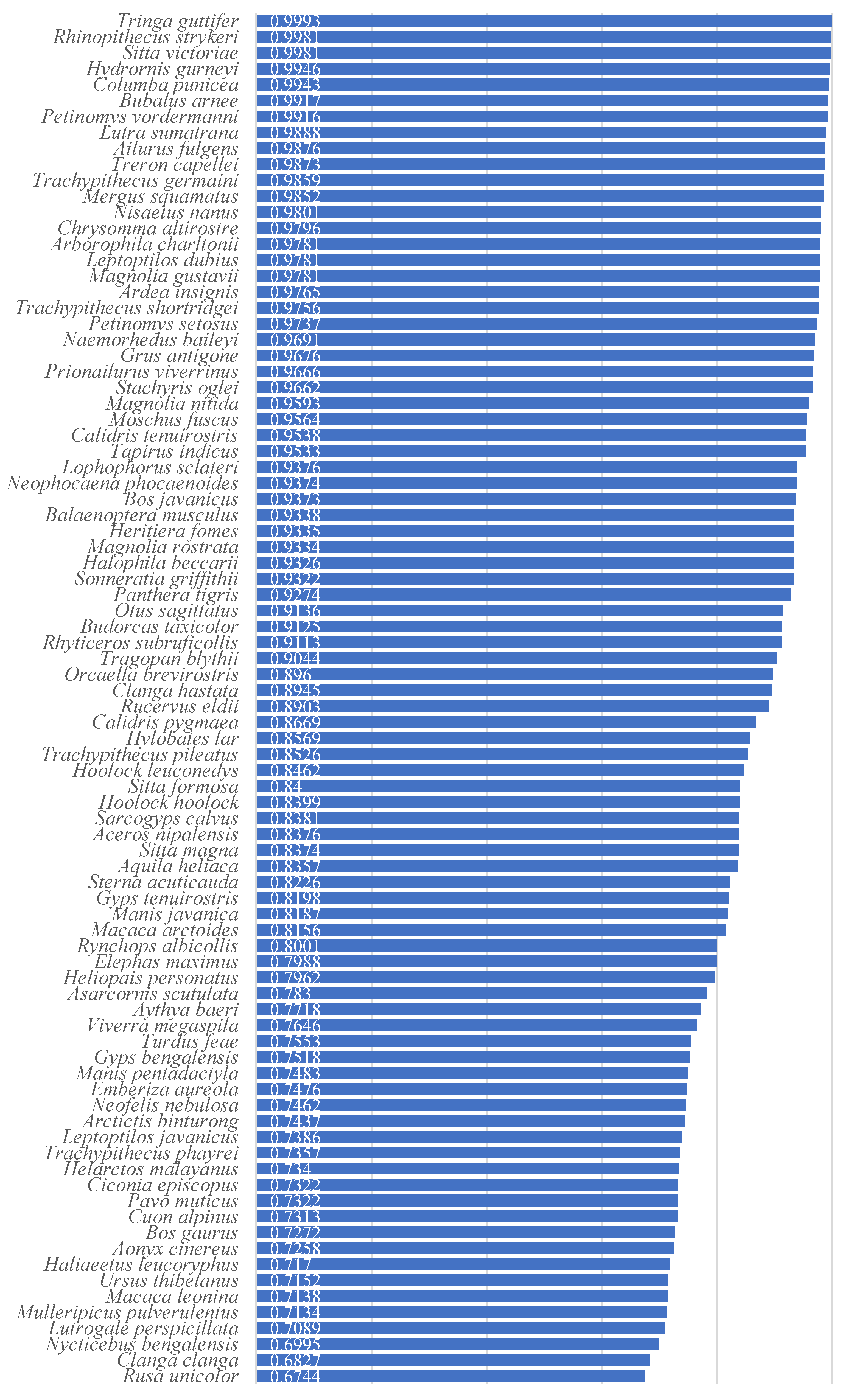
Figure 3.
ROC curve of red panda in BCC-AGCM3-MR mode under SSP126.
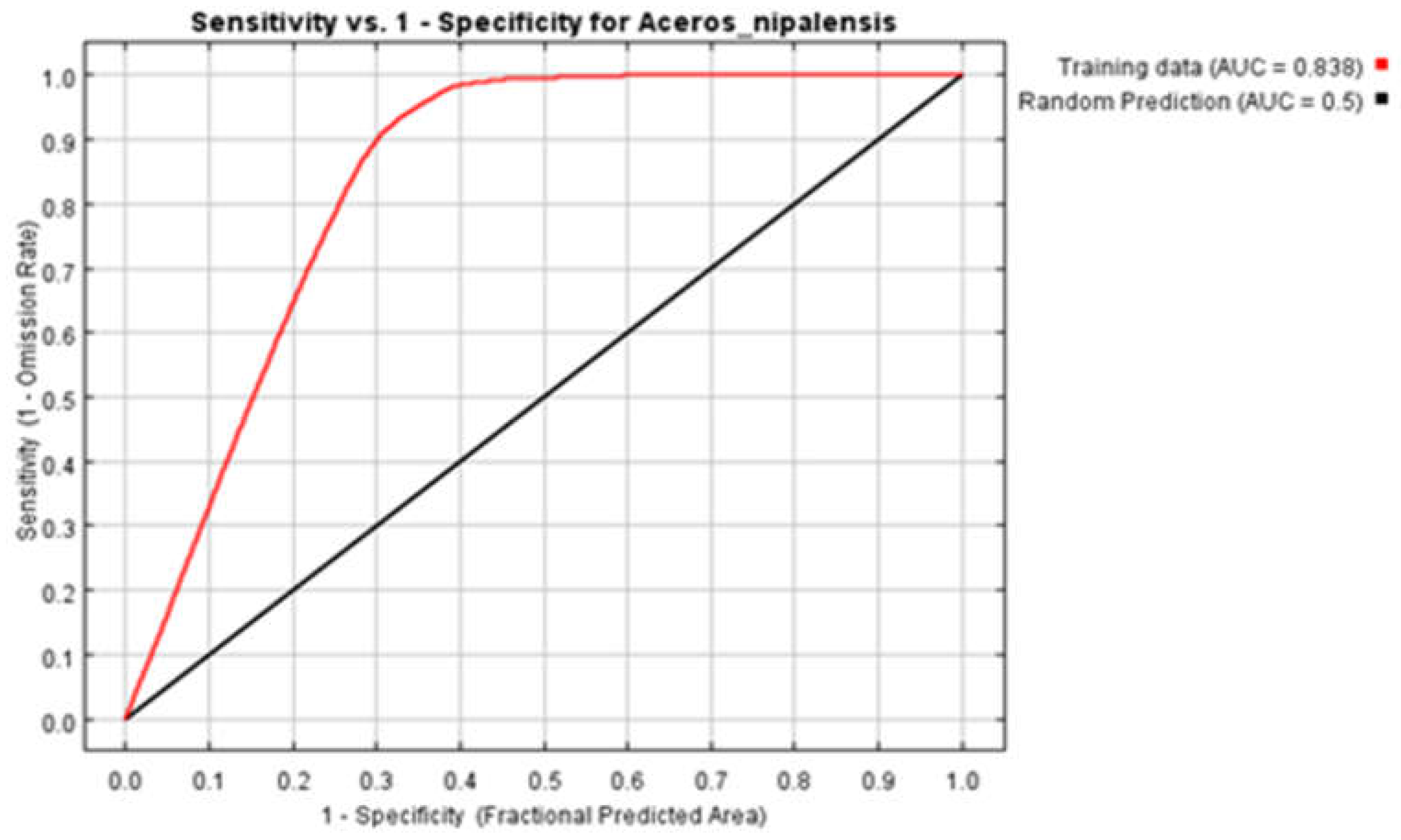
Figure 4.
Habitat changes of red pandas under different scenarios and model combinations.
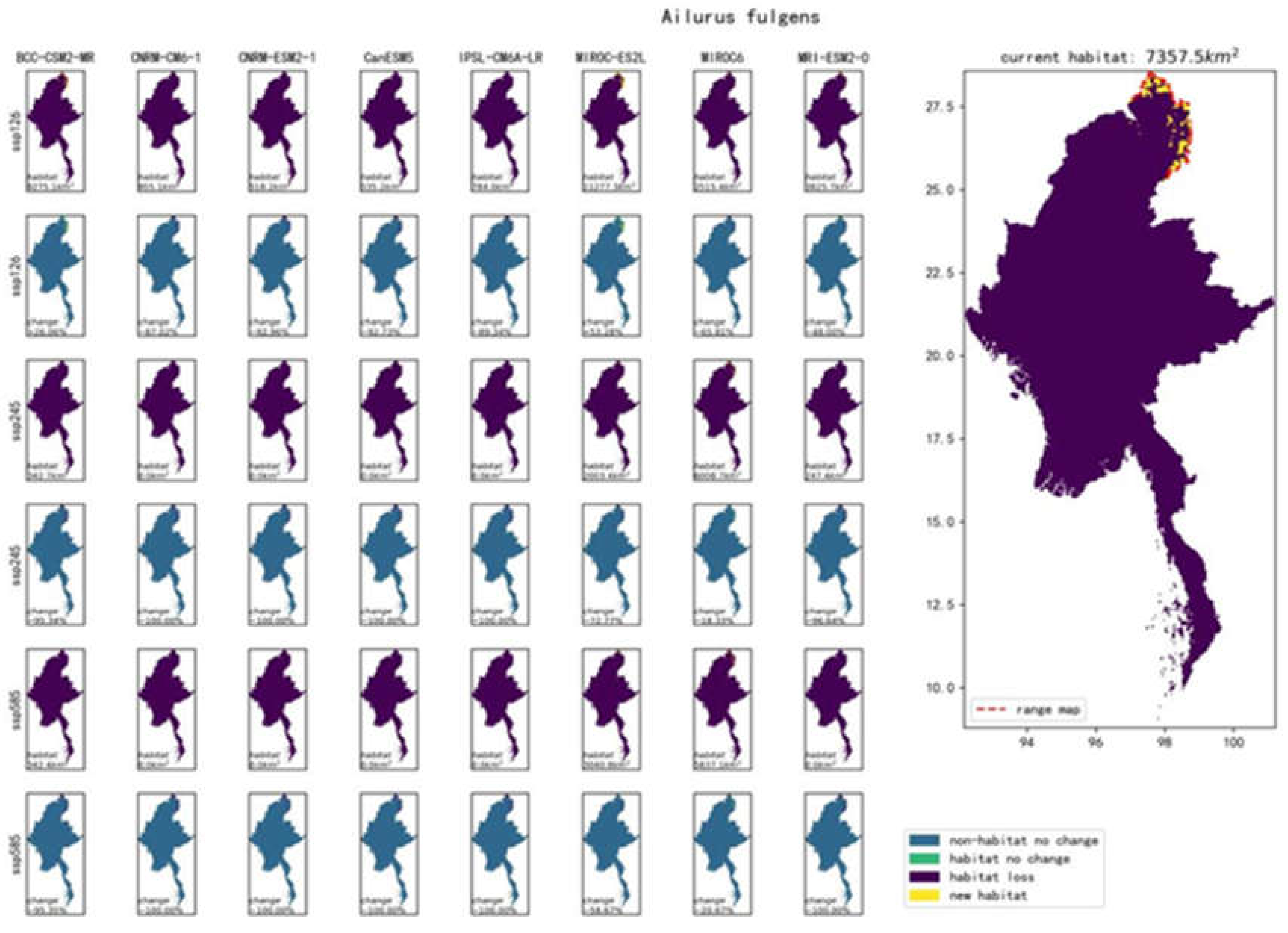
Figure 5.
Habitat assimilation of red pandas under different scenarios (binary map).
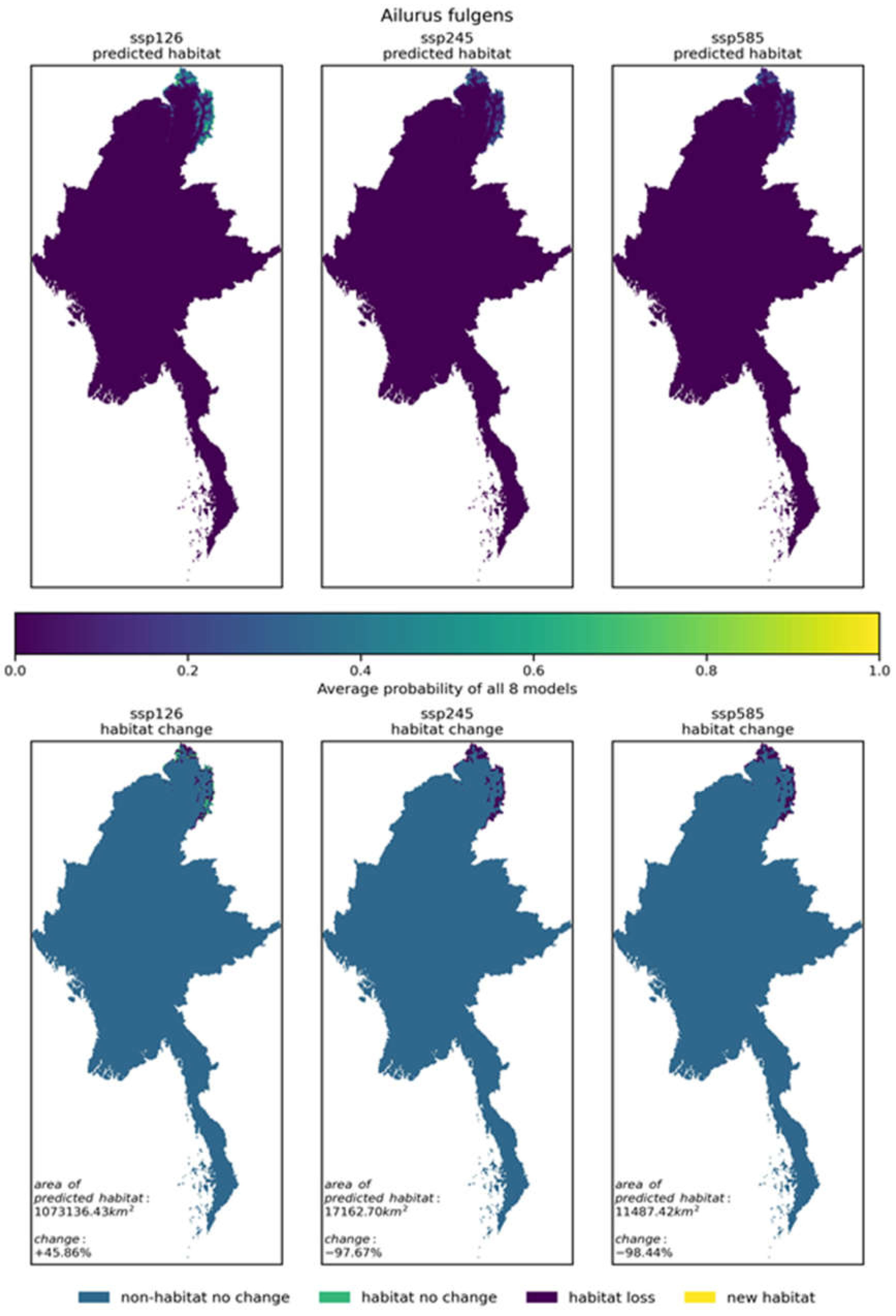
Figure 6.
Habitat assimilation of red pandas under different scenarios (probability map).
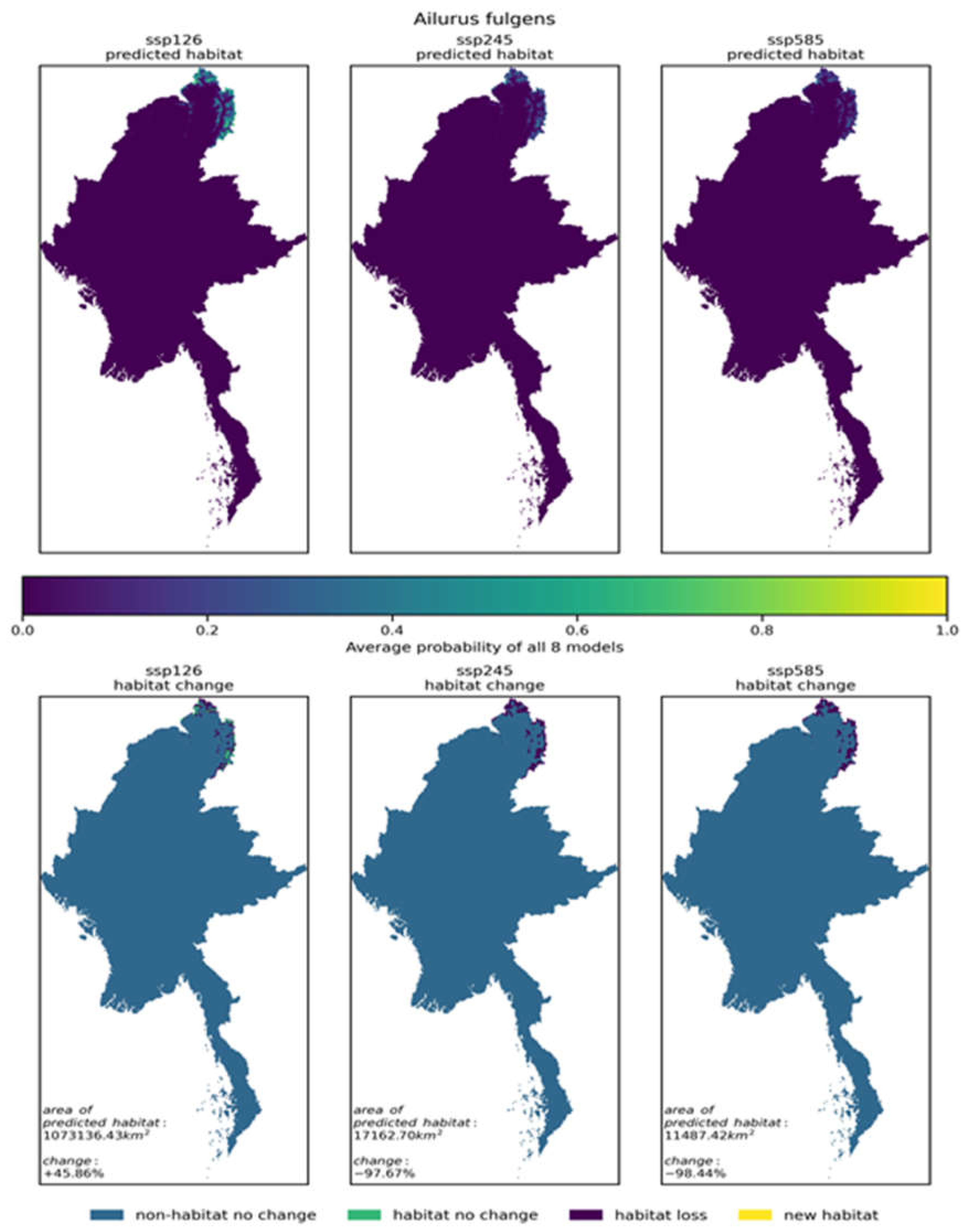
Figure 7.
The current biodiversity richness pattern of representative species in Myanmar.
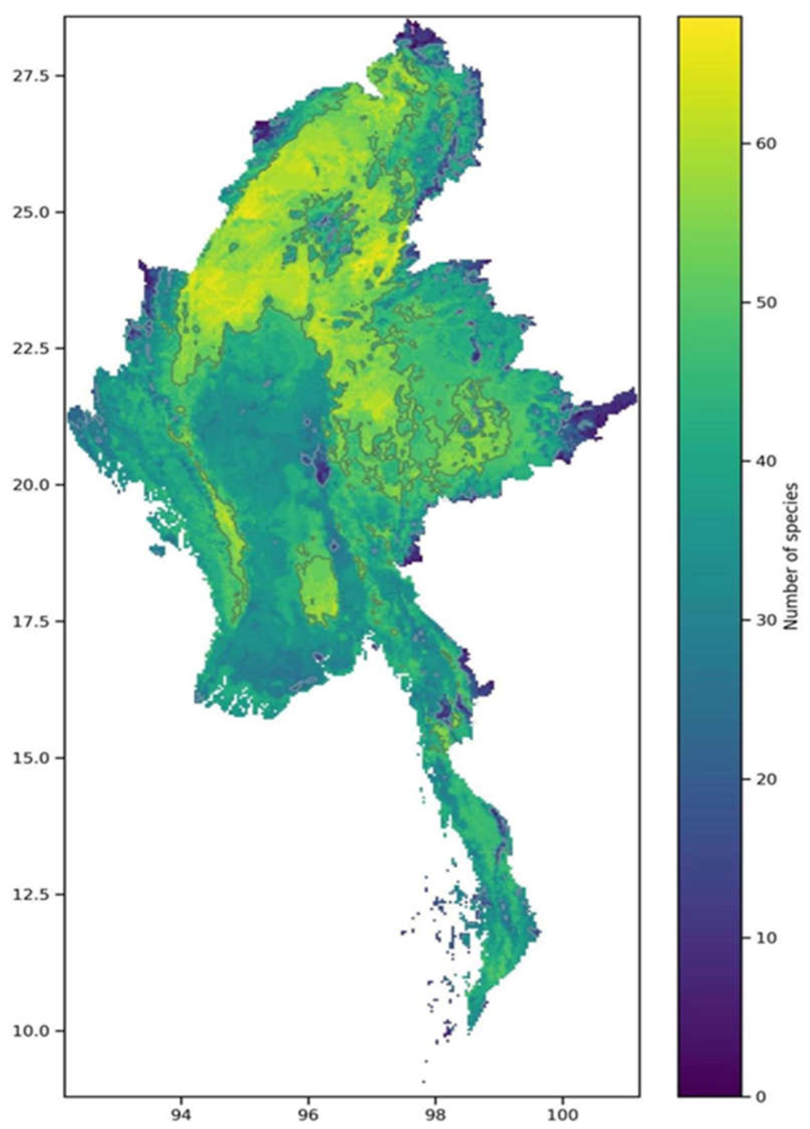
Figure 8.
Biodiversity richness pattern in Myanmar under SSP126, SSP245, and SSP585 scenarios(binary map).
Figure 8.
Biodiversity richness pattern in Myanmar under SSP126, SSP245, and SSP585 scenarios(binary map).
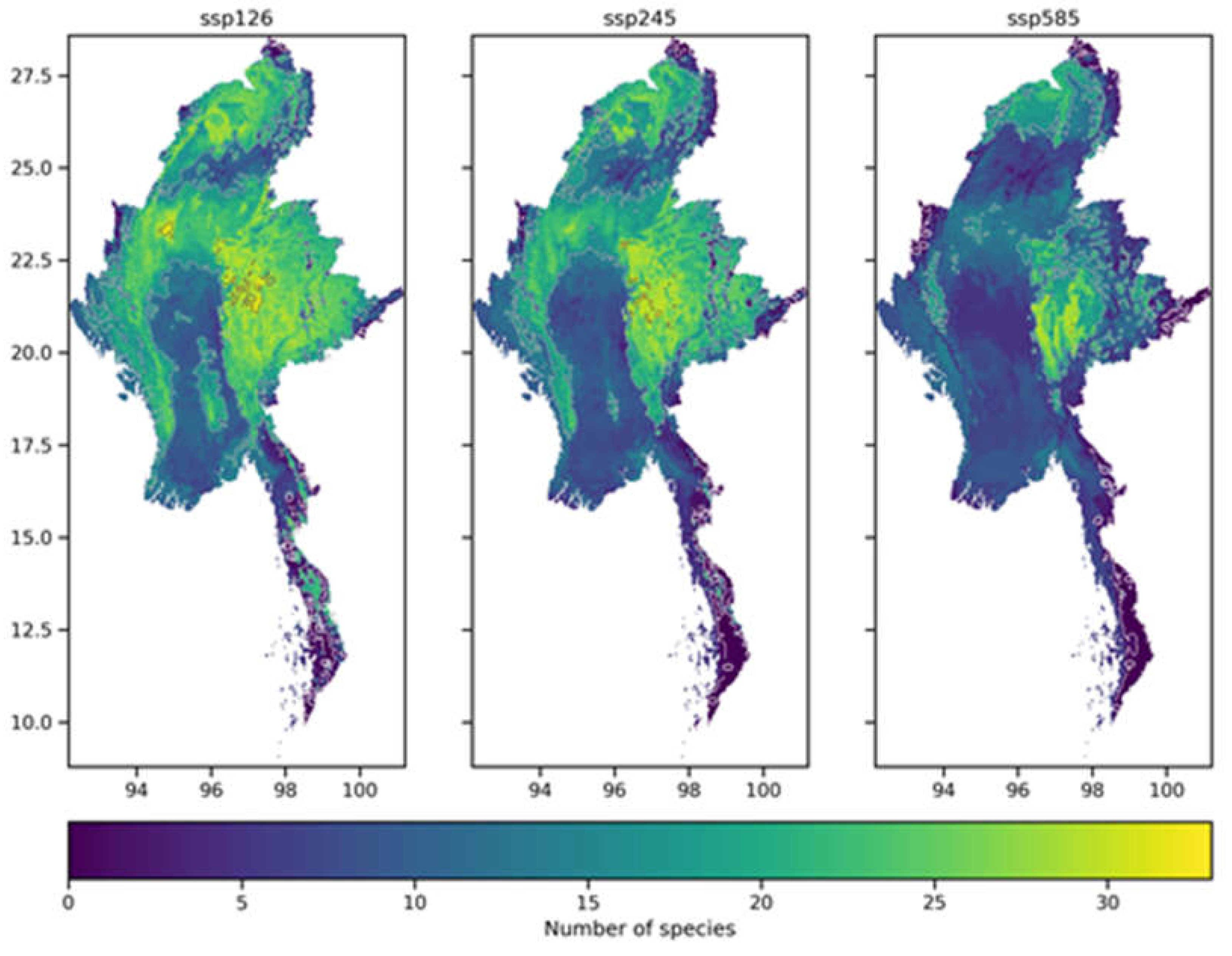
Figure 9.
Biodiversity richness pattern in Myanmar under SSP126, SSP245, and SSP585 scenarios (continuous map).
Figure 9.
Biodiversity richness pattern in Myanmar under SSP126, SSP245, and SSP585 scenarios (continuous map).

Figure 10.
Threatened situation of representative species in Myanmar under SSP126, SSP245, and SSP585.
Figure 10.
Threatened situation of representative species in Myanmar under SSP126, SSP245, and SSP585.
Figure 11.
Habitat loss status of representative species in Myanmar under SSP126, SSP245, and SSP585.
Figure 11.
Habitat loss status of representative species in Myanmar under SSP126, SSP245, and SSP585.
Figure 12.
Habitat Increase Status of Representative Species in Myanmar under SSP126, SSP245, and SSP585.
Figure 12.
Habitat Increase Status of Representative Species in Myanmar under SSP126, SSP245, and SSP585.
Figure 13.
The current pattern of biodiversity richness inside and outside protected areas in Myanmar.
Figure 13.
The current pattern of biodiversity richness inside and outside protected areas in Myanmar.
Figure 14.
Biodiversity richness patterns inside and outside Myanmar protected areas under SSP126, 245, and 585 scenarios.
Figure 14.
Biodiversity richness patterns inside and outside Myanmar protected areas under SSP126, 245, and 585 scenarios.
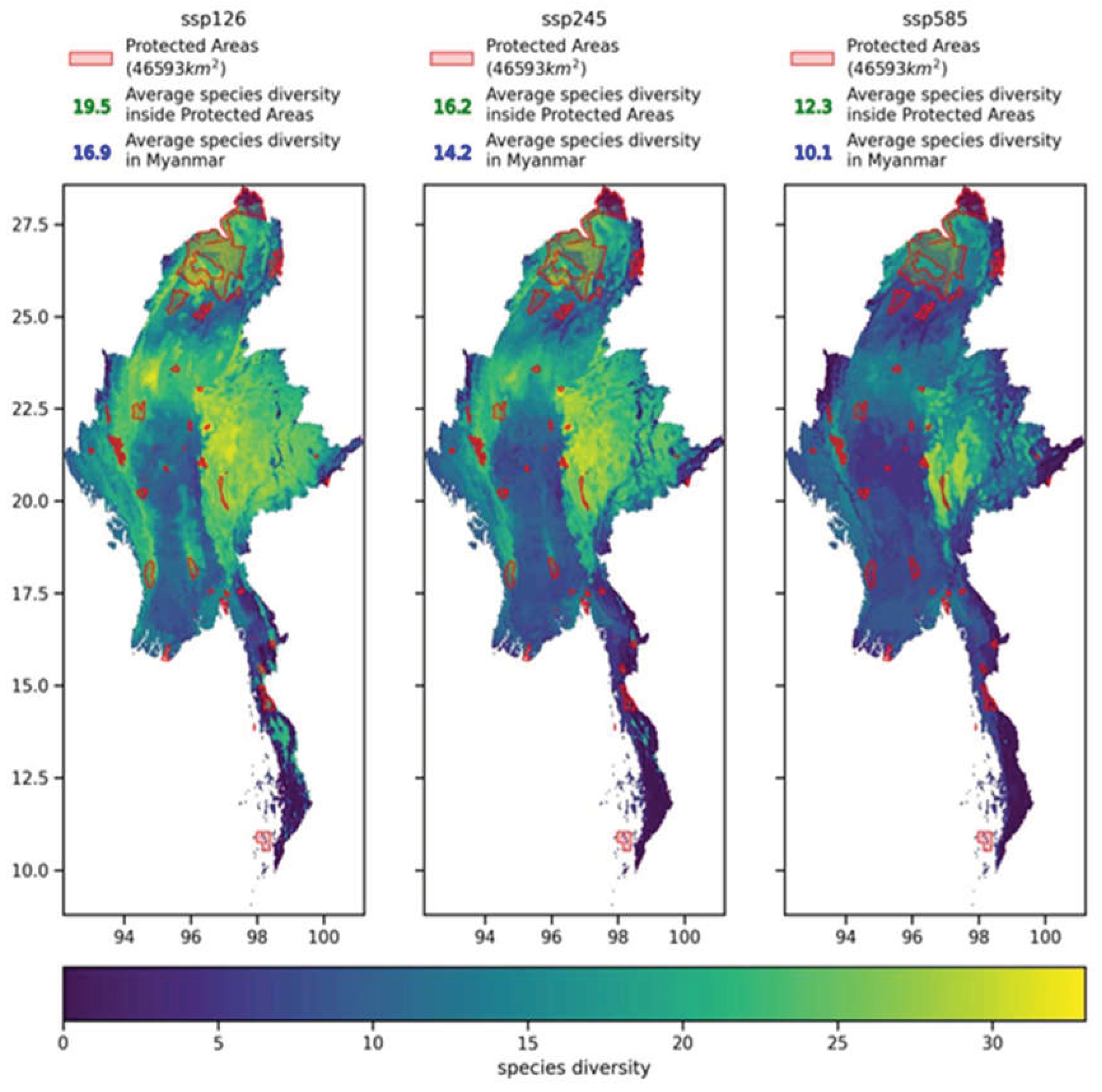
Table 1.
Overview of Myanmar Protected Areas.
| WDPA_ID |
Name |
Type |
IUCN Category |
Establishment Date |
|---|---|---|---|---|
| 1235 | Kyauk Pan Taung Wildlife Sanctuary | Wildlife Sanctuary | IV | 2013 |
| 1236 | Shwesettaw Wildlife Sanctuary | Wildlife Sanctuary | IV | 1940 |
| 1237 | Shwe-U-Daung Wildlife Sanctuary | Wildlife Sanctuary | IV | 1927 |
| 1238 | Minwuntaung Wildlife Sanctuary | Wildlife Sanctuary | IV | 1971 |
| 1239 | Kaylatha Wildlife Sanctuary | Wildlife Sanctuary | IV | 1942 |
| 8005 | Pidaung Wildlife Sanctuary | Wildlife Sanctuary | IV | 1927 |
| 8006 | Chatthin Wildlife Sanctuary | Wildlife Sanctuary | IV | 1941 |
| 8008 | Wetthikan Bird Sanctuary | Wildlife Sanctuary | IV | 1939 |
| 8009 | Taunggyi Bird Sanctuary | Wildlife Sanctuary | IV | 1920 |
| 8010 | Kahilu Wildlife Sanctuary | Wildlife Sanctuary | IV | 1928 |
| 8011 | Mulayit Wildlife Sanctuary | Wildlife Sanctuary | IV | 1935 |
| 8012 | Moscos Islands Wildlife Sanctuary | Wildlife Sanctuary | IV | 1927 |
| 8013 | Thamihla Kyun Wildlife Sanctuary | Wildlife Sanctuary | IV | 1970 |
| 8022 | Hlawga Park | Nature Park | IV | 1989 |
| 8024 | Moeyungyi Wetland Wildlife Sanctuary | Wildlife Sanctuary | IV | 1988 |
| 8027 | Natmataung National Park | Wildlife Sanctuary and ASEAN Heritage Park | II | 2010 |
| 8029 | Popa Mountain Park | Nature Park | II | 1989 |
| 8033 | Meinmahla Kyun Wildlife Sanctuary | Wildlife Sanctuary and ASEAN Heritage Park | IV | 1993 |
| 8035 | Lampi Marine National Park | Marine National Park and ASEAN Heritage Park | II | 1996 |
| 11752 | Alaungdaw Katthapa National Park | National Park and ASEAN Heritage Park | II | 1989 |
| 11813 | Inlay Lake Wildlife Sanctuary | Wildlife Sanctuary and ASEAN Heritage Park | IV | 1985 |
| 312896 | Loimwe Protected Area | Nature Reserve | IV | 1996 |
| 312897 | Parsar Protected Area | National Park | IV | 1996 |
| 312898 | Kyeikhtiyoe Wildlife Sanctuary | Wildlife Sanctuary | III | 2001 |
| 312899 | Lawkananda Sanctuary | Wildlife Sanctuary | IV | 1995 |
| 312900 | Rakhine Yoma Elephant Range | Wildlife Sanctuary | IV | 2002 |
| 312902 | Panlaung and Padalin Cave Wildlife Sanctuary | Wildlife Sanctuary | IV | 2002 |
| 312903 | Minsontaung Wildlife Sanctuary | Wildlife Sanctuary | IV | 2001 |
| 312904 | Hukaung Valley Wildlife Sanctuary (extension) | Wildlife Sanctuary | IV | 2010 |
| 312906 | Hponkanrazi Wildlife Sanctuary | Wildlife Sanctuary | IV | 2003 |
| 312910 | Bumpha Bum Wildife Sanctuary | Wildlife Sanctuary | IV | 2004 |
| 312911 | Pyin-O-Lwin Bird Sanctuary | Wildlife Sanctuary | IV | 1927 |
| 312912 | Htamanthi Wildlife Sanctuary | Wildlife Sanctuary and ASEAN Heritage Park | IV | 1974 |
| 555547903 | Taninthayi Nature Reserve | Nature Reserve | Ia | 2005 |
| 555624187 | Indawgyi Wildlife Sanctuary | Wildlife Sanctuary and ASEAN Heritage Park | IV | 2004 |
| 555624679 | Meinmahla Kyun Wildlife Sanctuary | Ramsar Site, Wetland of International Importance | Not Reported | 2017 |
| 555624853 | Gulf of Mottama | Ramsar Site, Wetland of International Importance | Not Reported | 2017 |
| 555626065 | Chungponkan Wildlife Sanctuary | Wildlife Sanctuary | IV | 2013 |
| 555626071 | Bwe Par Taung National Park | National Park | II | 2019 |
| 555626073 | Hkakaborazi National Park | National Park and ASEAN Heritage Park | II | 1998 |
| 555626074 | Hugaung Valley Wildlife Sanctuary | Wildlife Sanctuary | IV | 2004 |
| 555626075 | Inkhain Bum National Park | National Park | II | 2017 |
| 555626076 | North Zamrari Wildlife Sanctuary | Wildlife Sanctuary | IV | 2014 |
| 555626077 | Inlay Wetland W.S | UNESCO-MAB Biosphere Reserve | Not Applicable | 2015 |
| 555626078 | Indawgyi W.S | UNESCO-MAB Biosphere Reserve | Not Applicable | 2017 |
| 555626080 | Moyungyi Wetland W.S | Ramsar Site, Wetland of International Importance | Not Reported | 2004 |
| 555626095 | Indawgyi Wildlife Sanctuary | Ramsar Site, Wetland of International Importance | Not Reported | 2016 |
| 555637436 | Inlay Lake Ramsar Site | Ramsar Site, Wetland of International Importance | V | 2018 |
| 555651506 | Hpabaubg Taung Managed Nature Reserve | Nature Reserve | Not Reported | 2018 |
| 555651507 | Se Taung Wildlife Sanctuary | Wildlife Sanctuary | Not Reported | 2018 |
| 555651508 | Htaungwi Taung Geo-features Significant Area | Geo-features Significant Area | Not Reported | 2018 |
| 555703462 | Emawbum National Park | National Park | II | 2020 |
| 555703463 | Ichasaya Cave Wildlife Sanctuary | Wildlife Sanctuary | III | 2019 |
Table 2.
Contribution of climate factors to each species in the maximum entropy model.
| Species | Annual Average Temperature | Daily Range of Average Temperature | Isotherm | Seasonal Variation Coefficient of Temperature | Highest Temperature in the Hottest Month | The Lowest Temperature in the Coldest Month | Annual Temperature Range | The Average Temperature of the Wettest Quarter | Average Temperature of the Driest Quarter | The Average Temperature of the Warmest Quarter | Average Temperature of the Coldest Quarter | Annual Precipitation | Precipitation in the Wettest Month | Precipitation in the Driest month | Seasonal Variation of Precipitation | Precipitation in the Wettest Quarter | Precipitation in the Driest Quarter | Precipitation in the Warmest Quarter | Precipitation in the Coldest Quarter |
|---|---|---|---|---|---|---|---|---|---|---|---|---|---|---|---|---|---|---|---|
| Aceros nipalensis | 28.18 | 0.57 | 1.29 | 2.10 | 1.69 | 0.04 | 5.40 | 5.82 | 0.05 | 0.64 | 0.94 | 1.46 | 4.92 | 15.54 | 2.23 | 16.67 | 0.70 | 10.17 | 1.58 |
| Ailurus fulgens | 4.91 | 1.78 | 1.15 | 2.68 | 3.00 | 2.31 | 2.42 | 57.88 | 2.22 | 1.72 | 0.85 | 0.27 | 0.53 | 10.05 | 1.18 | 3.32 | 3.43 | 0.05 | 0.25 |
| Aonyx cinereus | 13.39 | 2.17 | 5.76 | 14.55 | 1.79 | 0.66 | 0.63 | 0.34 | 0.09 | 1.41 | 0.28 | 15.68 | 0.91 | 4.70 | 9.81 | 4.51 | 2.32 | 11.42 | 9.58 |
| Aquila heliaca | 30.75 | 1.25 | 3.17 | 5.14 | 0.92 | 0.00 | 7.77 | 20.92 | 0.22 | 0.05 | 0.44 | 5.30 | 4.35 | 1.69 | 0.99 | 4.55 | 5.99 | 4.48 | 2.04 |
| Arborophila charltonii | 0.01 | 2.75 | 23.24 | 36.08 | 1.27 | 0.00 | 0.24 | 0.00 | 0.04 | 0.20 | 0.07 | 2.39 | 0.00 | 5.15 | 0.01 | 0.00 | 6.79 | 0.18 | 21.57 |
| Arctictis binturong | 6.80 | 1.61 | 2.16 | 4.01 | 0.59 | 0.37 | 3.69 | 5.01 | 0.18 | 0.68 | 0.72 | 11.54 | 0.63 | 0.82 | 4.42 | 31.95 | 16.41 | 5.03 | 3.37 |
| Ardea insignis | 0.03 | 0.75 | 12.13 | 23.57 | 0.86 | 0.07 | 0.31 | 6.36 | 0.00 | 0.21 | 0.26 | 0.11 | 0.43 | 26.34 | 1.96 | 3.55 | 0.01 | 1.76 | 21.29 |
| Asarcornis scutulata | 0.55 | 2.28 | 8.35 | 8.05 | 2.01 | 0.28 | 6.02 | 6.39 | 0.09 | 0.23 | 0.05 | 7.55 | 1.81 | 0.08 | 37.18 | 12.00 | 0.37 | 1.54 | 5.18 |
| Aythya baeri | 0.35 | 4.50 | 7.92 | 31.60 | 0.88 | 4.80 | 19.99 | 4.20 | 2.44 | 0.19 | 0.51 | 1.95 | 1.07 | 1.37 | 2.14 | 0.53 | 2.14 | 1.86 | 11.53 |
| Balaenoptera musculus | 1.67 | 1.93 | 0.05 | 2.73 | 0.88 | 0.03 | 0.62 | 3.15 | 0.79 | 1.00 | 6.48 | 1.08 | 2.13 | 1.03 | 0.07 | 73.50 | 1.55 | 0.44 | 0.86 |
| Bos gaurus | 33.19 | 0.05 | 2.42 | 4.56 | 0.12 | 1.07 | 1.46 | 3.45 | 4.79 | 0.00 | 1.31 | 29.61 | 1.03 | 0.69 | 0.95 | 2.38 | 0.90 | 4.16 | 7.87 |
| Bos javanicus | 0.08 | 1.46 | 6.28 | 17.16 | 1.13 | 0.00 | 10.16 | 2.07 | 1.82 | 0.73 | 0.01 | 3.10 | 3.11 | 0.67 | 13.40 | 5.77 | 5.70 | 5.30 | 22.06 |
| Bubalus arnee | 0.00 | 0.21 | 1.62 | 4.23 | 0.19 | 0.00 | 0.20 | 0.00 | 0.00 | 0.00 | 0.00 | 0.02 | 6.80 | 13.67 | 0.00 | 3.04 | 0.61 | 69.31 | 0.09 |
| Budorcas taxicolor | 1.15 | 7.90 | 5.19 | 13.16 | 0.94 | 0.33 | 0.54 | 3.42 | 0.54 | 0.08 | 1.32 | 0.36 | 0.57 | 57.28 | 1.35 | 0.60 | 0.98 | 1.26 | 3.05 |
| Calidris pygmaea | 0.24 | 1.06 | 1.66 | 23.14 | 0.26 | 1.81 | 2.99 | 0.92 | 1.41 | 0.90 | 5.78 | 4.39 | 2.37 | 0.05 | 1.79 | 50.24 | 0.65 | 0.00 | 0.34 |
| Calidris tenuirostris | 0.64 | 0.14 | 0.02 | 3.85 | 0.08 | 0.10 | 0.32 | 0.55 | 0.04 | 0.22 | 0.00 | 0.39 | 49.87 | 0.19 | 30.59 | 1.53 | 0.75 | 10.70 | 0.01 |
| Chrysomma altirostre | 0.45 | 0.98 | 0.01 | 2.24 | 28.82 | 0.73 | 0.42 | 0.35 | 15.27 | 1.27 | 1.16 | 0.03 | 6.71 | 0.06 | 7.37 | 29.77 | 0.81 | 2.65 | 0.90 |
| Ciconia episcopus | 0.00 | 0.06 | 29.97 | 18.47 | 0.23 | 0.01 | 0.75 | 0.04 | 1.56 | 0.00 | 1.61 | 1.59 | 0.02 | 0.58 | 5.35 | 0.10 | 1.11 | 2.37 | 36.15 |
| Clanga clanga | 13.65 | 0.78 | 6.48 | 22.91 | 0.93 | 0.00 | 2.84 | 1.36 | 0.16 | 0.28 | 0.03 | 6.12 | 0.49 | 1.41 | 12.47 | 0.59 | 0.15 | 2.38 | 26.96 |
| Clanga hastata | 0.31 | 1.23 | 5.27 | 15.61 | 1.65 | 0.04 | 5.64 | 2.45 | 2.15 | 0.02 | 0.54 | 0.91 | 1.05 | 0.20 | 0.17 | 3.59 | 56.90 | 0.66 | 1.62 |
| Columba punicea | 0.00 | 0.12 | 0.14 | 10.71 | 11.14 | 0.16 | 0.23 | 0.48 | 2.18 | 0.31 | 0.13 | 0.02 | 0.59 | 0.02 | 0.99 | 46.61 | 0.09 | 21.90 | 4.18 |
| Cuon alpinus | 1.42 | 4.58 | 31.37 | 8.33 | 1.59 | 3.36 | 0.25 | 0.99 | 0.22 | 1.05 | 3.58 | 1.59 | 1.33 | 0.89 | 20.62 | 0.08 | 17.34 | 0.88 | 0.54 |
|
Elephas maximus |
16.01 | 0.64 | 7.54 | 22.93 | 0.45 | 0.08 | 0.98 | 2.63 | 2.37 | 0.01 | 0.00 | 20.06 | 2.16 | 0.17 | 10.18 | 0.01 | 9.19 | 4.00 | 0.58 |
| Emberiza aureola | 13.04 | 3.56 | 5.86 | 9.03 | 4.89 | 1.30 | 0.45 | 1.15 | 4.42 | 4.03 | 19.96 | 0.19 | 0.77 | 0.87 | 8.82 | 0.00 | 0.24 | 1.45 | 19.97 |
| Grus antigone | 0.03 | 1.46 | 8.19 | 38.61 | 0.04 | 0.47 | 9.65 | 0.12 | 0.49 | 0.03 | 0.13 | 2.91 | 0.45 | 4.86 | 1.64 | 0.27 | 7.27 | 0.55 | 22.83 |
| Gyps bengalensis | 0.00 | 0.19 | 2.65 | 27.05 | 1.08 | 0.01 | 0.44 | 1.58 | 0.08 | 1.32 | 34.11 | 16.66 | 1.34 | 0.68 | 0.48 | 0.40 | 1.21 | 1.97 | 8.75 |
| Gyps tenuirostris | 0.57 | 0.69 | 10.50 | 27.90 | 0.36 | 4.86 | 10.44 | 0.33 | 0.59 | 1.36 | 15.28 | 0.72 | 0.61 | 8.93 | 5.48 | 0.21 | 1.02 | 9.45 | 0.72 |
| Haliaeetus leucoryphus | 0.00 | 0.04 | 42.37 | 4.07 | 0.60 | 0.03 | 3.10 | 2.42 | 5.47 | 0.67 | 2.26 | 5.24 | 1.31 | 0.74 | 0.37 | 0.11 | 1.71 | 1.76 | 27.74 |
| Halophila beccarii | 0.80 | 2.71 | 0.08 | 1.41 | 0.54 | 1.89 | 1.39 | 2.32 | 3.64 | 0.08 | 8.55 | 1.41 | 0.00 | 0.01 | 1.90 | 71.27 | 0.29 | 0.22 | 1.48 |
| Helarctos malayanus | 8.10 | 6.37 | 2.95 | 2.74 | 0.55 | 0.00 | 0.75 | 6.42 | 0.32 | 19.67 | 0.27 | 28.41 | 0.33 | 0.92 | 0.59 | 13.26 | 1.07 | 3.53 | 3.75 |
| Heliopais personatus | 0.65 | 0.87 | 13.04 | 9.46 | 2.44 | 0.13 | 1.80 | 0.85 | 1.07 | 1.61 | 0.00 | 1.65 | 0.11 | 1.31 | 1.09 | 3.50 | 3.25 | 1.51 | 55.66 |
| Heritiera fomes | 1.23 | 1.88 | 0.04 | 0.69 | 0.08 | 1.64 | 2.18 | 2.45 | 0.08 | 1.16 | 7.95 | 1.07 | 2.34 | 1.09 | 1.61 | 72.69 | 0.20 | 0.35 | 1.29 |
| Hoolock hoolock | 0.14 | 24.33 | 11.09 | 2.97 | 0.90 | 0.79 | 0.79 | 1.78 | 0.51 | 0.00 | 9.58 | 0.38 | 1.90 | 4.14 | 36.29 | 0.00 | 2.55 | 0.84 | 1.04 |
| Hoolock leuconedys | 1.85 | 0.82 | 7.80 | 59.86 | 1.83 | 0.01 | 0.06 | 7.21 | 0.00 | 0.08 | 1.00 | 0.71 | 1.70 | 1.24 | 12.89 | 0.00 | 0.00 | 1.73 | 1.22 |
| Hydrornis gurneyi | 2.59 | 0.22 | 18.78 | 44.27 | 0.11 | 0.19 | 0.93 | 0.29 | 6.70 | 0.00 | 0.16 | 0.01 | 0.05 | 7.72 | 4.84 | 0.95 | 11.37 | 0.00 | 0.82 |
| Hylobates lar | 0.00 | 0.99 | 38.52 | 14.09 | 1.12 | 0.00 | 0.17 | 19.11 | 0.02 | 2.18 | 0.40 | 1.31 | 0.18 | 2.69 | 0.59 | 6.76 | 4.23 | 6.71 | 0.92 |
| Leptoptilos dubius | 0.00 | 12.73 | 7.10 | 40.32 | 0.79 | 0.00 | 0.30 | 6.65 | 4.51 | 0.00 | 0.00 | 0.31 | 2.73 | 0.00 | 1.19 | 19.57 | 1.71 | 2.08 | 0.01 |
| Leptoptilos javanicus | 0.12 | 0.56 | 23.21 | 17.27 | 0.36 | 0.53 | 0.31 | 0.73 | 0.63 | 0.01 | 0.00 | 1.49 | 0.47 | 0.98 | 9.74 | 0.33 | 0.05 | 1.23 | 41.99 |
| Lophophorus sclateri | 20.53 | 11.21 | 0.99 | 1.20 | 1.00 | 0.62 | 0.00 | 3.06 | 1.00 | 0.24 | 6.66 | 0.38 | 0.07 | 41.75 | 2.74 | 0.10 | 0.66 | 0.97 | 6.81 |
| Lutra sumatrana | 2.06 | 3.85 | 1.38 | 2.91 | 1.07 | 0.19 | 2.01 | 8.14 | 0.07 | 0.30 | 0.18 | 3.68 | 0.27 | 18.48 | 0.13 | 2.11 | 1.66 | 31.19 | 20.34 |
| Lutrogale perspicillata | 9.82 | 0.82 | 2.12 | 38.93 | 0.14 | 0.11 | 2.38 | 0.15 | 0.11 | 0.04 | 0.32 | 2.09 | 0.35 | 2.94 | 2.64 | 1.88 | 0.19 | 3.29 | 31.69 |
| Macaca arctoides | 1.40 | 6.64 | 2.30 | 6.57 | 0.89 | 0.00 | 0.06 | 6.76 | 0.00 | 0.00 | 3.78 | 5.66 | 1.08 | 2.57 | 6.81 | 33.13 | 6.91 | 2.71 | 12.74 |
| Macaca leonina | 24.93 | 0.07 | 4.70 | 15.86 | 1.73 | 0.00 | 1.43 | 4.43 | 0.42 | 0.14 | 0.98 | 24.99 | 0.38 | 0.41 | 5.21 | 2.50 | 0.19 | 2.32 | 9.32 |
| Magnolia gustavii | 9.40 | 0.65 | 31.96 | 29.50 | 0.05 | 0.05 | 1.95 | 6.56 | 4.89 | 0.01 | 0.00 | 1.07 | 2.32 | 0.08 | 0.34 | 3.61 | 5.66 | 0.27 | 1.64 |
| Magnolia nitida | 6.10 | 0.04 | 18.57 | 9.81 | 1.31 | 0.41 | 0.08 | 3.03 | 0.23 | 2.26 | 6.16 | 7.08 | 0.21 | 18.68 | 10.01 | 0.51 | 3.53 | 2.83 | 9.14 |
| Magnolia rostrata | 17.50 | 4.63 | 15.32 | 3.68 | 1.35 | 0.61 | 0.48 | 2.78 | 1.27 | 1.24 | 1.23 | 0.03 | 0.24 | 38.69 | 0.94 | 0.31 | 2.50 | 1.61 | 5.60 |
| Manis javanica | 6.65 | 1.14 | 1.86 | 53.79 | 1.51 | 0.17 | 1.86 | 6.03 | 11.10 | 0.06 | 0.09 | 0.15 | 1.24 | 1.06 | 0.26 | 0.95 | 2.83 | 8.02 | 1.23 |
| Manis pentadactyla | 0.00 | 0.10 | 1.99 | 10.03 | 0.97 | 0.05 | 1.10 | 1.10 | 0.31 | 0.06 | 49.67 | 18.25 | 0.51 | 0.65 | 1.67 | 0.11 | 2.52 | 1.83 | 9.08 |
| Mergus squamatus | 0.46 | 11.26 | 2.84 | 4.93 | 0.37 | 0.02 | 1.55 | 15.28 | 0.64 | 0.00 | 0.00 | 9.46 | 0.02 | 0.63 | 8.02 | 1.64 | 4.11 | 38.08 | 0.67 |
| Moschus fuscus | 36.81 | 2.89 | 11.96 | 4.73 | 0.04 | 0.32 | 0.91 | 2.33 | 2.15 | 1.54 | 3.93 | 0.02 | 0.01 | 16.82 | 1.42 | 0.90 | 3.77 | 0.74 | 8.70 |
| Mulleripicus pulverulentus | 11.19 | 1.59 | 5.05 | 31.97 | 0.97 | 0.67 | 1.40 | 0.14 | 2.18 | 0.82 | 3.35 | 2.59 | 0.76 | 1.90 | 17.09 | 0.31 | 0.66 | 4.00 | 13.35 |
| Naemorhedus baileyi | 29.66 | 1.06 | 38.47 | 0.97 | 1.50 | 1.63 | 0.10 | 2.25 | 3.16 | 2.43 | 0.18 | 0.00 | 0.02 | 13.22 | 1.95 | 0.99 | 0.01 | 0.36 | 2.03 |
| Neofelis nebulosa | 29.69 | 0.71 | 8.66 | 8.57 | 1.24 | 0.00 | 2.23 | 1.60 | 0.40 | 0.16 | 2.94 | 13.69 | 1.60 | 2.75 | 1.67 | 11.27 | 1.77 | 4.30 | 6.76 |
| Neophocaena phocaenoides | 2.81 | 2.19 | 0.02 | 2.76 | 0.01 | 3.03 | 1.95 | 2.08 | 2.36 | 1.04 | 0.50 | 2.52 | 4.19 | 0.89 | 0.03 | 70.17 | 1.73 | 0.37 | 1.34 |
| Nisaetus nanus | 0.13 | 3.15 | 18.32 | 26.37 | 0.01 | 0.09 | 0.85 | 0.05 | 0.00 | 0.03 | 0.01 | 5.22 | 0.16 | 0.36 | 0.00 | 0.02 | 5.13 | 0.06 | 40.04 |
| Nycticebus bengalensis | 12.39 | 0.87 | 5.52 | 10.12 | 1.06 | 0.00 | 2.22 | 3.03 | 0.29 | 0.00 | 0.04 | 33.26 | 1.10 | 0.79 | 6.84 | 2.54 | 0.22 | 4.18 | 15.52 |
| Orcaella brevirostris | 7.30 | 0.45 | 1.89 | 4.04 | 0.34 | 0.02 | 0.50 | 48.81 | 0.92 | 1.74 | 0.73 | 4.64 | 1.67 | 0.86 | 6.96 | 0.49 | 3.01 | 7.68 | 7.94 |
| Otus sagittatus | 0.00 | 2.22 | 9.48 | 63.54 | 1.52 | 0.51 | 0.07 | 6.14 | 2.49 | 0.11 | 0.09 | 0.33 | 0.20 | 0.44 | 0.33 | 9.85 | 1.31 | 1.15 | 0.22 |
| Panthera tigris | 0.00 | 2.73 | 3.17 | 5.82 | 0.63 | 0.00 | 6.84 | 4.58 | 3.88 | 0.07 | 0.00 | 6.56 | 0.76 | 8.21 | 0.85 | 1.41 | 2.58 | 38.47 | 13.45 |
| Pavo muticus | 5.25 | 9.71 | 7.16 | 24.23 | 0.01 | 0.08 | 0.55 | 0.24 | 0.47 | 0.39 | 1.11 | 1.59 | 0.13 | 1.31 | 0.53 | 2.53 | 2.62 | 0.38 | 41.70 |
| Petinomys setosus | 12.67 | 2.26 | 6.42 | 2.28 | 1.32 | 0.09 | 0.01 | 2.11 | 0.14 | 0.01 | 0.01 | 1.00 | 2.11 | 1.83 | 1.11 | 3.80 | 3.36 | 58.81 | 0.69 |
| Petinomys vordermanni | 3.61 | 3.10 | 20.10 | 46.87 | 1.24 | 0.17 | 0.86 | 0.06 | 0.09 | 0.00 | 0.08 | 6.51 | 0.00 | 9.60 | 3.37 | 0.28 | 2.95 | 1.10 | 0.00 |
| Prionailurus viverrinus | 0.29 | 1.56 | 2.02 | 20.40 | 3.38 | 0.35 | 0.00 | 0.00 | 0.22 | 0.10 | 0.30 | 0.00 | 5.07 | 0.18 | 0.37 | 45.31 | 12.77 | 7.55 | 0.13 |
| Rhinopithecus strykeri | 10.81 | 2.05 | 12.00 | 0.19 | 0.00 | 0.18 | 0.00 | 17.44 | 2.82 | 0.00 | 7.13 | 0.00 | 0.02 | 3.33 | 2.80 | 2.45 | 4.31 | 0.00 | 34.46 |
| Rhyticeros subruficollis | 2.80 | 1.47 | 2.20 | 63.32 | 1.50 | 0.01 | 0.13 | 7.07 | 2.74 | 0.12 | 0.24 | 4.55 | 0.84 | 1.32 | 3.41 | 4.71 | 2.13 | 0.89 | 0.54 |
| Rucervus eldii | 0.04 | 2.33 | 2.92 | 11.96 | 0.78 | 2.23 | 1.19 | 0.67 | 1.11 | 3.57 | 0.22 | 0.00 | 2.07 | 1.82 | 6.39 | 1.01 | 16.45 | 0.96 | 44.30 |
| Rusa unicolor | 12.99 | 1.06 | 6.87 | 14.33 | 1.00 | 0.00 | 2.51 | 2.50 | 0.28 | 1.33 | 1.49 | 7.18 | 1.65 | 1.53 | 18.06 | 0.72 | 0.40 | 1.81 | 24.29 |
| Rynchops albicollis | 1.44 | 8.78 | 5.55 | 10.10 | 1.46 | 0.00 | 2.50 | 1.01 | 1.00 | 0.58 | 0.51 | 3.03 | 0.06 | 1.75 | 1.28 | 0.13 | 1.41 | 4.30 | 55.10 |
| Sarcogyps calvus | 0.00 | 10.08 | 3.69 | 3.69 | 0.03 | 0.07 | 0.69 | 3.01 | 0.41 | 0.04 | 41.17 | 7.64 | 3.76 | 0.14 | 1.95 | 12.91 | 6.98 | 2.58 | 1.16 |
| Sitta formosa | 36.89 | 1.30 | 1.48 | 8.04 | 0.55 | 0.00 | 3.44 | 12.84 | 0.16 | 0.01 | 0.65 | 7.98 | 8.28 | 5.68 | 1.21 | 0.41 | 3.68 | 5.77 | 1.62 |
| Sitta magna | 18.21 | 21.66 | 0.98 | 18.11 | 1.05 | 0.00 | 0.04 | 20.38 | 0.62 | 0.00 | 0.16 | 6.77 | 0.04 | 2.46 | 0.58 | 5.22 | 1.25 | 2.40 | 0.09 |
| Sitta victoriae | 0.13 | 1.93 | 0.00 | 6.97 | 0.42 | 1.42 | 0.00 | 46.83 | 0.00 | 0.00 | 0.03 | 0.00 | 21.32 | 0.00 | 0.49 | 0.01 | 20.26 | 0.19 | 0.00 |
| Sonneratia griffithii | 1.56 | 1.91 | 0.15 | 1.66 | 0.70 | 2.40 | 1.53 | 2.68 | 0.35 | 0.05 | 6.16 | 1.30 | 1.91 | 1.12 | 1.04 | 73.86 | 0.15 | 0.58 | 0.87 |
| Stachyris oglei | 0.60 | 0.00 | 42.29 | 1.85 | 0.53 | 0.58 | 0.01 | 6.99 | 0.76 | 0.08 | 2.56 | 1.41 | 0.05 | 30.86 | 2.28 | 0.05 | 0.84 | 4.72 | 3.53 |
| Sterna acuticauda | 2.71 | 0.30 | 13.10 | 6.90 | 1.28 | 0.02 | 0.17 | 20.23 | 0.62 | 3.49 | 0.49 | 0.61 | 3.28 | 0.16 | 9.63 | 0.09 | 1.12 | 5.17 | 30.63 |
| Tapirus indicus | 9.61 | 1.72 | 27.67 | 47.93 | 1.28 | 0.03 | 0.18 | 1.54 | 3.10 | 0.12 | 0.01 | 2.76 | 0.22 | 0.51 | 0.26 | 1.65 | 0.94 | 0.46 | 0.04 |
| Trachypithecus germaini | 0.33 | 2.21 | 39.06 | 8.10 | 0.31 | 0.00 | 12.43 | 0.90 | 0.03 | 0.21 | 0.44 | 1.21 | 16.72 | 0.14 | 0.47 | 13.50 | 3.51 | 0.40 | 0.02 |
| Trachypithecus phayrei | 0.89 | 1.80 | 16.14 | 19.63 | 0.66 | 0.00 | 2.08 | 0.37 | 1.03 | 1.79 | 0.87 | 2.63 | 0.23 | 0.98 | 1.46 | 2.25 | 2.40 | 1.69 | 43.11 |
| Trachypithecus pileatus | 0.00 | 17.07 | 11.97 | 27.83 | 1.79 | 0.00 | 0.53 | 2.27 | 0.57 | 0.24 | 0.44 | 0.20 | 0.35 | 1.48 | 30.68 | 0.55 | 1.56 | 0.68 | 1.79 |
| Trachypithecus shortridgei | 25.91 | 1.69 | 3.36 | 4.02 | 0.90 | 0.01 | 0.00 | 2.89 | 0.05 | 0.77 | 0.44 | 0.00 | 0.00 | 18.13 | 1.52 | 0.00 | 3.36 | 0.71 | 36.25 |
| Tragopan blythii | 35.69 | 42.80 | 0.07 | 0.61 | 0.14 | 0.09 | 0.04 | 10.67 | 0.21 | 0.12 | 0.53 | 4.02 | 0.36 | 0.69 | 0.67 | 0.00 | 0.14 | 1.44 | 1.71 |
| Treron capellei | 0.14 | 0.18 | 0.90 | 57.45 | 0.01 | 1.29 | 1.41 | 0.28 | 0.95 | 0.12 | 0.09 | 1.58 | 0.00 | 0.02 | 6.44 | 13.13 | 15.59 | 0.41 | 0.00 |
| Tringa guttifer | 0.00 | 0.00 | 4.38 | 20.72 | 0.00 | 0.02 | 1.10 | 0.00 | 0.50 | 0.00 | 0.00 | 0.00 | 0.00 | 2.29 | 62.56 | 0.00 | 7.09 | 1.35 | 0.00 |
| Turdus feae | 0.00 | 0.01 | 2.43 | 64.68 | 0.18 | 2.18 | 0.20 | 1.15 | 0.01 | 0.54 | 0.28 | 12.12 | 0.03 | 1.01 | 3.23 | 0.08 | 1.10 | 3.23 | 7.54 |
| Ursus thibetanus | 12.97 | 1.14 | 2.56 | 5.33 | 0.60 | 0.29 | 1.09 | 1.86 | 0.09 | 3.46 | 1.63 | 45.23 | 0.27 | 0.80 | 3.44 | 12.21 | 0.47 | 1.03 | 5.51 |
| Viverra megaspila | 8.37 | 2.11 | 8.52 | 11.85 | 2.57 | 14.97 | 2.23 | 2.82 | 4.97 | 7.09 | 0.57 | 1.25 | 0.88 | 0.83 | 11.63 | 0.16 | 0.12 | 3.36 | 15.71 |
Table 4.
Proportion of species distribution area in protected areas.
| Species | Current | SSP126 | SSP245 | SSP585 |
|---|---|---|---|---|
| Lutra sumatrana | 72.75% | 67.05% (-7.84%) |
59.91% (-17.65%) |
0.22% (-99.70%) |
| Sitta victoriae | 67.87% | 93.61% (+37.92%) |
extinction (NA) |
extinction (NA) |
| Bubalus arnee | 67.33% | 54.03% (-19.76%) |
53.53% (-20.50%) |
0.00% (-100.00%) |
| Stachyris oglei | 55.17% | 64.66% (+17.20%) |
30.58% (-44.57%) |
10.45% (-81.05%) |
| Ailurus fulgens | 51.07% | 17.57% (-65.61%) |
24.19% (-52.63%) |
19.75% (-61.33%) |
| Naemorhedus baileyi | 51.07% | 31.57% (-38.17%) |
27.57% (-46.02%) |
6.72% (-86.85%) |
| Panthera tigris | 41.27% | 59.20% (+43.45%) |
56.24% (+36.29%) |
1.86% (-95.49%) |
| Rhinopithecus strykeri | 38.94% | 16.59% (-57.41%) |
2.03% (-94.80%) |
extinction (NA) |
| Petinomys setosus | 38.18% | 0.00% (-100.00%) |
0.00% (-100.00%) |
0.00% (-100.00%) |
| Moschus fuscus | 36.42% | 17.22% (-52.73%) |
7.88% (-78.36%) |
5.21% (-85.69%) |
| Magnolia rostrata | 36.05% | 29.36% (-18.55%) |
18.31% (-49.20%) |
4.94% (-86.31%) |
| Budorcas taxicolor | 33.84% | 28.57% (-15.58%) |
16.65% (-50.79%) |
3.48% (-89.73%) |
| Lophophorus sclateri | 32.01% | 23.14% (-27.72%) |
13.70% (-57.21%) |
3.31% (-89.67%) |
| Ardea insignis | 25.73% | 20.62% (-19.88%) |
13.86% (-46.15%) |
6.10% (-76.28%) |
| Trachypithecus shortridgei | 23.28% | 4.88% (-79.05%) |
0.75% (-96.76%) |
0.88% (-96.23%) |
| Aceros nipalensis | 21.31% | 15.19% (-28.72%) |
13.54% (-36.46%) |
18.15% (-14.80%) |
| Tragopan blythii | 21.31% | 19.67% (-7.66%) |
19.54% (-8.30%) |
27.40% (+28.60%) |
| Magnolia nitida | 20.30% | 8.91% (-56.12%) |
7.58% (-62.67%) |
6.39% (-68.53%) |
| Trachypithecus pileatus | 20.20% | 16.84% (-16.64%) |
15.26% (-24.43%) |
15.85% (-21.51%) |
| Macaca arctoides | 19.68% | 18.80% (-4.46%) |
10.09% (-48.72%) |
8.45% (-57.09%) |
| Hoolock leuconedys | 17.93% | 15.64% (-12.77%) |
11.83% (-34.02%) |
10.93% (-39.05%) |
| Hoolock hoolock | 16.61% | 14.42% (-13.15%) |
12.66% (-23.77%) |
14.41% (-13.23%) |
| Sitta formosa | 15.23% | 11.14% (-26.85%) |
10.13% (-33.49%) |
12.14% (-20.27%) |
| Aquila heliaca | 10.82% | 8.92% (-17.61%) |
11.34% (+4.80%) |
16.85% (+55.71%) |
| Asarcornis scutulata | 10.78% | 9.49% (-12.01%) |
8.53% (-20.92%) |
7.74% (-28.25%) |
| Neofelis nebulosa | 10.70% | 12.16% (+13.58%) |
11.74% (+9.72%) |
17.54% (+63.83%) |
| Helarctos malayanus | 9.86% | 7.95% (-19.31%) |
8.98% (-8.95%) |
12.60% (+27.85%) |
| Turdus feae | 9.62% | 8.48% (-11.87%) |
7.41% (-23.00%) |
13.36% (+38.82%) |
| Elephas maximus | 9.55% | 11.09% (+16.08%) |
11.24% (+17.64%) |
16.52% (+72.96%) |
| Gyps bengalensis | 9.54% | 8.92% (-6.49%) |
7.92% (-16.94%) |
16.00% (+67.76%) |
| Manis pentadactyla | 9.44% | 9.89% (+4.77%) |
9.28% (-1.65%) |
16.69% (+76.87%) |
| Cuon alpinus | 9.41% | 9.19% (-2.39%) |
9.05% (-3.84%) |
10.98% (+16.59%) |
| Bos gaurus | 8.82% | 8.69% (-1.50%) |
7.63% (-13.54%) |
13.12% (+48.78%) |
| Arctictis binturong | 8.65% | 7.54% (-12.85%) |
7.14% (-17.43%) |
8.85% (+2.32%) |
| Aonyx cinereus | 8.51% | 7.43% (-12.69%) |
6.81% (-19.91%) |
8.13% (-4.47%) |
| Ursus thibetanus | 8.35% | 8.13% (-2.72%) |
7.79% (-6.79%) |
11.78% (+40.96%) |
| Macaca leonina | 7.50% | 7.86% (+4.71%) |
6.74% (-10.14%) |
10.24% (+36.39%) |
| Nycticebus bengalensis | 7.16% | 8.20% (+14.58%) |
9.56% (+33.48%) |
12.92% (+80.53%) |
| Viverra megaspila | 7.04% | 10.94% (+55.34%) |
12.83% (+82.17%) |
18.47% (+162.14%) |
| Haliaeetus leucoryphus | 6.79% | 6.66% (-2.04%) |
6.10% (-10.24%) |
6.34% (-6.68%) |
| Tapirus indicus | 6.55% | 9.36% (+42.89%) |
5.16% (-21.16%) |
0.00% (-100.00%) |
| Rusa unicolor | 6.45% | 7.59% (+17.57%) |
7.79% (+20.70%) |
10.94% (+69.45%) |
| Magnolia gustavii | 6.23% | 3.13% (-49.73%) |
2.43% (-61.06%) |
0.00% (-100.00%) |
| Clanga clanga | 6.10% | 7.45% (+22.12%) |
8.75% (+43.31%) |
12.81% (+109.89%) |
| Mulleripicus pulverulentus | 5.61% | 6.77% (+20.74%) |
7.08% (+26.29%) |
10.34% (+84.40%) |
| Sterna acuticauda | 5.13% | 5.66% (+10.33%) |
5.39% (+4.99%) |
3.44% (-32.95%) |
| Bos javanicus | 4.95% | 8.59% (+73.54%) |
7.59% (+53.37%) |
4.89% (-1.15%) |
| Leptoptilos dubius | 4.74% | 2.78% (-41.25%) |
2.07% (-56.26%) |
1.84% (-61.17%) |
| Rhyticeros subruficollis | 4.60% | 3.37% (-26.74%) |
2.10% (-54.40%) |
1.46% (-68.24%) |
| Columba punicea | 4.51% | 0.00% (-100.00%) |
extinction (NA) |
extinction (NA) |
| Otus sagittatus | 4.48% | 7.08% (+58.02%) |
3.67% (-18.02%) |
0.97% (-78.36%) |
| Emberiza aureola | 4.36% | 6.68% (+53.35%) |
7.62% (+74.83%) |
6.88% (+57.94%) |
| Gyps tenuirostris | 4.23% | 1.37% (-67.51%) |
3.09% (-26.89%) |
5.58% (+31.89%) |
| Leptoptilos javanicus | 4.15% | 3.83% (-7.62%) |
3.76% (-9.40%) |
4.23% (+1.92%) |
| Trachypithecus germaini | 4.12% | 1.93% (-53.22%) |
0.00% (-100.00%) |
0.00% (-100.00%) |
| Calidris pygmaea | 3.98% | 5.98% (+50.04%) |
11.98% (+200.70%) |
25.39% (+537.29%) |
| Ciconia episcopus | 3.71% | 4.39% (+18.48%) |
3.62% (-2.28%) |
3.62% (-2.36%) |
| Neophocaena phocaenoides | 3.32% | 2.77% (-16.61%) |
2.43% (-26.70%) |
2.00% (-39.87%) |
| Manis javanica | 3.31% | 2.66% (-19.52%) |
2.66% (-19.74%) |
0.64% (-80.62%) |
| Heritiera fomes | 3.23% | 2.28% (-29.55%) |
2.66% (-17.64%) |
6.87% (+112.23%) |
| Sonneratia griffithii | 3.16% | 2.36% (-25.48%) |
2.50% (-21.05%) |
2.68% (-15.36%) |
| Clanga hastata | 3.12% | 2.87% (-7.82%) |
13.60% (+336.53%) |
0.00% (-100.00%) |
| Balaenoptera musculus | 3.11% | 2.27% (-27.11%) |
2.63% (-15.33%) |
2.69% (-13.64%) |
| Halophila beccarii | 3.09% | 2.32% (-24.84%) |
2.65% (-14.13%) |
2.64% (-14.37%) |
| Rucervus eldii | 2.78% | 2.77% (-0.44%) |
2.44% (-12.06%) |
2.25% (-18.87%) |
| Aythya baeri | 2.73% | 1.91% (-29.96%) |
1.48% (-45.84%) |
1.13% (-58.48%) |
| Orcaella brevirostris | 2.39% | 4.22% (+76.72%) |
5.64% (+136.02%) |
8.16% (+241.78%) |
| Lutrogale perspicillata | 2.26% | 2.67% (+18.37%) |
2.84% (+25.97%) |
2.50% (+10.75%) |
| Hylobates lar | 2.25% | 1.96% (-13.01%) |
1.29% (-42.88%) |
0.62% (-72.64%) |
| Heliopais personatus | 2.09% | 2.30% (+10.04%) |
2.25% (+7.97%) |
2.46% (+18.10%) |
| Prionailurus viverrinus | 2.05% | 3.88% (+89.20%) |
6.36% (+210.07%) |
4.15% (+102.12%) |
| Pavo muticus | 2.00% | 1.68% (-16.12%) |
1.41% (-29.71%) |
0.95% (-52.61%) |
| Sarcogyps calvus | 1.87% | 0.60% (-67.69%) |
0.14% (-92.31%) |
1.20% (-35.82%) |
| Grus antigone | 1.79% | 0.88% (-50.89%) |
0.00% (-100.00%) |
extinction (NA) |
| Rynchops albicollis | 1.74% | 1.78% (+2.12%) |
1.78% (+1.99%) |
1.46% (-15.91%) |
| Trachypithecus phayrei | 1.63% | 1.71% (+4.71%) |
1.72% (+5.40%) |
1.88% (+15.31%) |
| Sitta magna | 1.01% | 1.21% (+20.01%) |
1.45% (+44.01%) |
0.16% (-84.09%) |
| Chrysomma altirostre | 0.05% | 0.03% (-39.53%) |
0.03% (-43.92%) |
0.33% (+547.42%) |
| Hydrornis gurneyi | 0.00% | 0.00% (NA) |
0.00% (NA) |
extinction (NA) |
| Calidris tenuirostris | 0.00% | 0.00% (NA) |
0.00% (NA) |
0.00% (NA) |
| Petinomys vordermanni | 0.00% | 0.00% (NA) |
0.00% (NA) |
0.00% (NA) |
| Treron capellei | 0.00% | 0.00% (NA) |
0.00% (NA) |
0.00% (NA) |
| Tringa guttifer | 0.00% | 0.00% (NA) |
extinction (NA) |
extinction (NA) |
| Mergus squamatus | 0.00% | 0.00% (NA) |
0.00% (NA) |
extinction (NA) |
| Arborophila charltonii | 0.00% | 0.00% (NA) |
0.00% (NA) |
extinction (NA) |
| Nisaetus nanus | 0.00% | 0.00% (NA) |
extinction (NA) |
extinction (NA) |
Disclaimer/Publisher’s Note: The statements, opinions and data contained in all publications are solely those of the individual author(s) and contributor(s) and not of MDPI and/or the editor(s). MDPI and/or the editor(s) disclaim responsibility for any injury to people or property resulting from any ideas, methods, instructions or products referred to in the content. |
© 2024 by the authors. Licensee MDPI, Basel, Switzerland. This article is an open access article distributed under the terms and conditions of the Creative Commons Attribution (CC BY) license (http://creativecommons.org/licenses/by/4.0/).
Copyright: This open access article is published under a Creative Commons CC BY 4.0 license, which permit the free download, distribution, and reuse, provided that the author and preprint are cited in any reuse.


