1. Introduction
There are tools developed at the beginning of the 20th century in the field of statistical quality control (SQC) widely recognised and used in the scope of industrial processes. These tools are aimed at reducing the variability of quality relating to a product or a process.
The variability of quality represents the deviation of its value with regard to the proposed objectives. The causes of variability are divided into two categories, namely: common and special. Common or random causes are inherent to the process, whereas the special or assignable causes arise due to those that are not part of the process. Since the latter are not part of the process, they can easily be removed when identified. A process is under statistical control when there is only random variability [
1]. In the last century, statistical process control (SPC)―which is part of SQC―has proven to be a successful methodology that allows monitoring the variability and stability of essential and continuous industrial processes over time [
2]. The approach of variability analysis through functional data analysis (FDA) is much more recent, and its use widespread as an analysis tool during the first years of the 21st century.
The present study consists of the development of a methodology for the analysis of variability, based on the construction of a hybrid method, i.e., functional process control (FPC), that combines the advantages of SPC and FDA. The structure of this article consists of a brief description of SPC and FDA in order to lay the theoretical and mathematical foundations of FPC, understood as a hybrid method that brings together the advantages (i.e., the capacity of detecting atypical values) of the two methods previously mentioned. After the theoretical discussion of the method, we present the results of its application in a specific case study. Finally, we present the main conclusions drawn from our work.
2. Mathematical Background
2.1. Statistical Process Control (SPC)
SPC charts were first used in 1924 by Walter Andrew Shewhart with the clear purpose of improving quality. In his study, Shewhart [
3] laid the foundations of what currently constitutes the most accepted and used tool for the detection of variability in industrial processes, monitoring them over time in order to observe changes in their performance. In addition, the goal of this method is to determine whether the process under study is stable and repeatable with respect to the variable to be controlled. This way, the ultimate aim of FPC is to improve the stability of the processes in order to improve their capacity through the reduction of variability.
Standard Shewhart’s control charts are perfect tools for the detection of assignable variability. On the one hand, their main features are sensitivity in the detection of large deviations of the μ mean of a process (three times its standard deviation [σ]), and their insensitivity in the detection of minor deviations [
4], corrected by the implementation of different sets of supplementary rules [
5]. On the other hand, there is negative influence, reflected in increased false alarms that warn about changes in the mean and effects, such as non-normality of data distribution and the phenomenon of auto-correlation in temporal series [
4,
6,
7]. It should be added that control charts detect variability, but based on a discreet approach to the problem. Shewhart’s control charts can be used to asses data in order to determine whether a process is under control or not (Phase 1 of the FPC), or samples taken sequentially to detect changes in a process under statistical control (Phase 2 of the FPC).
The goal in phase 1 is to build experimental control limits based on preliminary sampling. The aim is to determine whether the process is under control or not and, thus, use the calculated limits to control future production. The calculation process of these experimental limits consists of studying the points that are out of control looking for causes of assignable variation, so that they can be excluded from the sample and the limits recalculated. This procedure is repeated until all sample points are under control, and these limits will be used in phase 2.
Once reliable control limits have been obtained, the next phase is the operation with control charts in real time for monitoring the process. This phase is called phase 2 of the FPC, and it is the time in which the different sets of rules are used to interpret the charts through the detection of deviations and patterns. With respect to phase 2, in general terms, it is correct to assume that the process will be reasonably stable, since changes in it should be smaller, given that really large sources of assignable variations were eliminated in a systematic manner in phase 1. Therefore, Shewhart’s control charts―which are not very sensitive to small to moderate changes in the average of the process to be monitored―should be complemented with supplementary rules [8-12] due to the risk of increased number of false alarms [
2,
12,
13].
2.2. Functional Data Analysis (FDA)
High dimension and functional data are gaining importance in the field of classification due to the technological advances that allow their capture and treatment. The fundamental goal of FDA in the present study was the detection and elimination of variability [
14]. Traditionally, FDA has been applied to sets of observations of random and continuous processes monitoring discrete points [
15]. The use of functional data entails some peculiarities at the time of their treatment, mainly due to three features, namely: dimension; correlation; and the fact of working in functional spaces. The main obstacle is treating these data computationally, because the problem should be addressed resorting to the discretisation of the function, or its expression in a reduced base of the functions space (smoothing), with the consequent loss of information.
It is necessary to make some observations about the procedure to determine functional outliers. In the first place, the purpose behind this procedure is identifying the atypical functional values, such as the curves whose depths are the lowest extreme values by virtue of the distribution of the considered functional depth (FMD, HMD) [
16]. This concept is used to obtain the cut-off point (C). Secondly, the main contribution of the procedure is identifying those curves that require greater attention. This way, once that a set of atypical values is detected, it is fundamental to identify the reasons by which these paths have a different behaviour than the rest.
FDA has the following advantages in comparison to other traditional statistical methods used for the detection of outliers [
17,
18]:
Independence from the statistical data distribution, since the analysis is not performed with the original data, but with constructed functions.
Single-unit temporal analysis. The analysis of the temporal axis is set as a single unit. The sample is analysed taking into consideration the units of entire time, i.e., there are no specific values recorded in particular cases.
Analysis of trends. These techniques not only allow determining atypical values, but also the analysis of situations in which the goal is detecting small deviations.
Homogeneity analysis. The atypical values are not determined, but only those that exceed a determined limit without a possible conclusion with regard to whether it is a single or a periodic case; i.e., different points do not exceed the cut-off point, but small deviations occur constantly.
3. Functional Process Control (FPC)
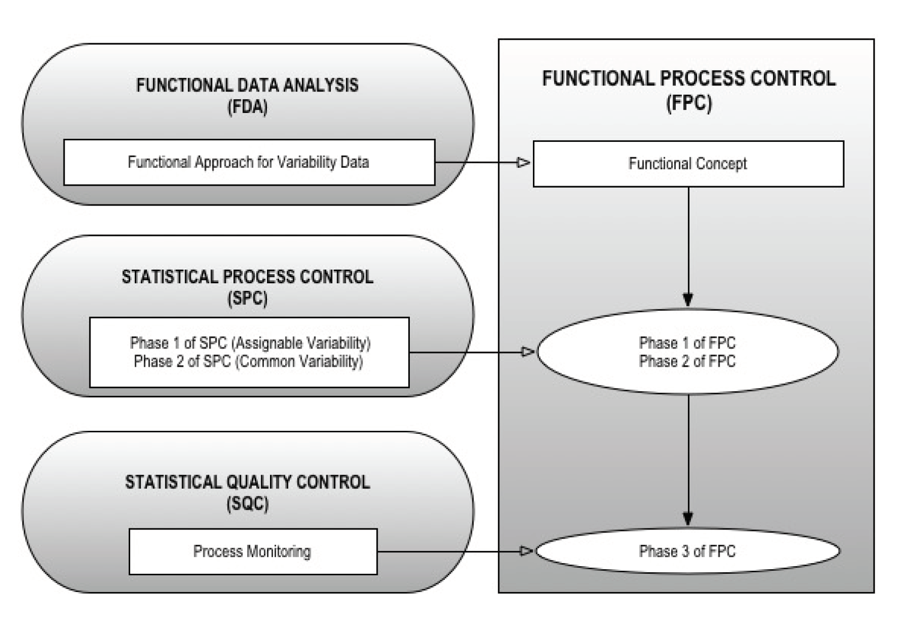
The main purpose of the present study was the implementation of a hybrid methodology called FPC, based on the FDA methodology combined with the advantages of FPC, thereby generating a toll to detect large and small functional deviations. The three phases of the FPC proposed as the backbone of the methodology are: (1) stabilisation of the process through the identification and elimination of special causes of functional variability; (2) active improvement of the process through the minimisation of the common causes of functional variability; and (3) supervision of the process to ensure the maintenance of the improvements, and the incorporation of additional improvements as different opportunities arise (
Figure 1).
3.1. Identification and Elimination of Special Causes of Functional Variability; Stabilisation of the Process (Phase 1)
Similarly to phase 1 of the SPC, the goal is to build experimental control limits based on preliminary samples. In the case of FDA, control limits correspond to the cut-off point that determines the functional outliers from the distribution of functional depths. The calculation process of this new cut-off point consists of studying the functional outliers in order to find the causes of assignable variation. If an assignable cause is identified for an outlier, it is excluded from the original functional sample and the cut-off point is again recalculated. This procedure is repeated until the original functional sample does not exhibit outliers, adopting the cut-off point as the starting point for phase 2 (
Figure 2).
3.2. Minimisation of Common Causes of Functional Variability; Active Improvement of the Process (Phase 2)
The development of phase 2 of FPC (
Figure 2) consists of: (1) determining the distribution of functional depths resulting from phase 1; (2) studying the possible adjustment of functional depths distribution calculated for a continuous probability distribution using methods based on probability charts and goodness-of-fit tests; (3) calculating the parameters and main statistical data of the continuous probability distribution corresponding to the adjustment; (4) applying the supplementary rules resulting from phase 2 of the SPC to control minor deviations; and (5) creating the standard Shewhart’s control charts with additional rules for the depths obtained after phase 1. In case goodness-of-fit measures are not obtained in step 2, Box-Cox or Johnson type transformations will be applied to normalise the distribution of depths. This way, it will be possible to obtain the empirical distribution corresponding to the distribution of depths if the previous transformation is not possible.
3.3. Assurance and Incorporation of Improvements; Supervision of the Process (Phase 3)
The processes should be monitored after they are stabilised and under statistical control, because this is an essential part of the closing phase of any continuous improvement cycle. The phase 3 of the FPC should be substantiated on the basis of the two most known and used improvement cycles, namely: the plan-do-check-act (PDCA) cycle; and the Deming, or define, measure, analyse, improve and control (DMAIC) cycle.
4. Case Study
Data in
Table 1 are simulated corresponding to 36 functional depth values (data set 1).
4.1. Phase 1 of FCP
For the data set of functional depth (Table I), the original cut-off value, after steps 1 and 2 (smoothing and bootstrapping process, respectively), was equal to 10.12 (
Figure 3).
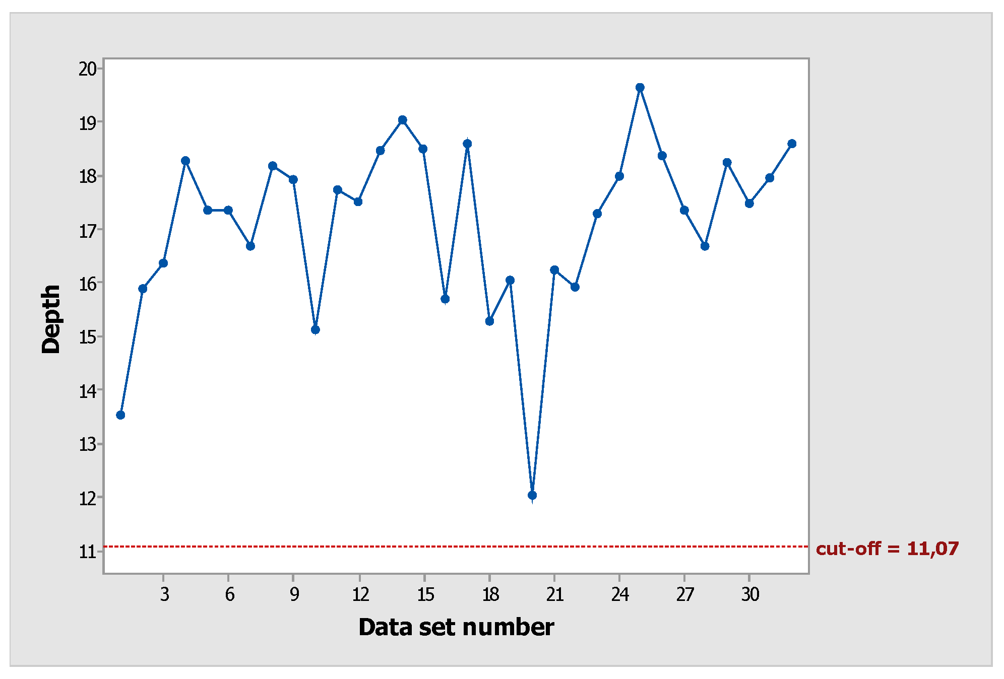
Thus, the identified functional outliers 11, 12, 13, and 14 (red points) corresponded to the functional outliers from the original functional set (step 3.1), and a new functional sample had to be calculated. As a result, the new functional depths and the new cut-off values were equal to 11.07 (
Figure 4).
At this moment, since functional outliers were not obtained, the functional depth sample (data set 2) was the starting point for phase 2 of FPC (
Figure 2).
4.2. Phase 2 of FCP
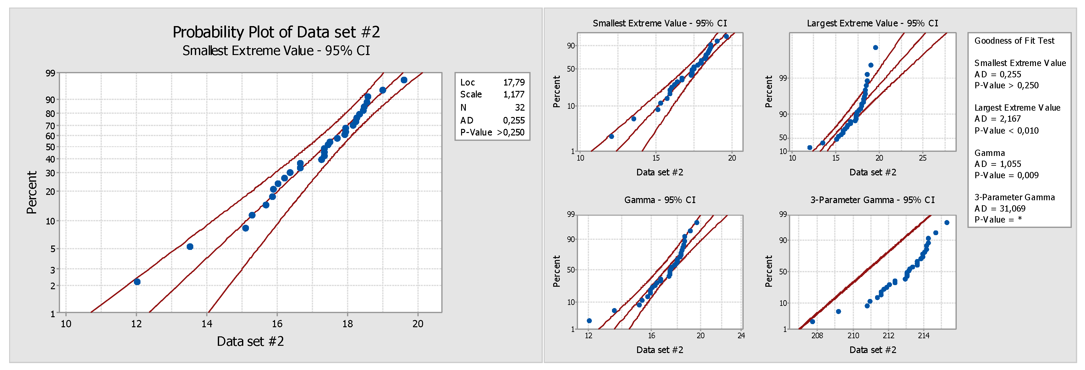
For phase 2, the functional depth sample (data set 2) obtained in phase 1 had to be fitted (step 1) by means of hypothesis testing to a known statistical probability distribution. In order to choose the best option, some probability distributions were tested (
Figure 5).
Results of the hypothesis test and the determined depth distribution could be fitted as:
Logistic distribution (p-value = 0.080), log-logistic distribution (p-value = 0.031), smallest extreme value (p-value >0.25), and Weibull distribution (p-value >0.5)
Normal after Johnson transformation (p-value = 0.767)
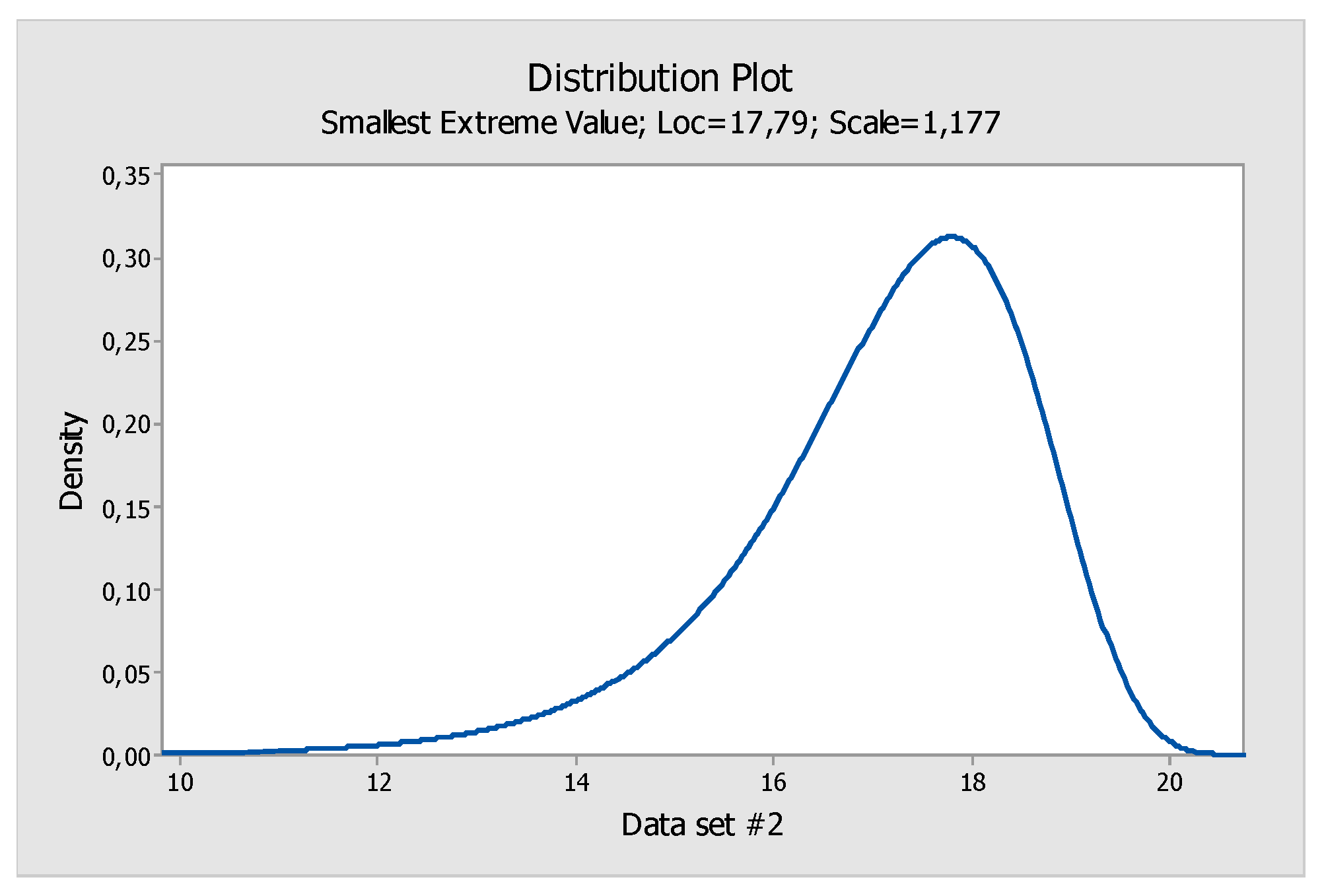
In this case study, and as an example, we chose the smallest extreme value as the best distribution fit (
Figure 6). In the case of functional depths, it is necessary to take into account that it was a data set superiorly delimited and with the probability that the data were towards the higher upper tail than towards the bottom tail. After step 1, the parameters of the fitted distribution had to be calculated (step 2).
Step 3 consisted of supplementary rules calculation. The calculation and the choice of the type
supplementary rules for Shewhart’s control charts had to be based on the magnitude of the deviation to be detected and the speed of the desired detection through the comparison of their
[
12,
13].
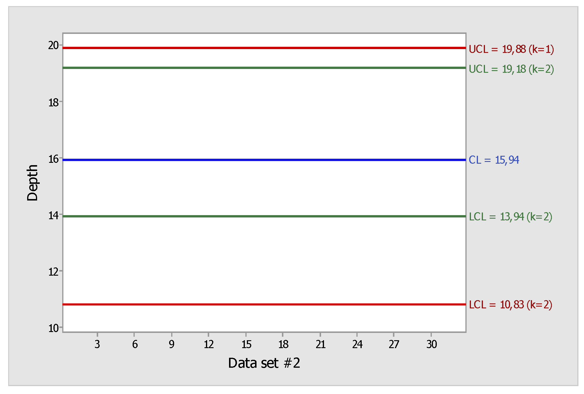
In this case, two rules, one for large deviations ( = 1) and another for small deviations ( = 2), were calculated using the solution of the general case. According to the arranged notation, the rules were referred to as and.
The following procedure was used to solve the general case of a
type rule [
2]:
Choice of the desired value.
Choice of the desired in-control value (usually = 370.4)
Calculation of the
root of the equation:
Calculation of the d control limit:
For
= 1 and in-control
= 370.4 :
After development, the polynomial was:
For
= 2 and an
value = 370.4:
Figure 7 shows the control chart with warning and control limits, and the most restrictive solution ready for last step of phase 2.
To proceed similarly to phase 2 of SPC, the chart did not include the points corresponding to the depths of the functional samples that corresponded to the chosen rational subgroups (hours, days, months, etc.) calculated according to the cut-off value obtained at the end of phase 1 of FPC.
5. Conclusions
Both: SPC and FDA and the concept of FPC can be used successfully in the search and elimination of outliers, in order to reduce any type of variability: common or random [
17,
19]. But when data do not follow a normal distribution and in auto-correlation phenomenon presence, and the false alarm rate increases [
20], FPC can be utilized effectively in the detection of outliers, also contributing major advantages in the detection of specific variability compared to traditional techniques such as Statistical Control Process [
21], even adding supplementary rules to the traditional Shewhart-type control charts. Thus, the functional approach of FPC with supplementary rules calculation, greatly enhances the capacity for analysis facilitating massive and systematic analysis of the data.
References
- J. M. J. M. 1904-2008 Juran and A. B. Godfrey, Juran’s quality handbook. New York : McGraw Hill, 1999.
- W. H. Woodall and D. C. Montgomery, “Research issues and ideas in statistical process control,” J. Qual. Technol., vol. 31, no. 4, pp. 376–386, 1999.
- W. A. Shewhart, Economic control of quality of manufactured product. New York (US): Van Nostrand Company, 1931.
- D. C. Montgomery, “Introduction to Statistical Quality Control 6th Edition with JMP(r) Version 6 Software Set.” 2008.
- C. A. Acosta-Mejia, “Two Sets of Runs Rules for the Chart,” Qual. Eng., vol. 19, no. 2, pp. 129–136, 2006.
- P. M. Berthouex, W. G. P. M. Berthouex, W. G. Hunter, and L. C. Y. Pallesen andShih, “The use of stochastic models in the interpretation of historical data from sewage treatment plants,” Water Research, vol. 10. pp. 689–698, 1976.
- L. C. Alwan and H. V. Roberts, “Time-Series Modeling for Statistical Process Control,” J. Bus. Econ. Stat., vol. 6, pp. 87–95, 1988.
- W. Electric, Western Electric’s Statistical Quality Control Handbook. 1956.
- L. S. NELSON, “The Shewhart Control Chart - Tests for Special Causes,” J. Qual. Technol., vol. 16, no. 4, pp. 237–239, 1984.
- W. B. Gartner, M. J. W. B. Gartner, M. J. Naughton, W. E. Deming, H. W. Gitlow, S. J. Gitlow, N. Mann, W. W. Scherkenbach, and M. Walton, “The Deming Management Method,” The Academy of Management Review, vol. 13. p. 138, 1988.
- J. O. Westgard, “Statistical Quality Control Procedures,” Clinics in Laboratory Medicine, vol. 33. pp. 111–124, 2013.
- C. W. Champ and W. H. Woodall, “Exact Results for Shewhart Control Charts with Supplementary Runs Rules,” Technometrics, vol. 29, no. 4, pp. 393–399, 1987.
- M. B. C. Khoo, “Design of Runs Rules Schemes,” Qual. Eng., vol. 16, no. 1, pp. 27–43, 2002.
- M. Febrero, P. M. Febrero, P. Galeano, and W. González-Manteiga, “Outlier detection in functional data by depth measures, with application to identify abnormal NOx levels,” Environmetrics, vol. 19, no. 4, pp. 331–345, 2008.
- B. W. Silverman and J. O. Ramsay, Functional Data Analysis. Springer, 2005.
- Cuevas, “A partial overview of the theory of statistics with functional data,” J. Stat. Plan. Inference, vol. 147, pp. 1–23, Apr. 2014.
- J. Sancho, J. J. Sancho, J. Martínez, J. J. Pastor, J. Taboada, J. I. Piñeiro, and P. J. García-Nieto, “New methodology to determine air quality in urban areas based on runs rules for functional data,” Atmos. Environ., vol. 83, pp. 185–192, 2014.
- J. M. nez, Á. Saavedra, P. J. García-Nieto, J. I. Piñeiro, C. Iglesias, J. Taboada, J. Sancho, and J. Pastor, “Air quality parameters outliers detection using functional data analysis in the Langreo urban area (Northern Spain),” Appl. Math. Comput., vol. 241, no. C, pp. 1–10, 2014.
- J. Martínez, Á. Saavedra, P. García-Nieto, J. I. Piñeiro, C. Iglesias, J. Taboada, J. Sancho, and J. Pastor, “Air quality parameters outliers detection using functional data analysis in the Langreo urban area (Northern Spain),” Appl. Math. Comput., vol. 241, no. C, pp. 1–10, 2014.
- W. H. Woodall, “Controversies and contradictions in statistical process control - Response,” J. Qual. Technol., vol. 32, no. 4, pp. 341–350, 2000.
- J. Sancho, C. J. Sancho, C. Iglesias, J. Piñeiro, J. Martínez, J. J. Pastor, M. Araújo, and J. Taboada, “Study of Water Quality in a Spanish River Based on Statistical Process Control and Functional Data Analysis,” Math. Geosci., 1874.
|
Disclaimer/Publisher’s Note: The statements, opinions and data contained in all publications are solely those of the individual author(s) and contributor(s) and not of MDPI and/or the editor(s). MDPI and/or the editor(s) disclaim responsibility for any injury to people or property resulting from any ideas, methods, instructions or products referred to in the content. |
© 2024 by the authors. Licensee MDPI, Basel, Switzerland. This article is an open access article distributed under the terms and conditions of the Creative Commons Attribution (CC BY) license (http://creativecommons.org/licenses/by/4.0/).
