Introduction
It is customary to divide reasons for the mortality of forest trees to stand dynamics on the one hand, and external factors on the other. The internal dynamics of a stand induce a self-thinning process [
1,
2,
3], whereas external factors may induce mortality even if within-stand competition would not [
4,
5]. The self-thinning rate may greatly depend on the initial stand density, or the development stage of any stand [
4]. To account for the self-thinning process, any mortality model must contain some measure of stand density [
6,
7,
8]. Tree status contribution to mortality also appears to depend on stand status [
9]. The mortality time rate also probably depends on site fertility and other variables contributing to the forest growth rate [
1,
2,
10,
11,
12,
13]. On the other hand, the growth rate of an individual tree correlates negatively with mortality [
14]. Decrement in net primary productivity predicts increasing mortality [
15]. Aging senescence as such may contribute [
16]. Volume mortality rates are often smaller than mortality rates on stem count bases [
17].
External factors typically induce fluctuations in the mortality rate [
18]; trends in external circumstances also induce trends in tree mortality, probably interacting with stand internal dynamics [
4,
19,
20,
21,
22]. The interaction with stand dynamics induces a contribution of stand structure and relative position of any tree within the stand [
23]. Similarly, mortality allocation within any self-thinning process depends on stand structure and tree position, possibly also stand history [
2]. Thinnings accelerate wind damage [
24,
25,
26,
27,
28], whereas snow damage tends to concentrate to non-dominating trees [
25,
29].
A third view to tree mortality is the effect of severe disturbances. In the Pacific Northwest, stand-replacing disturbances have been reported due to wildfires exclusively [
30]. Recent severe disturbances in Europe have instead been due to combinations of drought and bark beetles [
31,
32,
33,
34], or windfall and bark beetles [
35,
36]. Drought-pathogen interactions have been reported from Central United States [
37]. Non-stand-replacing disturbances were divided to endogenous (pathogens and insects) and exogeneous (fire, wind, landslades) orgins, the latter appearing less frequent but more severe [
30]. However, mortality patterns, driven by endogeneous and exogeneous factors, apparently evolve over time [30b,31,32,33, 35,36,38,39,40].
Materials and Methods
Initially, 11 121 living trees were observed on 106 experimental plots, of which 2609 were Scots pine (
Pinus silvestris), 6752 Norway spruce (
Picea abies), 1214 silver birch (
Betula pendula), and 728 downy birch (
Betula pubescens). The plots were re-observed after a time interval from three to six years. Correspondingly, there were four different time intervals for mortality observation. For the four different time intervals, the number of measured trees, as well as the number of dead trees, is shown in
Table 1. One can calculate from
Table 1 that the average gross mortality rate was 12.0% for Scots pine, 10.4% for Norway spruce, 5.7% for silver birch, and 8.8% for downy birch. The annual average mortality rates, resulting from a logarithmic conversion, were 2.4% for Scots pine, 2.4% for Norway spruce, 1.2% for silver birch, and 1.9% for downy birch.
Descriptive statistics of the present material is given in
Table 2. It is found that the trees have mostly appeared in wooded stands: the mean value of basal area for any tree species is above 25, and the stem count above 1100/ha. The tree diameters indicate that even if some saplings have been included, the measured trees have mostly been of commercial size.
For any observation interval, there is a binary distribution of tree survival status. Correspondingly, a logistic regression was fitted separately for the data from any observation interval, and for any tree species. The logistic regression function parameters were fitted by minimizing the cost function
where
N is the number of observations,
is the observation outcome, and
is the mortality probability predicted by the logistic regression. The fitted logistic function was of the form
where
are independent variables, and
are coefficients to be fitted. In the most simple form, one independent variable was examined in Eq. (2), while the most complex case investigated contained three explaining variables, even though not necessarily mutually independent.
As the data contains observations with four distinct observation intervals, there is a need to unify the results. The mortality probability within a finite time interval is converted into an annual mortality probability as
where
is the time interval between observations.
Even if Eq. (3) gives annual mortalities, the results differ between the different observation intervals since the datasets differ. A master curve for any tree species, as a function of any explaining variable, can however be constructed as an appearance-frequency-weighted average of the annual mortalities from the different datasets.
There is an alternative method for the determination of mortality based on a dataset with varying observation intervals [
41]. Instead of modeling mortality, the survival probability is modeled as
where
t is the number of observation periods, and the annual survival probability is gained by raising Eq. (4) to the power of 1/
t. Then, the annual mortality estimate is given as
In addition to the mortality probability of individual trees predicted in terms of a logistic function, the loss rate of basal area due to mortality was investigated on stand level. As the accumulated loss was determined within a period from three to six years, the annual BA loss rate was determined using Eq. (3).
Results
Table 2 shows the minimized values of the cost function (1) for the logistic function (2) containing three single explaining variables, two explaining variables together, and then three explaining variables together, the three not being mutually independent. With a single explaining variable, the minimized cost function values display a qualitative ranking: stand basal area (
BA) does not provide the smallest value of the cost function in any case. The minimum cost function values with one explaining variable are distributed between tree diameter (
D) and basal area of larger trees within the stand (
BAL).
It is found from
Table 2 that as increasing the number of explaining variables always reduces the achievable minimum value of the cost function (1), the decrement is not very large. Correspondingly, depending on the purpose, any version of Eq. (2), as evaluated in
Table 2, may be useful. This fact is here utilized to demonstrate the effects of the explaining variable in terms of single-variable logistic models (2).
Table 3a.
Minimized values of the cost function (1) for four tree species and seven sets of explaining variables in Eq. (2), for a measurement interval of three years. Bolded numbers indicate the minimum values of the cost function within any group of explaining variables.
Table 3a.
Minimized values of the cost function (1) for four tree species and seven sets of explaining variables in Eq. (2), for a measurement interval of three years. Bolded numbers indicate the minimum values of the cost function within any group of explaining variables.
| Measurement Interval |
|
|
|
| 3 years |
|
Pinus |
Picea |
Betula |
Betula |
| |
Tree species |
silvestris |
abies |
pendula |
pubescens |
| Explaining variable |
1 |
2 |
3 |
4 |
| D |
|
0.04179 |
0.07725 |
0.03989 |
0.04121 |
| BA |
|
0.04108 |
0.07772 |
0.04762 |
0.03650 |
| BAL |
|
0.04031 |
0.07776 |
0.04477 |
0.03589 |
| D+BA |
|
0.03999 |
0.07725 |
0.03987 |
0.03513 |
| D+BAL |
|
0.04031 |
0.07706 |
0.03900 |
0.03242 |
| D+D^2+BA |
0.03948 |
0.07702 |
0.03932 |
0.03475 |
| D+D^2+BAL |
0.03975 |
0.07683 |
0.03791 |
0.03242 |
Table 3b.
Minimized values of the cost function (1) for four tree species and seven sets of explaining variables in Eq. (2), for a measurement interval of four years. Bolded numbers indicate the minimum values of the cost function within any group of explaining variables.
Table 3b.
Minimized values of the cost function (1) for four tree species and seven sets of explaining variables in Eq. (2), for a measurement interval of four years. Bolded numbers indicate the minimum values of the cost function within any group of explaining variables.
| Measurement Interval |
|
|
|
| 4 years |
|
Pinus |
Picea |
Betula |
Betula |
| |
Tree species |
silvestris |
abies |
pendula |
pubescens |
| Explaining variable |
1 |
2 |
3 |
4 |
| D |
|
0.10962 |
0.12640 |
0.03364 |
0.14173 |
| BA |
|
0.11101 |
0.12599 |
0.03788 |
0.14215 |
| BAL |
|
0.10754 |
0.12420 |
0.03230 |
0.13582 |
| D+BA |
|
0.10894 |
0.12594 |
0.03210 |
0.14000 |
| D+BAL |
|
0.10742 |
0.12360 |
0.03102 |
0.13542 |
| D+D^2+BA |
0.10888 |
0.12590 |
0.02953 |
0.13972 |
| D+D^2+BAL |
0.10740 |
0.12338 |
0.02926 |
0.13459 |
Table 3c.
Minimized values of the cost function (1) for four tree species and seven sets of explaining variables in Eq. (2), for a measurement interval of five years. Bolded numbers indicate the minimum values of the cost function within any group of explaining variables.
Table 3c.
Minimized values of the cost function (1) for four tree species and seven sets of explaining variables in Eq. (2), for a measurement interval of five years. Bolded numbers indicate the minimum values of the cost function within any group of explaining variables.
| Measurement Interval |
|
|
|
| 5 years |
|
Pinus |
Picea |
Betula |
Betula |
| |
Tree species |
silvestris |
abies |
pendula |
pubescens |
| Explaining variable |
1 |
2 |
3 |
4 |
| D |
|
0.12772 |
0.13962 |
0.15299 |
0.14007 |
| BA |
|
0.13415 |
0.14353 |
0.18063 |
0.15359 |
| BAL |
|
0.13442 |
0.14066 |
0.16593 |
0.14958 |
| D+BA |
|
0.12704 |
0.13933 |
0.15287 |
0.14004 |
| D+BAL |
|
0.12752 |
0.13836 |
0.15231 |
0.14000 |
| D+D^2+BA |
0.12502 |
0.13928 |
0.14967 |
0.13943 |
| D+D^2+BAL |
0.12506 |
0.13831 |
0.14947 |
0.13950 |
Table 3d.
Minimized values of the cost function (1) for four tree species and seven sets of explaining variables in Eq. (2), for a measurement interval of six years. Bolded numbers indicate the minimum values of the cost function within any group of explaining variables.
Table 3d.
Minimized values of the cost function (1) for four tree species and seven sets of explaining variables in Eq. (2), for a measurement interval of six years. Bolded numbers indicate the minimum values of the cost function within any group of explaining variables.
| Measurement Interval |
|
|
|
| 6 years |
|
Pinus |
Picea |
Betula |
Betula |
| |
Tree species |
silvestris |
abies |
pendula |
pubescens |
| Explaining variable |
1 |
2 |
3 |
4 |
| D |
|
0.21055 |
0.19007 |
0.11696 |
0.14206 |
| BA |
|
0.21948 |
0.19694 |
0.14221 |
0.14036 |
| BAL |
|
0.21501 |
0.19731 |
0.13644 |
0.13792 |
| D+BA |
|
0.20866 |
0.19001 |
0.10519 |
0.13889 |
| D+BAL |
|
0.20556 |
0.19000 |
0.10473 |
0.13791 |
| D+D^2+BA |
0.20750 |
0.18021 |
0.10497 |
0.13136 |
| D+D^2+BAL |
0.20462 |
0.18022 |
0.10445 |
0.12975 |
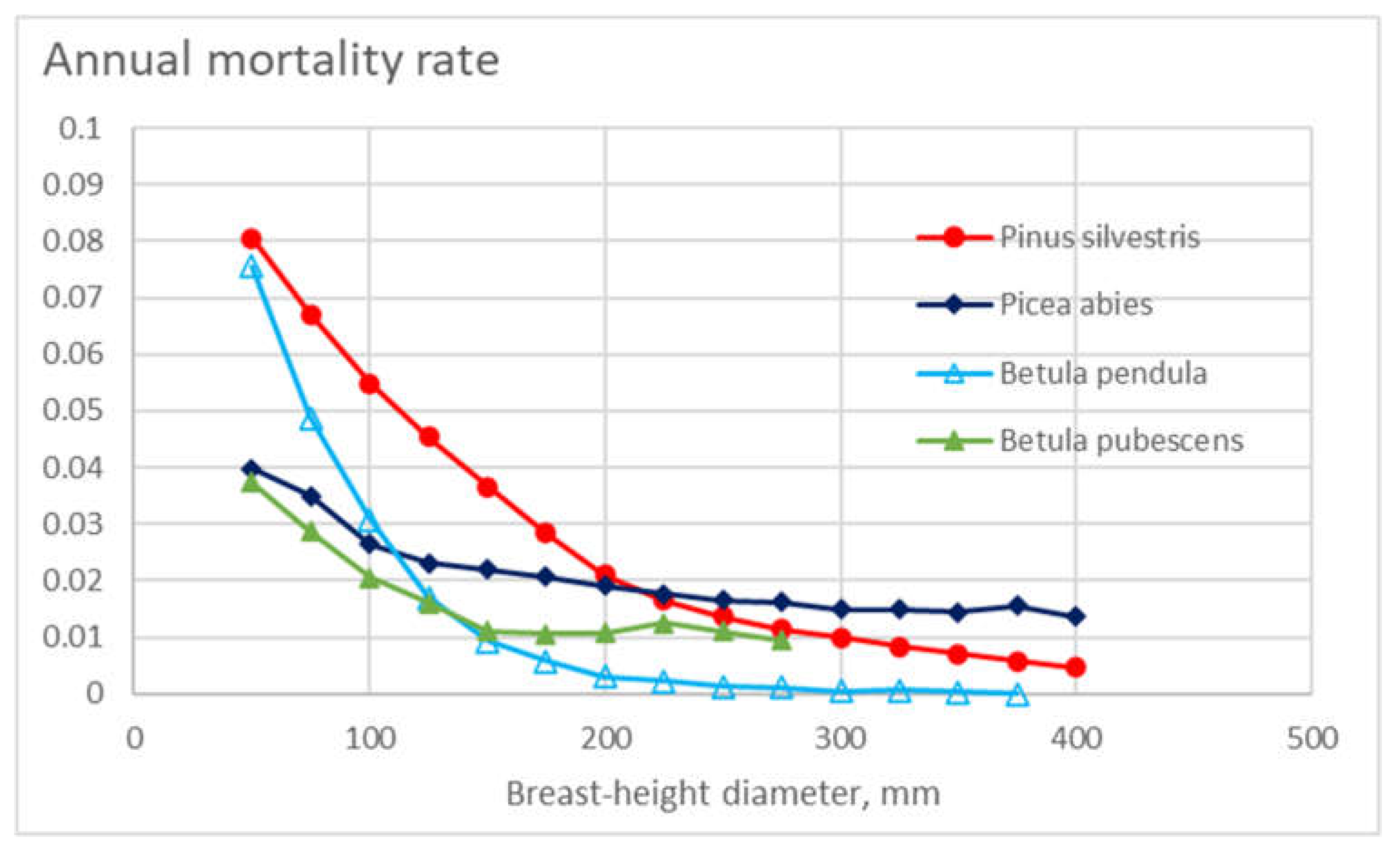
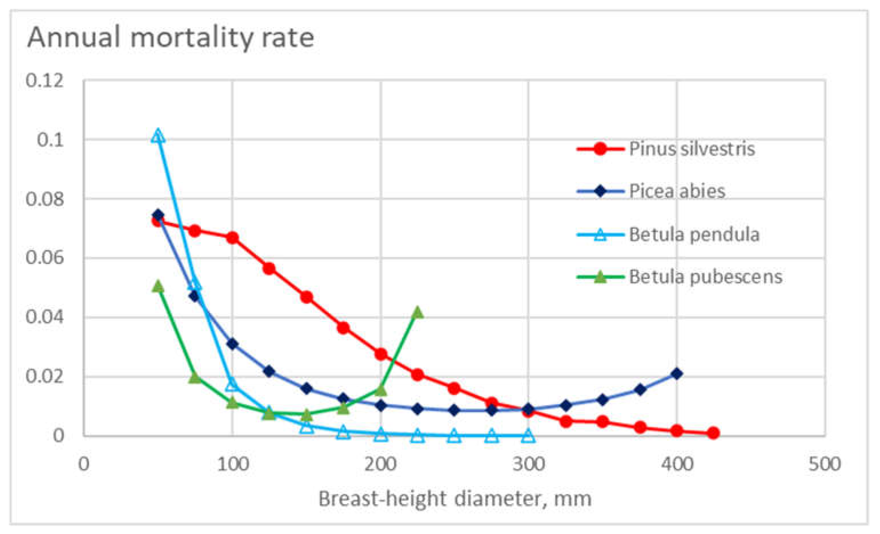
Figure 1 shows the appearance density – weighed representative master curve for annual mortality for the four tree species as a function of breast-height diameter. Generally, mortality is reduced as a function of increasing diameter. At small diameters, the mortalities of Scots pine and silver birch are the greatest. Norway spruce and downy birch are less sensitive to stem diameter, and at high diameters, the annual mortality of Norway spruce is the highest of the tree species.
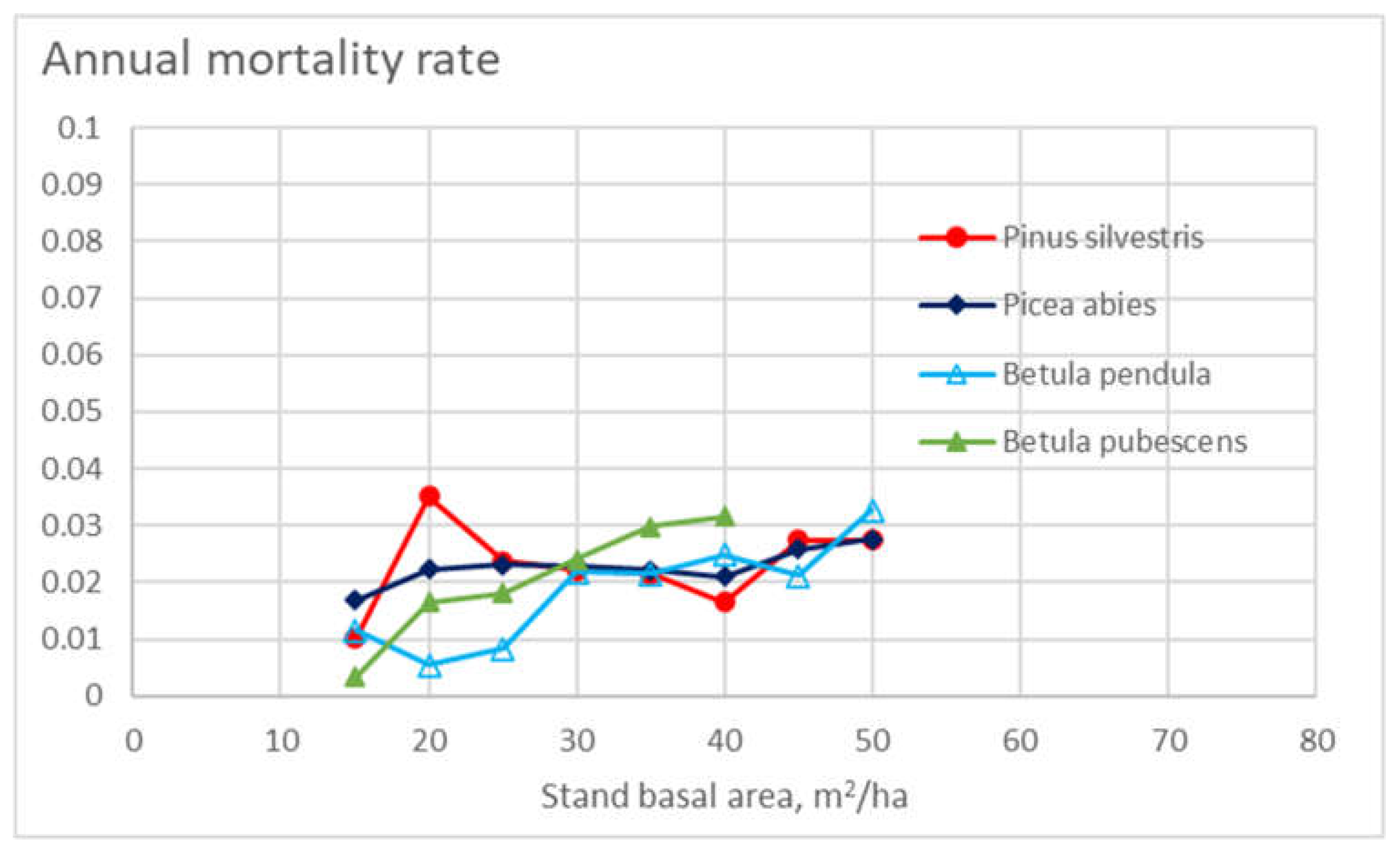
Figure 2 shows the appearance density – weighed representative master curve for annual mortality for the four tree species as a function of stand basal area. Generally, mortality is increased as a function of increasing stand basal area. The effect, however, is much weaker than that of tree diameter in
Figure 1.
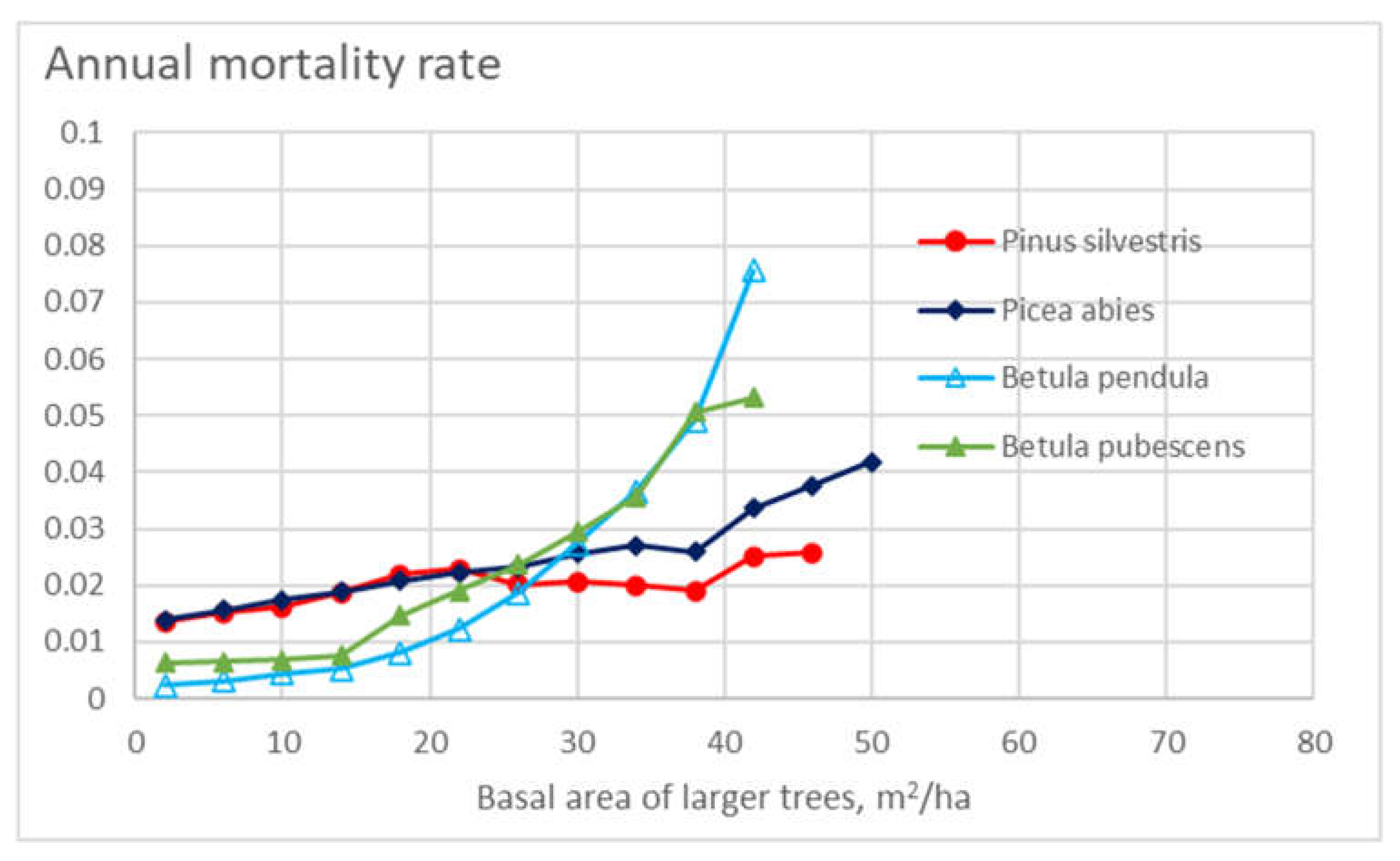
Figure 3 shows the appearance density–weight representative master curve for annual mortality for the four tree species as a function of the basal area of larger trees within the stand. Mortality increases as a function of increasing stand basal area of larger trees, and the effect is stronger than that of stand basal area in
Figure 2. In
Figure 3, the effect of the basal area of larger trees is stronger for birch species than in the case of conifers.
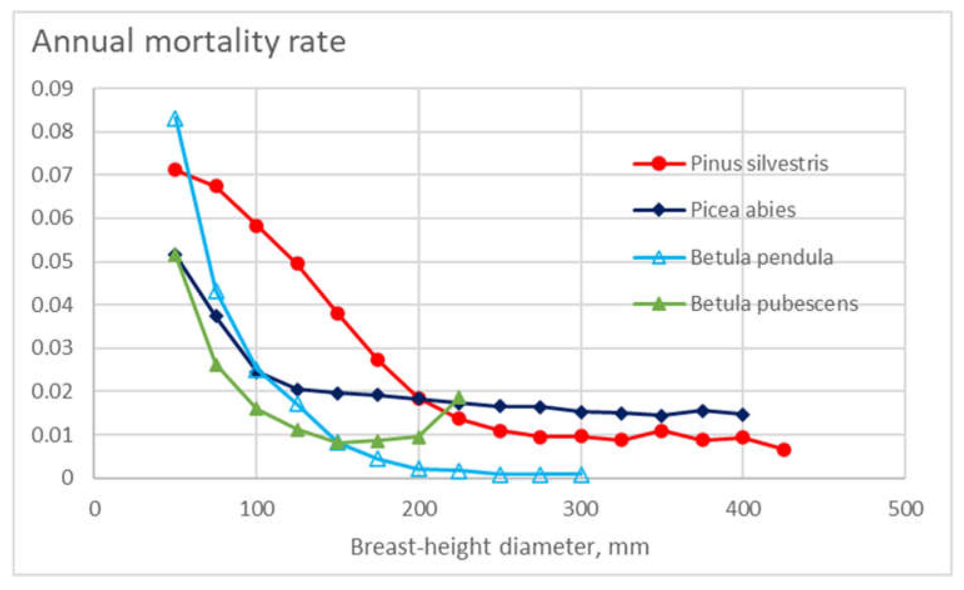
Figure 4 shows the appearance density–weight representative master curve for annual mortality for the four tree species as a function of three independent variables: the breast-height diameter, the square of the breast-height diameter, and the basal area of trees on the stand. The Figure has only one explaining variable. The squared diameter, however, is included in the modeling result (Eq. (2)). The third variable is taken as a mean-field approximation, as the expected value of the stand basal area for any tree species and breast-height diameter class. It is found that mortality decreases with increasing tree size, even if downy birch shows a non-monotonic behavior. In accordance to
Figure 1, the annual mortality of Norway spruce is the least sensitive to tree size, and at high diameters, the annual mortality of Norway spruce is the highest of the tree species.
As the results shown in
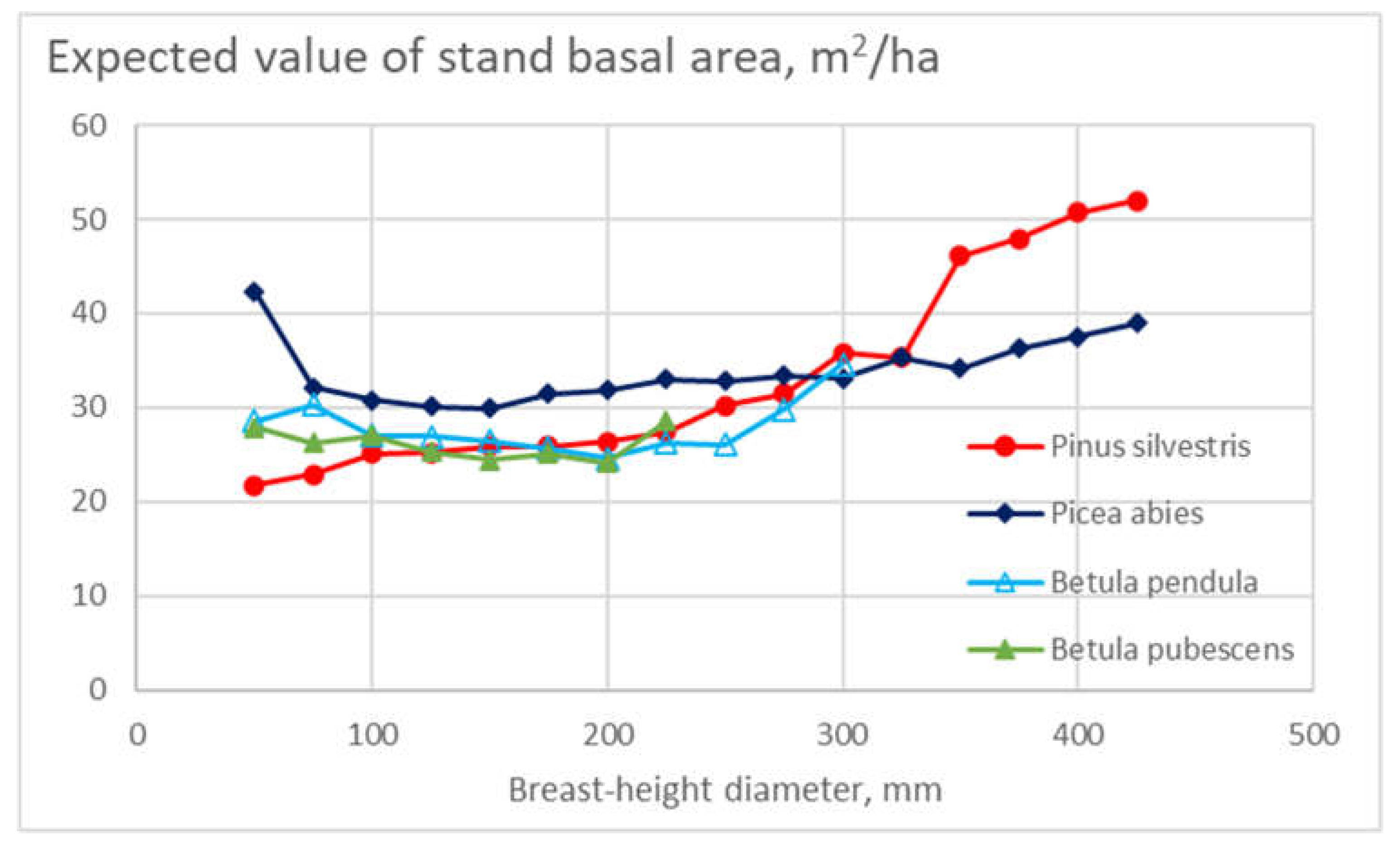
Figure 4 depend on the expected value of the stand basal area within any tree species and diameter class, the expected basal area values are of interest. They are shown in
Figure 5. It is found that the basal area expected values have been mostly below 30 m
2/ha in the case of birch species, above 30 m
2/ha in the case of spruce trees. In the case of pine trees, the basal area has increased as a function of tree size.
As the annual mortality rates were produced in Figure (4) according to Eq. (3), the alternative technique based on Eq. (5) remains to be examined. The results are shown in
Figure 6. It appears that the general level of mortalities agrees with
Figure 4, as well as the order between tree species, and most of the within-tree-species trends found in
Figure 4.
As the Eq. (5) allows the determination of the annual survival probability as a single function for any tree species, regardless of the duration of the observation periods, the coefficients of such species-specific functions (4) are worth reporting as experimental results. The coefficients are shown in
Table 4.
As the Figures above report the mortality probability of individual trees, the loss rate of basal area, commercial tree volume, or value, are of interest from the economic viewpoint.
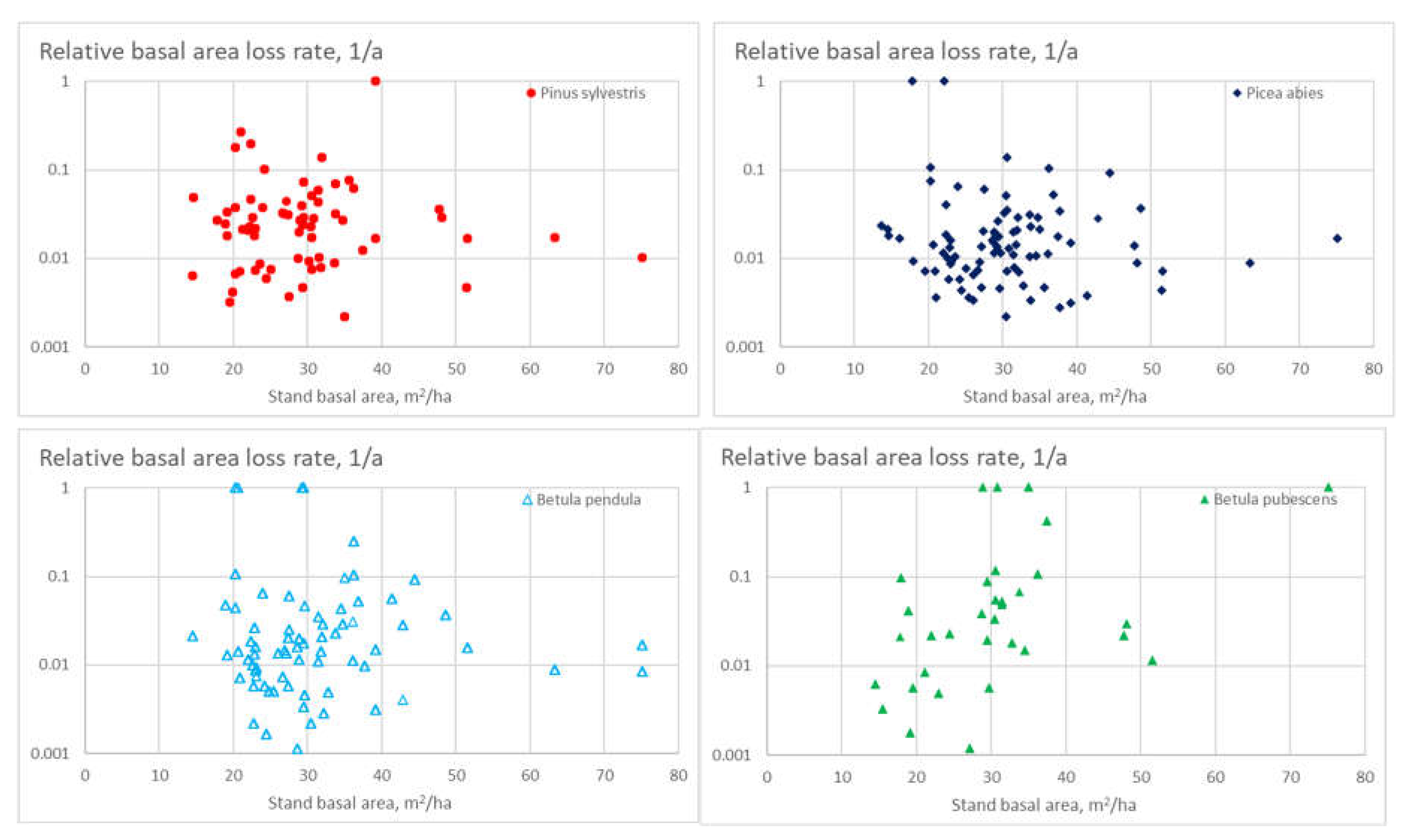
Figure 7 shows the species-specific stand-level relative basal area loss rate for the four tree species as a function of the stand basal area. Interestingly, only the downy birch displays a clear effect of stand basal area on the BA loss rate due to mortality.
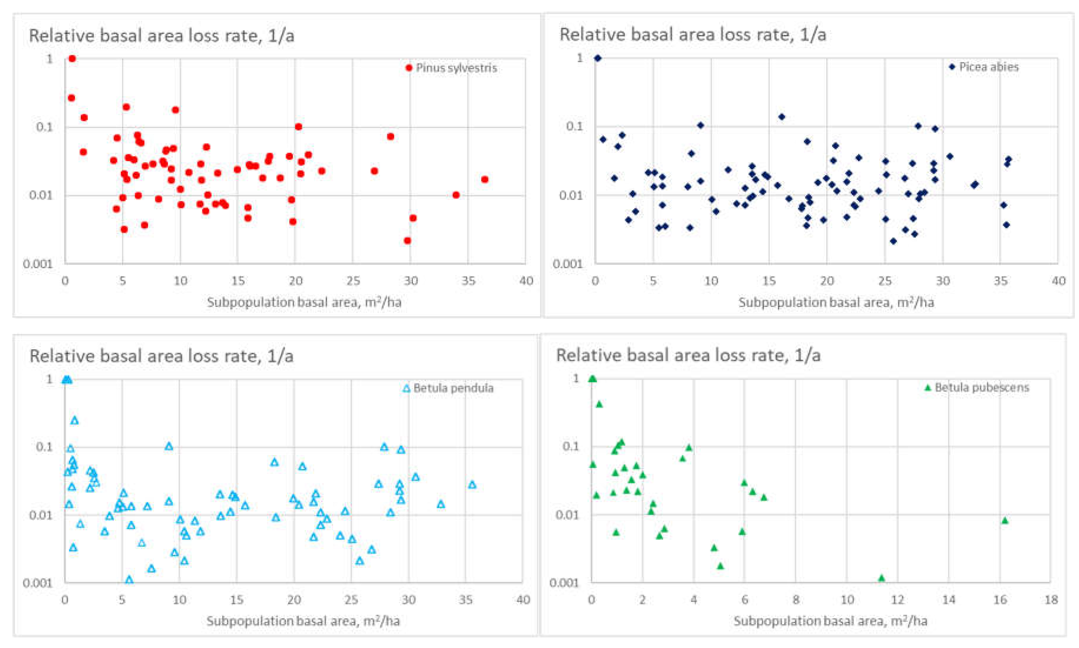
Figure 8 shows the species-specific stand-level relative basal area loss rate for the four tree species as a function of the species basal area. All the four tree species show a tendency of small minority populations dying out. Interestingly, downy birch again differs from the other tree species by showing a reduced basal area loss rate also at larger basal areas of the species.
Figure 9 shows the species-specific stand-level relative basal area loss rate for the four tree species as a function of the species basal area in relation to stand basal area. All four tree species again show the tendency of small minority populations dying out. Downy birch again differs from the other tree species by showing a reduced basal area loss rate also at larger relative basal areas of the species.
Figure 10 shows the species-specific stand-level relative basal area loss rate for the four tree species as a function of stand age. The mortality of Scots pine appears insensitive to stand age. All four tree species again show the tendency of small minority populations dying out. The mortality of Norway spruce and silver birch appear to increase with age after 100 years. Downy birch mortality increases with stand age already in the vicinity of 50 years.
Discussion
A rather interesting observation from
Figure 7 is that the basal area loss rate is insensitive to the stand basal area. A consequence is that the mortality of trees does not strongly regulate thinning practices – eventual thinnings can be designed based on other objectives but to prevent trees from dying.
Some studies have indicated mortality to increase along with basal area [
42]. The effect of stand basal area on mortality however may depend on other mortality drivers as drought, wind, snow, etc. Thinning tends to accelerate wind damage [
25]. In the present material, one driver for mortality was 2009-2010 snow damage. Basal area does not necessarily accelerate snow damage, in terms of relative basal area loss [
26,
43,
44,
45]. Apparently, snow damage probability is dominated by abiotic factors, rather than forest stand parameters [
25,
46,
47], but the tree species differ [
26,
43,
48,
49,
50].
As the gross mortality over the observation periods appeared from 6% to 12%, the level of annual mortalities in
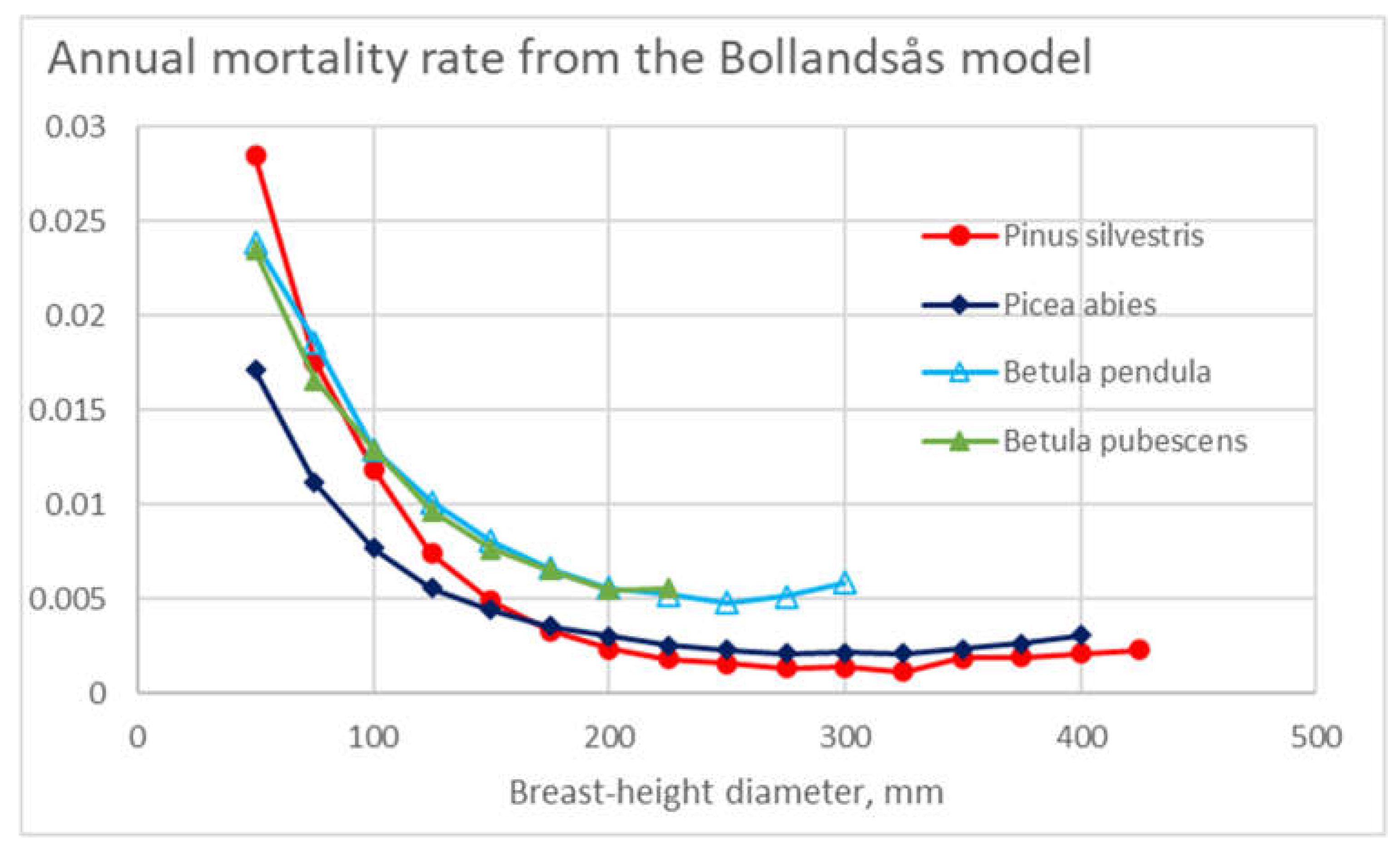
Figure 4 appears to correspond reasonably. Such mortality, however, can be compared to the outcome of models resulting from earlier investigations. The mortality model of Bollandsås [
51], parametrized for the present dataset, is shown in
Figure 11. It is found that the level of annual mortalities predicted is in the order of one third, in comparison to
Figure 4. Such a difference appears even if the expected values of stand basal areas shown in
Figure 5 are used in the model parametrization (
Figure 11).
Eventual reasons for the large difference between the models appear unknown. There may be some physical differences inducing the difference in the mortalities. One possible reason for the difference could have been snow damage during the winter 2009-2010, to some degree contributing to all observation periods of the present study. Alternatively, some modeling bias may exist. The expected value of the basal area in the data of Bollandsås has been much lower than in the present material – the model might be unable to represent the binomial mortality effect of the greater level of basal areas.
Another interesting difference is that in
Figure 11, the mortalities of birch species are greater than that of conifers. An opposite result is found from
Figure 4. The following explanation is hypothesized.
Figure 5 showing the expected values of stand basal areas at the beginning of any observation period, birch trees may have experienced a high mortality before any period of observation. Then, during any observation period, the remaining birch trees may have had a greater rate of survival. Another possible reason for the comparatively low mortality of deciduous trees is the occurrence of snow damage during leafless wintertime [
52,
53,
54].
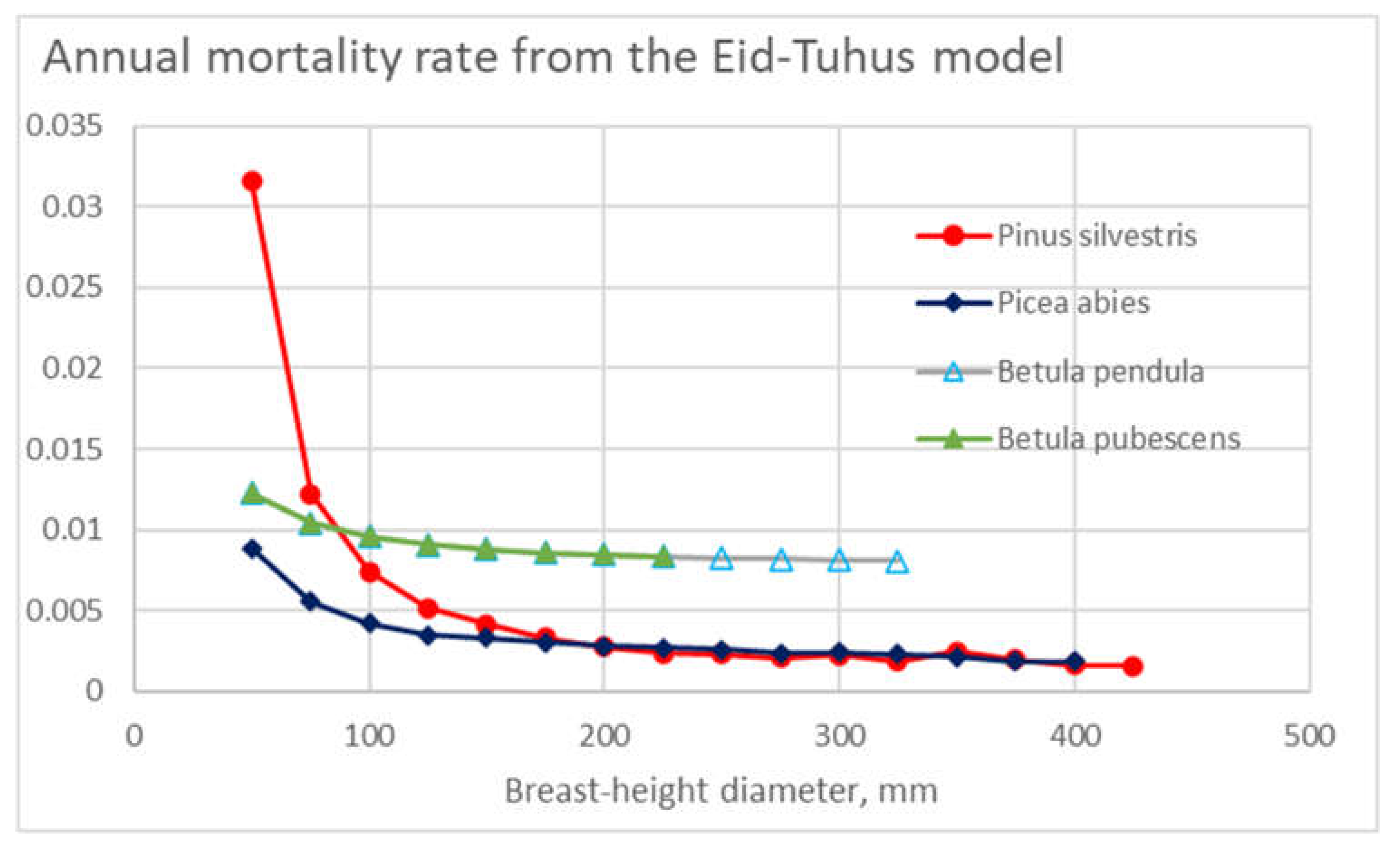
The mortality model of Eid and Tuhus [
41], parametrized for the present dataset, is shown in
Figure 12. It is found that the level of annual mortalities predicted is in the same magnitude as in the Bollandsås model (
Figure 11),
i.e. the order of one third in comparison to
Figure 4. However, in the case of three of the four tree species, the annual mortality is less dependent on tree diameter than in the case of the Bollandsås model (
Figure 11). It is not known to which degree the differences between
Figure 11 and
Figure 12 are due to different datasets and to which degree to modeling techniques [
41,
55].
A variety of mortality investigations have been published with non-boreal tree species, or with datasets from different climatic and ecological regions. Models resulting from such investigations are not necessarily transferable to the present dataset, but the magnitude of the mortality results can be compared.
The magnitude of mortalities in Germany and Switzerland, reported by Hülsmann et al [
15,
56] appear to comply with the magnitudes of
Figure 11 and
Figure 8, rather than
Figure 4 and
Figure 6, in the case of
Pinus and
Picea species, whereas mortalities reported by Etzold
et al. were higher [
39]. Similar magnitude of mortality has been reported in Eastern and Central United States [
57]. In the case of
Betula species, there is a closer compliance to
Figure 4 and
Figure 6. Mortalities in hemiboreal Estonian forests, as well as a variety of other European forests, also have had closer correspondence to
Figure 11 and
Figure 12 [
23,
58]. European fully stocked Beech and Pine forests have shown mortalities at least on the level of
Figure 4 and
Figure 6 [
59]. Boreal tree species in Belarus [
9], with stocking densities comparable to the present dataset, also have corresponded to mortalities on the level of
Figure 4 and
Figure 6.
Annual mortality in old-growth forests of Pacific Northwest has been reported [
30,
60] in the vicinity or below one percentage, in closer correspondence to
Figure 11 and
Figure 12 than to
Figure 4 and
Figure 6. Similar levels have been observed in Sierra Nevada mountains [
61]. Even smaller mortalities have been observed in Southern Pine ecosystems [
62]. Some observations, however, have indicated recently increasing mortality [30b]. In Eastern North America, conifers affected by spruce budworm defoliation have been observed mortality rates closer to those in
Figure 4 and
Figure 6 [
63].
Average annual mortality rates between 1% and 2% have been reported for East African arid woodlands [
64].
Interestingly, some qualitative patterns appearing in
Figure 4 and
Figure 6 can be compared with the literature. In the case of young trees, the mortality of Scots pine is greater than that of Norway spruce, whereas in the case of old trees, the relationship is the opposite [
23]. The mortality of Downy birch in
Figure 4 and
Figure 6 appearing to be a non-monotonic function of tree size positively corresponds to observations with a few short-lived tree species [
23,
65].
As
Figure 8 and
Figure 9 indicate that small minority species within stands tend to die out, this finding agrees with sparse literature observations [
37].
Figure 1.
Annual mortality rate in different diameter classes for the four tree species, as a function of tree diameter.
Figure 1.
Annual mortality rate in different diameter classes for the four tree species, as a function of tree diameter.
Figure 2.
Annual mortality rate in different stand classes for the four tree species, as a function of stand basal area.
Figure 2.
Annual mortality rate in different stand classes for the four tree species, as a function of stand basal area.
Figure 3.
Annual mortality rate in different stand classes for the four tree species, as a function of the basal area of larger trees on the stand.
Figure 3.
Annual mortality rate in different stand classes for the four tree species, as a function of the basal area of larger trees on the stand.
Figure 4.
Annual mortality rate in different diameter classes for the four tree species, within a model with three independent variables, where stand basal area is included as a mean-field approximation, according to Eq. (3).
Figure 4.
Annual mortality rate in different diameter classes for the four tree species, within a model with three independent variables, where stand basal area is included as a mean-field approximation, according to Eq. (3).
Figure 5.
Expected value of stand basal area in different diameter classes for the four tree species.
Figure 5.
Expected value of stand basal area in different diameter classes for the four tree species.
Figure 6.
Annual mortality rate in different diameter classes for the four tree species, within a model with three independent variables, where stand basal area is included as a mean-field approximation, according to Eq. (5).
Figure 6.
Annual mortality rate in different diameter classes for the four tree species, within a model with three independent variables, where stand basal area is included as a mean-field approximation, according to Eq. (5).
Figure 7.
Relative basal area loss rate for four tree species, as a function of stand basal area.
Figure 7.
Relative basal area loss rate for four tree species, as a function of stand basal area.
Figure 8.
Relative basal area loss rate for four tree species, as a function of species basal area.
Figure 8.
Relative basal area loss rate for four tree species, as a function of species basal area.
Figure 9.
Relative basal area loss rate for four tree species, as a function of species basal area in relation to stand basal area.
Figure 9.
Relative basal area loss rate for four tree species, as a function of species basal area in relation to stand basal area.
Figure 10.
Relative basal area loss rate for four tree species, as a function of stand age.
Figure 10.
Relative basal area loss rate for four tree species, as a function of stand age.
Figure 11.
Annual mortality rate in different diameter classes for the four tree species, plotted from the model of Bollandsås [
51], parametrized for the present dataset.
Figure 11.
Annual mortality rate in different diameter classes for the four tree species, plotted from the model of Bollandsås [
51], parametrized for the present dataset.
Figure 12.
Annual mortality rate in different diameter classes for the four tree species, plotted from the model of Eid and Tuhus [
41], parametrized for the present dataset.
Figure 12.
Annual mortality rate in different diameter classes for the four tree species, plotted from the model of Eid and Tuhus [
41], parametrized for the present dataset.
Table 1.
The number of observed trees, as well as the number of trees dying within the observation interval, for four observation intervals and four tree species.
Table 1.
The number of observed trees, as well as the number of trees dying within the observation interval, for four observation intervals and four tree species.
| Measurement Interval |
|
|
|
|
| 3 years |
|
Pinus |
Picea |
Betula |
Betula |
| |
Tree species |
silvestris |
abies |
pendula |
pubescens |
| |
Species code |
1 |
2 |
3 |
4 |
| Number of trees |
460 |
1287 |
217 |
153 |
| Number of dead trees |
9 |
58 |
5 |
3 |
| Measurement Interval |
|
|
|
|
| 4 years |
|
Pinus |
Picea |
Betula |
Betula |
| |
Tree species |
silvestris |
abies |
pendula |
pubescens |
| |
Species code |
1 |
2 |
3 |
4 |
| Number of trees |
499 |
1950 |
549 |
147 |
| Number of dead trees |
36 |
168 |
11 |
15 |
| Measurement Interval |
|
|
|
|
| 5 years |
|
Pinus |
Picea |
Betula |
Betula |
| |
Tree species |
silvestris |
abies |
pendula |
pubescens |
| |
Species code |
1 |
2 |
3 |
4 |
| Number of trees |
639 |
1855 |
171 |
184 |
| Number of dead trees |
60 |
192 |
25 |
21 |
| Measurement Interval |
|
|
|
|
| 6 years |
|
Pinus |
Picea |
Betula |
Betula |
| |
Tree species |
silvestris |
abies |
pendula |
pubescens |
| |
Species code |
1 |
2 |
3 |
4 |
| Number of trees |
1011 |
1660 |
277 |
244 |
| Number of dead trees |
208 |
282 |
28 |
25 |
| |
|
Tree |
Stand |
Basal |
Basal |
Stem |
Age |
| |
|
diameter |
basal |
area of |
area |
count |
[a] |
| |
|
[mm] |
area |
larger |
increment |
[1/ha] |
|
| |
|
|
[m2/ha] |
trees |
rate |
|
|
| |
|
|
|
[m2/ha] |
[m2/(ha*a)] |
|
| Pinus silvestris |
|
|
|
|
|
| |
min |
48 |
14.5 |
0.1 |
0.08 |
352 |
20 |
| |
max |
583 |
75.1 |
67.5 |
1.54 |
3016 |
161 |
| |
mean |
216 |
29.5 |
15.5 |
0.59 |
1160 |
60 |
| |
stdev |
86 |
11.6 |
10.4 |
0.20 |
587 |
30 |
| Picea abies |
|
|
|
|
|
|
| |
min |
24 |
14.5 |
0.0 |
0.08 |
340 |
10 |
| |
max |
996 |
75.1 |
75.1 |
1.54 |
2892 |
150 |
| |
mean |
172 |
29.5 |
22.9 |
0.59 |
1211 |
66 |
| |
stdev |
85 |
11.6 |
12.4 |
0.24 |
615 |
29 |
| Betula pendula |
|
|
|
|
|
| |
min |
29 |
13.7 |
0.1 |
0.08 |
340 |
10 |
| |
max |
459 |
75.1 |
70.6 |
1.54 |
2892 |
137 |
| |
mean |
182 |
27.5 |
17.3 |
0.57 |
1152 |
50 |
| |
stdev |
70 |
10.5 |
11.5 |
0.20 |
570 |
20 |
| Betula pubescens |
|
|
|
|
|
| |
min |
38 |
13.7 |
0.4 |
0.08 |
340 |
17 |
| |
max |
280 |
75.1 |
75.1 |
1.38 |
2711 |
132 |
| |
mean |
129 |
26.0 |
20.8 |
0.62 |
1334 |
48 |
| |
stdev |
55 |
9.4 |
9.7 |
0.19 |
660 |
17 |
Table 4.
Coefficients of Eq. (4) applied in
Figure 6.
Table 4.
Coefficients of Eq. (4) applied in
Figure 6.
| Survival model [Eq. (4)] parameters |
|
|
| |
|
Pinus |
Picea |
Betula |
Betula |
| |
Tree species |
silvestris |
abies |
pendula |
pubescens |
| Explaining variable |
1 |
2 |
3 |
4 |
| Constant |
a0 |
3.489919 |
1.297552 |
2.724741 |
1.341536 |
| D |
a1 |
-2.92E-05 |
0.025801 |
0.038834 |
0.06468 |
| D^2 |
a2 |
3.28E-05 |
-4.9E-05 |
-3.04E-05 |
-0.00023 |
| BAL |
a3 |
-0.046928 |
0.001631 |
-0.084363 |
-0.038454 |
