Eigenvalue Distributions in Random Confusion Matrices: Applications to Machine Learning Evaluation

In this paper, we derive the distribution of eigenvalues for a 2×2 random confusion matrix stemming from a machine learning (ML) evaluation problem. Additionally, we present the distributions of both the matrix’s trace and the difference between the two traces of random confusion matrices. We also illustrate the application of these derived distributions in calculating the superiority probability of four baseline ML models.

Keywords:

Subject: Computer Science and Mathematics - Probability and Statistics

MSC: 60E05; 62H30

1. Introduction

The distribution of eigenvalues of a confusion matrix is an interesting and important concept in machine learning (ML), particularly in the evaluation of classification models [1]. Confusion matrices are widely used to assess the performance of a classification algorithm by providing a detailed breakdown of the predicted and actual class labels [2]. The eigenvalues of a confusion matrix offer insights into the underlying structure and characteristics of the classification results [3,4,5]. Eigenvalues are a mathematical concept used to analyze linear transformations, and in the context of confusion matrices, they can reveal information about the matrix’s behaviour [6,7]. The distribution of eigenvalues provides a quantitative measure of the spread and concentration of information in the matrix. Understanding the distribution of eigenvalues of a confusion matrix can be valuable for various purposes, including model assessment, variable selection, high-dimensional analysis, dimension reduction, model comparison, anomaly detection, and generalization or overfitting issues [1,7,8,9,10,11].

For example, in Ref. [1], the significance of eigenvalue analysis for selecting important features in big data was explored. The authors emphasize the importance of understanding the patterns of eigenvalues in covariance matrices for various analytical purposes, such as model comparison and anomaly detection. They highlight how eigenvalues provide insights into the underlying structure of classification results, contributing to an overall understanding of model performance. In a similar study by [7], the authors utilized eigenvalue analysis in conjunction with principal component analysis (PCA) methods to reduce the dimensionality of big data before exploring the performances of several classification methods. The results of their analysis revealed that the outcomes from eigenvalue and PCA are much superior to those from the linear discriminant analysis (LDA) procedure.

In another study by [11], various eigenvalue-based dimension reduction techniques were compared for high-dimensional analysis. Specifically, the authors investigated the performances of PCA, LDA, and singular value decomposition (SVD). The findings from the study validate the utility of eigenvalue-based dimension reduction techniques in handling high-dimensional data. By comparing the effectiveness of PCA, LDA, and SVD, the research underscores the importance of eigenvalue analysis in addressing the challenges posed by high-dimensional datasets. Moreover, [12] utilized eigenvalue analysis to tackle the generalization error problem in two-layered neural networks for high-dimensional analysis. By leveraging eigenvalue properties, the study aimed to enhance the understanding of how neural networks generalize from training data to unseen data. Eigenvalue analysis in this context provides valuable insights into the behavior and performance of neural networks, particularly in high-dimensional spaces. Ref. [12] approach highlights the significance of incorporating eigenvalue-based techniques in optimizing and refining machine learning models for complex data analysis tasks.

In a different context within high-dimensional analysis, Ref. [10] employed eigenvalue and eigenvector analyses to improve the performance of high-dimensional LDA classifier in spiked covariance model. The author introduced a modified regularized R-LDA that is based on eigenvalue and eigenvector analyses. Numerical simulations, using both real and simulated data, revealed that the proposed classifier yields better classification performance than the classical R-LDA while requiring lower computational complexity. In a similar context, Ref. [9] increased the performance of support vector machine (SVM) by employing eigenvalue analysis of the features covariance matrices and subsequently performing PCA to reduce the dimension of the features. This approach helps to increase the prediction accuracy of hepatitis disease.

In a Bayesian analysis of confusion matrices, Ref. [13] delve into Bayesian methods for analyzing confusion matrices in machine learning. While Bayesian approaches are widely used in various aspects of ML, their application to confusion matrices provides a unique perspective on model evaluation. Ref. [13] provided Bayesian interpretations of various evaluation metrics derived from confusion matrices of machine learning models. The authors presented posterior distributions for these metrics from the confusion matrix and used them to compare the performances of several ML models.

The findings of various studies reviewed indicate a significant body of work on eigenvalue analysis within the context of dimension reduction, particularly in Principal Component Analysis (PCA) and Linear Discriminant Analysis (LDA). However, there is a notable gap in research concerning eigenvalue analysis of confusion matrices arising from machine learning (ML) models. In high-dimensional analysis and variable selection, dimension reduction serves as a filtering mechanism wherein techniques like eigenvalue analysis are employed to select important variables before training a classification model. Many authors, including [2,14,15,16,17,18,19,20,21], among others, have criticized this approach. They argue that it eliminates the possibility of interaction effects present in variables. Therefore, embedded and wrapper variable selection methods, which combine selection techniques and ML models, are preferred. In this regard, comparing ML models based on confusion matrices from trained model will be beneficial than covariance matrix of a pre-trained model.

Moreover, by leveraging eigenvalue analysis, researchers can objectively compare different machine learning models, discerning their relative strengths and weaknesses based on the underlying structure of their confusion matrices [22,23,24,25]. Hence, this paper presents the distribution of eigenvalues for a

2 \times 2

random confusion matrix arising from a machine learning evaluation scenario. Furthermore, we provide distributions for both the matrix’s trace and the difference between the traces of two random confusion matrices. We also demonstrate how these distributions can be utilized to compute the superiority probability of ML models.

2. Distribution of Eigenvalues of Random Confusion Matrix

Suppose we have a learning problem given by data

D = {X_{i}, Y_{i}}

, where

i \in 1, 2, \dots, n

X_{i}

is the matrix of the features, and

Y_{i}

is the response vector which we assume to be categorical with k classes. For simplicity, we consider the binary case with

k = 2

as the derivation in this paper can be easily generalized to the multiclass k classes. In any binary classification problem, the goal is to predict the

Y_{i}

based on new information

x \in X

using a classifier

\hat{y} : f (x)

. Consider a testing dataset denoted as

T = {(X_{i}, Y_{i})}_{i = 1}^{n_{T}}

, comprising

n_{T}

independent samples drawn from an unknown distribution

F (X, Y)

. To assess the accuracy of predictions made by

\hat{y}

on the samples in T, we introduce a loss function

L : y \times \hat{y} \to {a, b, c, d}

. Let y belong to

{θ_{0}, θ_{1}}

as the true class, and

\hat{y}

belong to

{θ_{0}, θ_{1}}

as the predicted class. Following convention in [13], we define the mapping of the

L

function as follows:

L = \{\begin{matrix} a, & if y = θ_{1} and \hat{y} = θ_{1} \\ b, & if y = θ_{1} and \hat{y} = θ_{0} \\ c, & if y = θ_{0} and \hat{y} = θ_{1} \\ d, & if y = θ_{0} and \hat{y} = θ_{0} \end{matrix}

(1)

where a denotes true positive, b denotes false negative, c denotes false positive and d denotes true negative. The elements of vector

L

can be presented in a

2 \times 2

matrix often referred to as a confusion matrix. Let

A

represents the

2 \times 2

confusion matrix obtained from a classification learning problem defined above;

A

can be defined as:

A = [\begin{matrix} a & b \\ c & d \end{matrix}]

(2)

The obvious properties of

A

are that (a.) it is not symmetric (b.) it is square and it is also random. Now, if we assume

A

is diagonalizable such that there exist a scalar

λ

and vector

V

that we can use to decompose

A

using

A V = λ V

(3)

then

λ = {λ_{1}, λ_{2}}

and

V = [\begin{matrix} v_{11} & v_{12} \\ v_{13} & v_{13} \end{matrix}]

are the eigenvalues and eigenvectors of

A

respectively. One interesting property of eigenvalues of this type of diagonalizable square matrix is that the sum of the eigenvalues equals the trace of the matrix. That is;

t r (A) = \sum_{j = 1}^{2} λ_{j} .

(4)

The

t r (A)

is very useful in evaluating the accuracy of a classifier in a machine learning problem most especially if the categories of the response variable is balance that is

p_{k} = 1 / k

. In a balance binary classification problem with

n_{T}

test cases, the accuracy

(\hat{ϕ})

of a classifier can be computed using:

\begin{matrix} \hat{ϕ} & = n_{T}^{- 1} t r (A) \\ = n_{T}^{- 1} \sum_{j = 1}^{2} λ_{j} . \end{matrix}

(5)

Note that, since elements of

A

are resultants of random outcomes of randomly generated test instances used to validate classifier

\hat{y}

A

can be regarded as a random matrix. Also, since only

n_{T}

is the only known parameter, the elements of

A

can be assumed to be multinomially distributed with parameters

n_{T}, π_{a}, π_{b}, π_{c}

and

π_{d}

. Thus, the joint density function of the elements in the random matrix

A

can be given as:

P (a, b, c, d | n_{T}, π_{a}, π_{b}, π_{c}, π_{d}) = \frac{n_{T}!}{a! \cdot b! \cdot c! \cdot d! \cdot} a^{π_{a}} \cdot b^{π_{b}} \cdot c^{π_{c}} \cdot d^{π_{d}} \cdot I (a + b + c + d = n_{T}) .

(6)

The last part of the RHS of (6) implies that it is required that the total sum of the four cells be equal to the number of test instances for it to be a proper pdf.

Theorem 1.

The joint probability density function (pdf) of the eigenvalues

(λ_{1}, λ_{2})

of a

2 \times 2

confusion matrix is given by:

f (λ_{1}, λ_{2}) = \frac{1}{4 s^{2} \sqrt{π}} e^{- \frac{1}{2 s^{2}} (λ_{1}^{2} + λ_{2}^{2} - 2 \bar{A} (λ_{1} + λ_{2}) + 2 {\bar{A}}^{2})} | λ_{1} - λ_{2} | - \infty \leq λ_{1}, λ_{2} \leq \infty .

(7)

Proof.

We begin this proof by standardizing the element of the confusion matrix

A

as follows:

z = s^{- 1} (A - \bar{A}),

(8)

where

\bar{A}

is the mean of all elements in

A

and

s

is the standard deviation of each element from their mean. If the confusion matrix is balanced such that

p_{k} = 1 / 4

for all four elements, the mean

\bar{A}

and standard deviation

s

are

\frac{n}{4}

and

\sqrt{\frac{3 n}{16}}

respectively. If otherwise, the mean

\bar{A}

and standard deviation

s

are computed as follows

\begin{matrix} \bar{A} & = \frac{a + b + c + d}{4}, \\ s & = \sqrt{\frac{{(a - \bar{A})}^{2} + {(b - \bar{A})}^{2} + {(c - \bar{A})}^{2} + {(d - \bar{A})}^{2}}{3}} . \end{matrix}

(9)

The next step involves the symmetrization of

z

to achieve symmetry as expected for a Gaussian Orthogonal Ensemble

(G O E)

[26,27].

z_{s} = (z + z^{T}) / 2 .

(10)

where

z_{s}

is the standardized symmetrized confusion matrix,

z

is the standardized confusion matrix and

z^{T}

is it transpose. The elements of

z_{s}

is explicitly defined as:

z_{s} = [\begin{matrix} a^{'} & b^{'} \\ b^{'} & d^{'} \end{matrix}] .

(11)

Now, that we have established that

z_{s}

is a

G O E

with joint

p d f

(a^{'}, b^{'}, d^{'})

given by

f (a^{'}, b^{'}, d^{'}) = \frac{1}{2 π} e^{- \frac{t r (z_{s}^{2})}{2}}; - \infty \leq a^{'}, b^{'}, d^{'} \leq \infty,

(12)

we can proceed to derive the distribution of eigenvalues of

z_{s}

and subsequently the distribution of eigenvalues of

A

. Note that by using the change of variable rule, the distribution of eigenvalues

(η_{1}, η_{2})

z_{s}

is given by

f (η_{1}, η_{2}) = f (a^{'}, b^{'}, d^{'}) | d e t (J) |,

(13)

where J is the change of variable Jacobian matrix. Thus, since

z_{s}

matrix is invariant under orthogonal transformation such that

z_{s} = P^{T} z_{s}^{η} P

(14)

where

P = [\begin{matrix} cos (θ) & sin (θ) \\ - sin (θ) & cos (θ) \end{matrix}]

is an orthogonal matrix and

z_{s}^{η} = [\begin{matrix} η_{1} & 0 \\ 0 & η_{2} \end{matrix}]

is a diagonal matrix of the eigenvalues of matrix

z_{s}

, we have

\begin{matrix} [\begin{matrix} a^{'} & b^{'} \\ b^{'} & d^{'} \end{matrix}] & = [\begin{matrix} cos (θ) & - sin (θ) \\ sin (θ) & cos (θ) \end{matrix}] [\begin{matrix} η_{1} & 0 \\ 0 & η_{2} \end{matrix}] [\begin{matrix} cos (θ) & sin (θ) \\ - sin (θ) & cos (θ) \end{matrix}] \\ = [\begin{matrix} η_{1} {cos}^{2} (θ) + η_{2} {sin}^{2} (θ) & (η_{1} - η_{2}) sin (θ) \\ (η_{1} - η_{2}) sin (θ) & η_{1} {sin}^{2} (θ) + η_{2} {cos}^{2} (θ) \end{matrix}] . \end{matrix}

(15)

As we’re moving from

z_{s}

z_{s}^{η}

, it is required to normalized the resultant

p d f

(η_{1}, η_{2})

using the Jacobian determinant

det (J)

. The change of variable Jacobian J is given as

\begin{matrix} J & = [\begin{matrix} \frac{\partial a^{'}}{\partial η_{1}} & \frac{\partial a^{'}}{\partial η_{2}} & \frac{\partial a^{'}}{\partial θ} \\ \frac{\partial d^{'}}{\partial η_{1}} & \frac{\partial d^{'}}{\partial η_{2}} & \frac{\partial d^{'}}{\partial θ} \\ \frac{\partial b^{'}}{\partial η_{1}} & \frac{\partial b^{'}}{\partial η_{2}} & \frac{\partial b^{'}}{\partial θ} \end{matrix}] \\ = [\begin{matrix} {cos}^{2} (θ) & {sin}^{2} (θ) & (η_{2} - η_{1}) sin (2 θ) \\ {sin}^{2} (θ) & {cos}^{2} (θ) & (η_{1} - η_{2}) sin (2 θ) \\ \frac{1}{2} sin (2 θ) & - \frac{1}{2} sin (2 θ) & (η_{1} - η_{2}) cos (2 θ) \end{matrix}] . \end{matrix}

(16)

Subsequently, the determinant of the Jacobian is given by

\begin{matrix} det (J) & = det [\begin{matrix} {cos}^{2} (θ) & {sin}^{2} (θ) & (η_{2} - η_{1}) sin (2 θ) \\ {sin}^{2} (θ) & {cos}^{2} (θ) & (η_{1} - η_{2}) sin (2 θ) \\ \frac{1}{2} sin (2 θ) & - \frac{1}{2} sin (2 θ) & (η_{1} - η_{2}) cos (2 θ) \end{matrix}] \\ = {cos}^{2} (θ) [\begin{matrix} {cos}^{2} (θ) & (η_{1} - η_{2}) sin (2 θ) \\ - \frac{1}{2} sin (2 θ) & (η_{1} - η_{2}) cos (2 θ) \end{matrix}] \\ - {sin}^{2} (θ) [\begin{matrix} {sin}^{2} (θ) & (η_{1} - η_{2}) sin (2 θ) \\ \frac{1}{2} sin (2 θ) & (η_{1} - η_{2}) cos (2 θ) \end{matrix}] \\ + (η_{2} - η_{1}) sin (2 θ) [\begin{matrix} {sin}^{2} (θ) & {cos}^{2} (θ) \\ \frac{1}{2} sin (2 θ) & - \frac{1}{2} sin (2 θ) \end{matrix}] \\ = (η_{1} - η_{2}) ({cos}^{2} (2 θ) + {sin}^{2} (2 θ)) \\ = η_{1} - η_{2} . \end{matrix}

(17)

Therefore, the corresponding joint

p d f

(η_{1}, η_{2})

for matrix

z_{s}

is given by

f (η_{1}, η_{2}) = \frac{1}{4 \sqrt{π}} e^{- \frac{1}{2} (η_{1}^{2} + η_{2}^{2})} | η_{1} - η_{2} |; - \infty \leq η_{1}, η_{2} \leq \infty .

(18)

Now that we have the distribution of the eigenvalues for the transformed matrix

z_{s}

, we can obtain the distribution of eigenvalues for the required confusion matrix

A

as follows

A = s z_{s} + \bar{A} .

(19)

From (19), it can be seen that there is a one-one correspondence between matrices

A

and

z_{s}

, thus, we can define the eigenvalues of

A

as a function of eigenvalues of

z_{s}

. This implies

λ = s η + \bar{A} .

(20)

where

λ = (λ_{1}, λ_{2})

and

η = (η_{1}, η_{2})

. Therefore, the joint

p d f

of eigenvalues of

A

is given by

\begin{matrix} f (λ_{1}, λ_{2}) & = f_{η_{1}, η_{2}} (λ_{1}, λ_{2}) | \frac{d η}{d λ} | \\ = \frac{1}{4 \sqrt{π}} e^{- \frac{1}{2 s^{2}} (λ_{1}^{2} + λ_{2}^{2} - 2 \bar{A} (λ_{1} + λ_{2}) + 2 {\bar{A}}^{2})} | \frac{λ_{1} - λ_{2}}{s} | | \frac{1}{s} | \\ f (λ_{1}, λ_{2}) & = \frac{1}{4 s^{2} \sqrt{π}} e^{- \frac{1}{2 s^{2}} (λ_{1}^{2} + λ_{2}^{2} - 2 \bar{A} (λ_{1} + λ_{2}) + 2 {\bar{A}}^{2})} | λ_{1} - λ_{2} |; - \infty \leq λ_{1}, λ_{2} \leq \infty, \end{matrix}

(21)

where

η_{1}^{2} + η_{2}^{2} = {(\frac{λ_{1} - \bar{A}}{s})}^{2} + {(\frac{λ_{2} - \bar{A}}{s})}^{2}

η_{1} - η_{2} = (\frac{λ_{1} - \bar{A}}{s}) - (\frac{λ_{2} - \bar{A}}{s})

and

\frac{d η}{d λ} = \frac{1}{s}

□

Remark 1.

Equation (21) implies

f (λ_{1}, λ_{2})

is a shifted

G O E

with mean and variance

\bar{A}

and

s^{2}

respectively.

2.1. Distribution of trace of a random confusion matrix

Theorem 2.

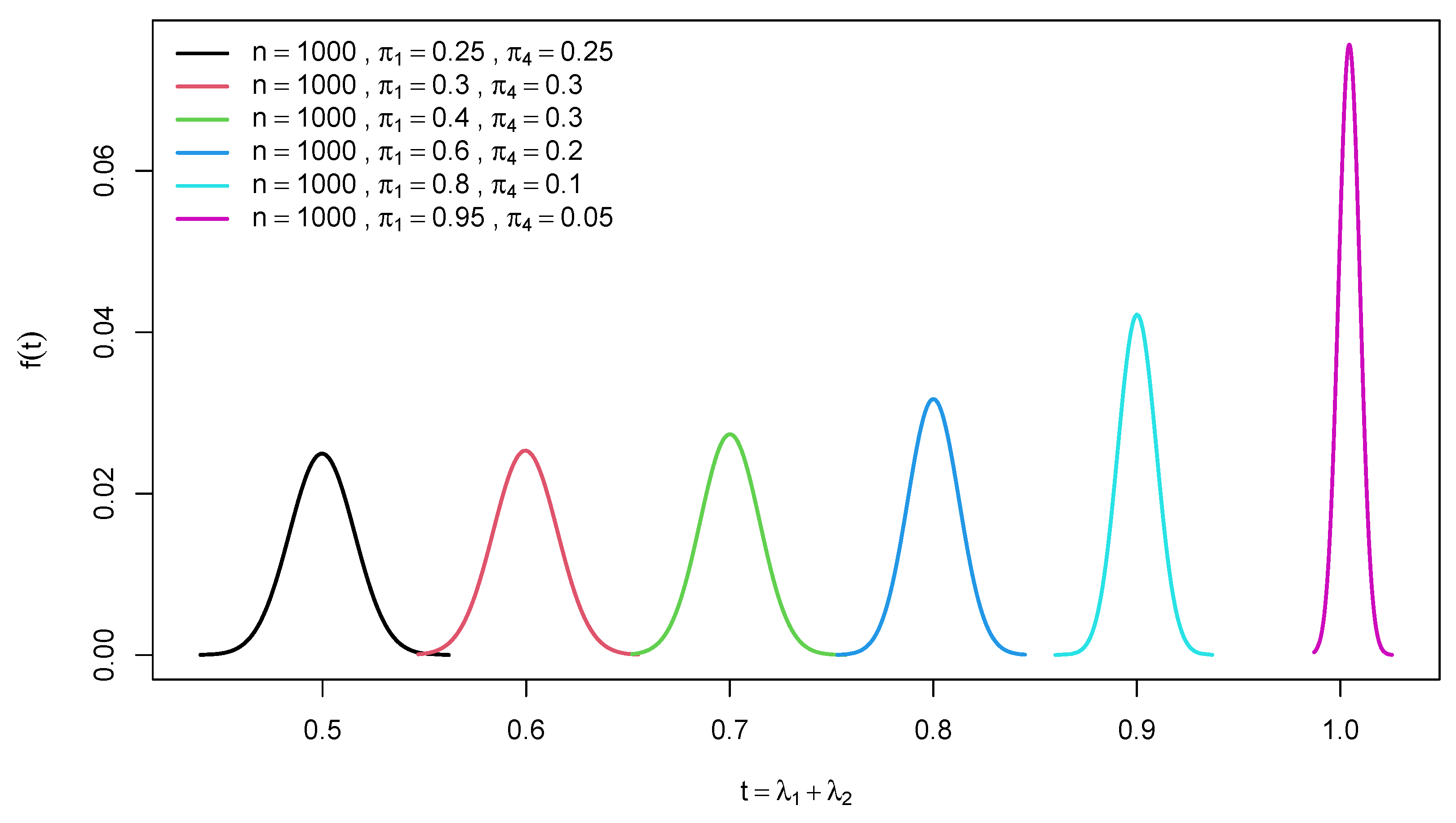
The probability density function (pdf) of the trace

t = t r (A)

of a

2 \times 2

random confusion matrix

A

is given by:

f (t) = \frac{1}{\sqrt{4 π s^{2}}} e^{- \frac{1}{4 s^{2}} {(t - 2 \bar{A})}^{2}}; - \infty \leq t \leq \infty,

(22)

Proof.

Again, considering the standardized symmetrized confusion matrix

z_{s}

defined in (11). The eigenvalues

(η_{1}, η_{2})

z_{s}

can be estimated from the characteristics equation

η^{2} - (a^{'} + d^{'}) η + (a^{'} d^{'} - b^{' 2}) = 0 .

(23)

Solving (23), gives

\begin{matrix} η_{1} & = \frac{(a^{'} + d^{'}) + \sqrt{{(a^{'} + d^{'})}^{2} - 4 b^{' 2}}}{2}, \\ η_{2} & = \frac{(a^{'} + d^{'}) - \sqrt{{(a^{'} + d^{'})}^{2} - 4 b^{' 2}}}{2} . \end{matrix}

(24)

Recall that, the trace

(w)

for matrix

z_{s}

is given by

\begin{matrix} t r (z_{s}) & = η_{1} + η_{2} \\ w & = η_{1} + η_{2} \\ = \frac{(a^{'} + d^{'}) + \sqrt{{(a^{'} + d^{'})}^{2} - 4 b^{' 2}}}{2} + \frac{(a^{'} + d^{'}) - \sqrt{{(a^{'} + d^{'})}^{2} - 4 b^{' 2}}}{2} \\ w & = a^{'} + d^{'} \end{matrix}

(25)

Lemma 1.

Suppose matrix

z_{s}

is a

G O E

, thus its elements

(a^{'}, d^{'})

are independent and identically distributed as normal,

N (0, 1)

, and

b^{'}

is distributed normally as

N (0, 1 / 2)

Remark 2.

Lemma (1) implies that the distribution of the trace of the standardized symmetrized matrix

z_{s}

is the sum of two normal distributions denoted by

N (0, 2)

. Thus,

f (w) = \frac{1}{2 \sqrt{π}} e^{- w^{2} / 4}; - \infty \leq w \leq \infty .

(26)

Again, by change of variable, we can derive the distribution of the trace of matrix

A

as follows

\begin{matrix} f (t) & = f_{w} (t) | \frac{d w}{d t} | \\ = \frac{1}{2 \sqrt{π}} e^{- (t - 2 \bar{{A)}^{2} / 4 s^{2}}} | \frac{d w}{d t} | \\ = \frac{1}{2 \sqrt{π}} e^{- {(t - 2 \bar{A})}^{2} / 4 s^{2}} | \frac{1}{s} | \\ f (t) & = \frac{1}{\sqrt{4 π s^{2}}} e^{- {(t - 2 \bar{A})}^{2} / 4 s^{2}}; - \infty \leq t \leq \infty \end{matrix}

(27)

□

Remark 3.

Equation (27) implies

f (t)

is normally distributed with mean and variance

2 \bar{A}

and

2 s^{2}

respectively and it is denoted by

N (2 \bar{A}, 2 s^{2})

Lemma 2.

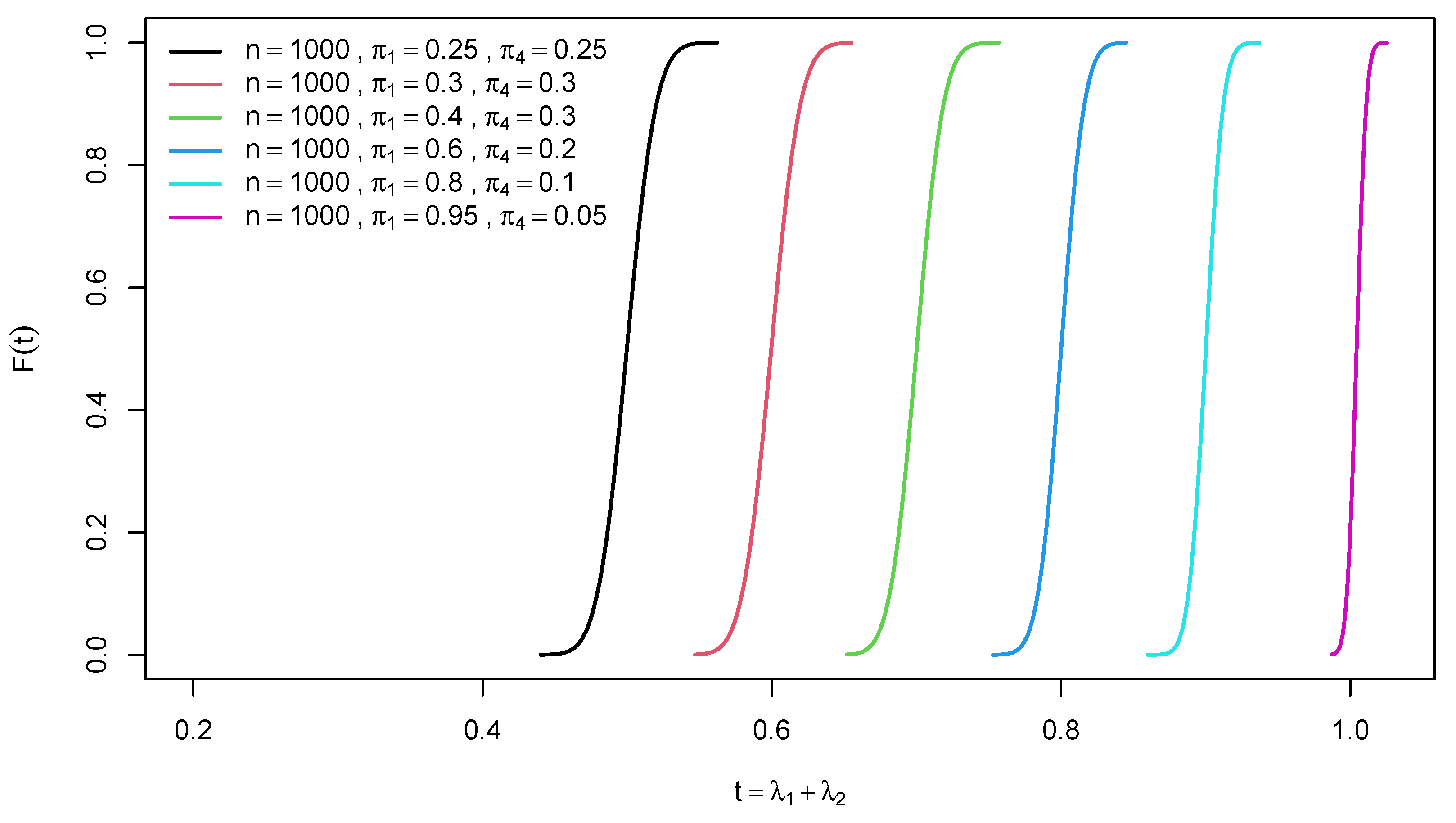
The cumulative distribution function

F (t)

for the trace of matrix

A

is given by

\begin{matrix} F (t) & = \int_{- \infty}^{t} f (t) d t \\ = \int_{- \infty}^{t} \frac{1}{\sqrt{4 π s^{2}}} e^{- {(t - 2 \bar{A})}^{2} / 4 s^{2}} d t \\ F (t) & = Φ (\frac{t - 2 \bar{A}}{\sqrt{2 s^{2}}}), \end{matrix}

(28)

where Φ is the

c d f

of standardized normal distribution with mean 0 and variance 1.

Figure 1. Graphs of the

p d f

of the trace of a random

2 \times 2

confusion matrix for different diagonal probabilities

π_{1}

and

π_{4}

Figure 1. Graphs of the

p d f

of the trace of a random

2 \times 2

confusion matrix for different diagonal probabilities

π_{1}

and

π_{4}

Figure 2. Graphs of the

c d f

of the trace of a random

2 \times 2

confusion matrix for different diagonal probabilities

π_{1}

and

π_{4}

Figure 2. Graphs of the

c d f

of the trace of a random

2 \times 2

confusion matrix for different diagonal probabilities

π_{1}

and

π_{4}

2.2. Distribution of Difference of Two Traces of Random Confusion Matrices

In machine learning, it is often valuable to compare the confusion matrices of two algorithms, such as decision trees and random forests [2,14,15]. Understanding the distribution of differences is crucial because it quantifies the degree of superiority one algorithm holds over the other. Therefore, in this section, we have developed the distribution of differences between two sets of

2 \times 2

random confusion matrices.

Theorem 3.

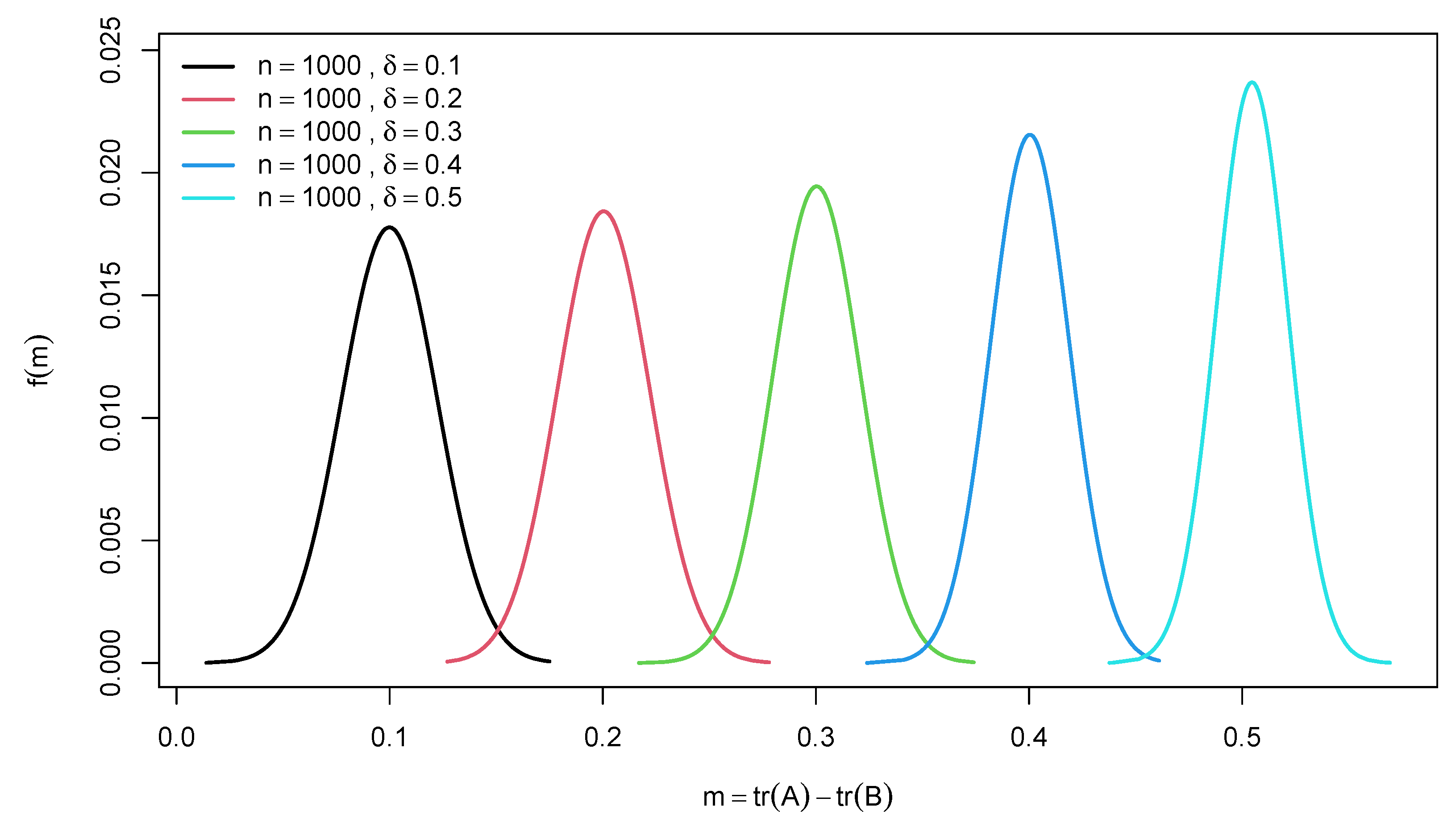
The probability density function

(p d f)

of the difference of two traces of

2 \times 2

random confusion matrices

A

and

B

denoted by

m = t r (A) - t r (B)

is given by:

f (m) = \frac{1}{\sqrt{4 π S_{A + B}^{2}}} e^{- \frac{1}{4 S_{A + B}^{2}} {(m - 2 \bar{A} + 2 \bar{B})}^{2}}; - \infty \leq m \leq \infty,

(29)

where

S_{A + B}^{2} = S_{A}^{2} + S_{B}^{2}

Proof.

This proof follows from the earlier distribution of t which follows

N (2 \bar{A}, 2 s^{2})

Lemma 3.

Suppose the traces of matrices

A

and

B

are independently distributed normal

N (2 \bar{A}, 2 s^{2})

, then the distribution of their difference is also normal with mean

2 \bar{A} - 2 \bar{B}

and variance

S_{A + B}^{2} = S_{A}^{2} + S_{B}^{2}

Remark 4.

Lemma (3) implies that the

p d f

of the difference of two traces of

2 \times 2

random confusion matrices

A

and

B

N (2 \bar{A} - 2 \bar{B}, S_{A + B}^{2})

Thus, the

p d f

of the difference of two traces of

2 \times 2

random confusion matrices

A

and

B

denoted by

m = t r (A) - t r (B)

is given by:

f (m) = \frac{1}{\sqrt{4 π S_{A + B}^{2}}} e^{- \frac{1}{4 S_{A + B}^{2}} {(m - 2 \bar{A} + 2 \bar{B})}^{2}}; - \infty \leq m \leq \infty,

(30)

□

Lemma 4.

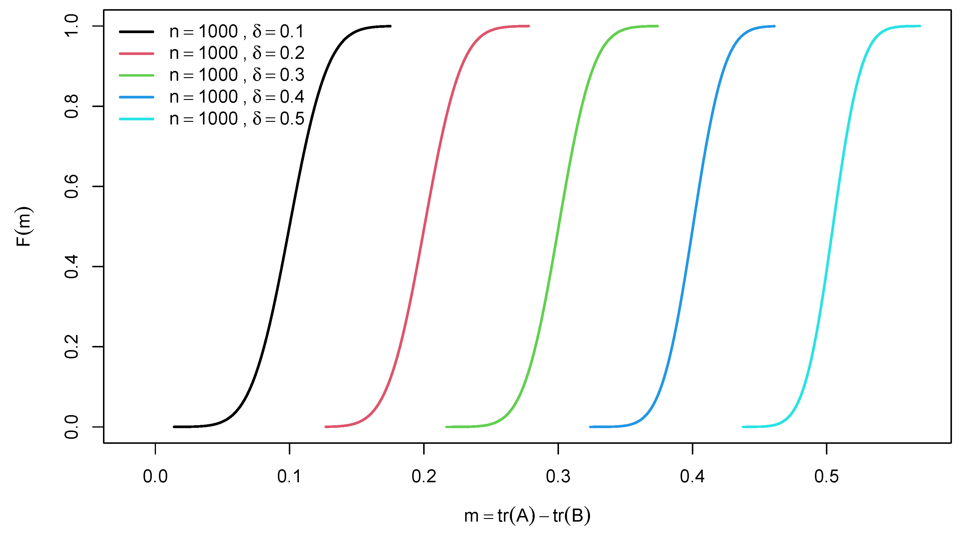
The cumulative distribution function

F (m)

for the difference of two traces of

2 \times 2

random confusion matrices

A

and

B

denoted by

m = t r (A) - t r (B)

is given by

\begin{matrix} F (m) & = \int_{- \infty}^{m} f (m) d m \\ = \int_{- \infty}^{m} \frac{1}{\sqrt{4 π S_{A + B}^{2}}} e^{- \frac{1}{4 S_{A + B}^{2}} {(m - 2 \bar{A} + 2 \bar{B})}^{2}} d m \\ F (m) & = Φ (\frac{m - 2 \bar{A} + 2 \bar{B}}{\sqrt{S_{A + B}^{2}}}), \end{matrix}

(31)

where Φ is the

c d f

of standardized normal distribution with mean 0 and variance 1.

Figure 3. Graphs of the

p d f

of for the difference of two traces of

2 \times 2

random confusion matrices for different effect size

δ = t r (A) - t r (B)

Figure 3. Graphs of the

p d f

of for the difference of two traces of

2 \times 2

random confusion matrices for different effect size

δ = t r (A) - t r (B)

Figure 4. Graphs of the

c d f

of for the difference of two traces of

2 \times 2

random confusion matrices for different effect size

δ = t r (A) - t r (B)

Figure 4. Graphs of the

c d f

of for the difference of two traces of

2 \times 2

random confusion matrices for different effect size

δ = t r (A) - t r (B)

3. Example

To demonstrate our approach, let’s examine an example featuring two classifiers, A and B, generating the following confusion matrices on the identical testing dataset T, where the size of T is

n_{T} = 200

\begin{matrix} A & = [\begin{matrix} 62 & 36 \\ 51 & 51 \end{matrix}] \\ B & = [\begin{matrix} 50 & 53 \\ 50 & 47 \end{matrix}] . \end{matrix}

(32)

The eigenvalues of matrices

A

and

B

are denoted by

(λ_{1}^{A}, λ_{2}^{A})

and

(λ_{1}^{B}, λ_{2}^{B})

respectively. Correspondingly, the traces of matrices

A

and

B

can be computed as follows:

\begin{matrix} t r (A) & = λ_{1}^{A} + λ_{2}^{A} \\ t r (B) & = λ_{1}^{B} + λ_{2}^{B} . \end{matrix}

(33)

The estimates for the eigenvalues and traces of matrices

A

and

B

are as follows:

(λ_{1}^{A} = 99.7, λ_{2}^{A} = 13.3, tr (A) = 113)

and

(λ_{1}^{B} = 100, λ_{2}^{B} = - 3, tr (B) = 97)

respectively. With these trace values, we can compute the accuracies of the two classifiers:

(ϕ^{A} = 0.57, ϕ^{B} = 0.49)

. According to this criterion, it seems that classifier A outperforms B. However, without sufficient information, we cannot conclusively determine whether this superiority is genuine or merely a result of chance. By analyzing the distribution of the difference between the two traces, as shown in (30) and (31), we can quantify the extent to which classifier A is superior to classifier B. Therefore, the probability that classifier A genuinely outperforms B is given by:

\begin{matrix} P [(ϕ^{A} = 0.57 - ϕ^{B} = 0.49) > 0] & = 1 - P [(ϕ^{A} = 0.57 - ϕ^{B} = 0.49) < 0] \\ = 1 - P (m \leq 0) \\ = 1 - F (m) \\ = 1 - Φ (\frac{m - 2 \bar{A} + 2 \bar{B}}{\sqrt{S_{A + B}^{2}}}) \\ = 1 - Φ (\frac{m - 0}{\sqrt{S_{A + B}^{2}}}) \\ = 1 - Φ (\frac{0.08}{\sqrt{0.0775}}) \\ = 0.8492 . \end{matrix}

(34)

This estimated probability value suggests a strong likelihood that model A significantly surpasses model B in terms of accuracy performance.

4. Applications

We utilize the following datasets to demonstrate the practical application of analyzing the distribution of differences between two traces of random confusion matrices in machine learning, particularly within the field of medicine and health:

Heart disease [28]: This dataset comprises information from 303 patients with heart disease at Cleveland Hospital, including 14 features. The objective is to determine the presence or absence of heart disease.
Breast cancer [29]: Originating from the University Medical Centre, Institute of Oncology, Ljubljana, Yugoslavia, this dataset contains data from 286 patients with breast cancer, encompassing 9 features. The goal is to predict the presence or absence of breast cancer recurrence.
Liver disease [30]: This dataset consists of 584 patient records from the NorthEast region of Andhra Pradesh, India, across 10 features. The objective is to predict whether a patient has liver disease using various biochemical markers.

The aim of this section is to implement and compare four baseline machine learning algorithms applied to these datasets: logistic regression (LR), decision trees (DT), random forest classification (RF), and XGboost classification (XG) [31]. The evaluation criterion utilized to compare the ML algorithms is accuracy. In addition, the supremacy of each of the algorithms is computed by computing the probability distribution in (31). Note that this probability can empirically be computed by bootstrapping the dataset L times and then obtaining the empirical distribution of the difference between two accuracies or traces. Thus, the approximate bootstrap estimate of (31) is

\hat{F} (m) = L^{- 1} \sum_{l = 1}^{L} (m_{l} < m),

(35)

where

L = 5000

is set as the bootstrap sample size. The significance of the approach presented in this study lies in its provision of a closed-form solution for this distribution. This solution offers a faster and more accurate method for calculating the distribution of differences between two accuracies.

Table 1 presents bootstrap accuracy estimates, denoted as

{\hat{ϕ}}_{L}

, along with their standard errors,

S E ({\hat{ϕ}}_{L})

, and accuracy estimates for eigenvalue distribution, denoted as

{\hat{ϕ}}_{λ}

, along with their standard errors,

S E ({\hat{ϕ}}_{λ})

, for the three datasets using the four baseline ML methods. The results indicate that the accuracy estimates and associated standard errors using both the bootstrap and eigenvalue distribution approaches are similar across the machine learning (ML) methods and datasets. This finding empirically validates the eigenvalue distribution approach for estimating the accuracy of an ML method based on the eigenvalue of a confusion matrix.

Table 2 presents pairwise comparison results of the accuracies of the four ML methods using both bootstrap and eigenvalue distribution approaches. Again, the estimates of the pairwise differences are similar in most cases in terms of direction (positive or negative). However, significant differences exist in the estimates of the superiority probability between the bootstrap and eigenvalue distribution approaches. On average, the results are approximately similar for positive differences but exhibit distinct differences for negative differences. The bootstrap tends to be conservative on average when the difference between the accuracies of two ML methods is negative but restrictive when the difference is positive. It is worth noting that bootstrap estimates are approximations to the distribution of the difference of ML accuracy, while the eigenvalue distribution provides the actual distribution of the difference based on Theorem (3). Thus, the results of the superiority probability obtained using the eigenvalue distribution are more reliable than bootstrap estimates, which have been reported in previous studies to have potentially biased estimates [32,33].

In terms of ML performance based on superiority probability, XG is on average better than LR and DT, while RF is on average better than XG. Thus, RF emerges as the best among the four ML methods across the three datasets in terms of prediction accuracy and superiority of accuracy on several replications of the experiment.

5. Conclusion

In conclusion, our study presents bootstrap accuracy estimates and accuracy estimates for eigenvalue distribution across various machine learning (ML) methods and datasets. The findings suggest that both approaches yield similar accuracy estimates and standard errors, validating the effectiveness of the eigenvalue distribution method for ML accuracy estimation based on confusion matrix eigenvalues. Pairwise comparison results reveal consistent estimates of differences between ML methods, yet significant variations exist in superiority probability estimates between bootstrap and eigenvalue distribution approaches. Notably, the bootstrap method tends to be conservative for negative differences and restrictive for positive ones. This underscores the importance of considering the actual distribution provided by the eigenvalue approach for more reliable superiority probability assessments.

Author Contributions

Conceptualization, O.R.O., A.R.R.A., M.R.A; methodology, O.R.O., A.R.R.A.; software, O.R.O.; validation, M.R.A, O.R.O. and A.R.R.A.; formal analysis, O.R.O.; investigation, M.R.A, O.R.O. and A.R.R.A.; resources, M.R.A. and A.R.R.A.; data curation, O.R.O.; writing—original draft preparation, O.R.O.; writing—review and editing, M.R.A, O.R.O. and A.R.R.A.; visualization, O.R.O; supervision, O.R.O.; project administration, O.R.O. All authors have read and agreed to the published version of the manuscript.

Funding

This research received no external funding.

Data Availability Statement

The authors confirm that the data supporting the findings of this study are available within the article.

Conflicts of Interest

The authors declare no conflict of interest.

References

Chen, R.C.; Dewi, C.; Huang, S.W.; Caraka, R.E. Selecting critical features for data classification based on machine learning methods. Journal of Big Data 2020, 7, 52. [Google Scholar] [CrossRef]
Olaniran, O.R.; Abdullah, M.A.A. Bayesian weighted random forest for classification of high-dimensional genomics data. Kuwait Journal of Science 2023, 50, 477–484. [Google Scholar] [CrossRef]
Koço, S.; Capponi, C. On multi-class classification through the minimization of the confusion matrix norm. Asian Conference on Machine Learning. PMLR, 2013, pp. 277–292.
García-Balboa, J.L.; Alba-Fernández, M.V.; Ariza-López, F.J.; Rodríguez-Avi, J. Analysis of thematic similarity using confusion matrices. ISPRS international journal of geo-information 2018, 7, 233. [Google Scholar] [CrossRef]
Übeyli, E.D.; Güler, İ. Features extracted by eigenvector methods for detecting variability of EEG signals. Pattern Recognition Letters 2007, 28, 592–603. [Google Scholar] [CrossRef]
Sayyad, S.; Shaikh, M.; Pandit, A.; Sonawane, D.; Anpat, S. Confusion matrix-based supervised classification using microwave SIR-C SAR satellite dataset. Recent Trends in Image Processing and Pattern Recognition: Third International Conference, RTIP2R 2020, Aurangabad, India, January 3–4, 2020, Revised Selected Papers, Part II 3. Springer, 2021, pp. 176–187.
Reddy, G.T.; Reddy, M.P.K.; Lakshmanna, K.; Kaluri, R.; Rajput, D.S.; Srivastava, G.; Baker, T. Analysis of dimensionality reduction techniques on big data. Ieee Access 2020, 8, 54776–54788. [Google Scholar] [CrossRef]
Golub, G.H.; Van Loan, C.F. Matrix computations; JHU press, 2013. [Google Scholar]
Alamsyah, A.; Fadila, T. Increased accuracy of prediction hepatitis disease using the application of principal component analysis on a support vector machine. Journal of Physics: Conference Series 2021, 1968, 012016. [Google Scholar] [CrossRef]
Sifaou, H.; Kammoun, A.; Alouini, M.S. High-dimensional linear discriminant analysis classifier for spiked covariance model. Journal of Machine Learning Research 2020, 21, 1–24. [Google Scholar]
Hasan, S.N.S.; Jamil, N.W. A Comparative Study of Hybrid Dimension Reduction Techniques to Enhance the Classification of High-Dimensional Microarray Data. 2023 IEEE 11th Conference on Systems, Process & Control (ICSPC). IEEE, 2023, pp. 240–245.
Lu, J.; Lu, Y. A priori generalization error analysis of two-layer neural networks for solving high dimensional Schrödinger eigenvalue problems. Communications of the American Mathematical Society 2022, 2, 1–21. [Google Scholar] [CrossRef]
Caelen, O. A Bayesian interpretation of the confusion matrix. Annals of Mathematics and Artificial Intelligence 2017, 81, 429–450. [Google Scholar] [CrossRef]
Olaniran, O.R.; Alzahrani, A.R.R. On the Oracle Properties of Bayesian Random Forest for Sparse High-Dimensional Gaussian Regression. Mathematics 2023, 11, 4957. [Google Scholar] [CrossRef]
Olaniran, O.; Abdullah, M. Subset selection in high-dimensional genomic data using hybrid variational Bayes and bootstrap priors. Journal of Physics: Conference Series. IOP Publishing, 2020, Vol. 1489, p. 012030.
Pudjihartono, N.; Fadason, T.; Kempa-Liehr, A.W.; O’Sullivan, J.M. A review of feature selection methods for machine learning-based disease risk prediction. Frontiers in Bioinformatics 2022, 2, 927312. [Google Scholar] [CrossRef] [PubMed]
Mehmood, T.; Sæbø, S.; Liland, K.H. Comparison of variable selection methods in partial least squares regression. Journal of Chemometrics 2020, 34, e3226. [Google Scholar] [CrossRef]
Chen, C.W.; Tsai, Y.H.; Chang, F.R.; Lin, W.C. Ensemble feature selection in medical datasets: Combining filter, wrapper, and embedded feature selection results. Expert Systems 2020, 37, e12553. [Google Scholar] [CrossRef]
Wang, G.; Sarkar, A.; Carbonetto, P.; Stephens, M. A simple new approach to variable selection in regression, with application to genetic fine mapping. Journal of the Royal Statistical Society Series B: Statistical Methodology 2020, 82, 1273–1300. [Google Scholar] [CrossRef]
Sauerbrei, W.; Perperoglou, A.; Schmid, M.; Abrahamowicz, M.; Becher, H.; Binder, H.; Dunkler, D.; Harrell, F.E.; Royston, P.; Heinze, G.; others. State of the art in selection of variables and functional forms in multivariable analysis—outstanding issues. Diagnostic and prognostic research 2020, 4, 1–18. [Google Scholar] [CrossRef] [PubMed]
Chowdhury, M.Z.I.; Turin, T.C. Variable selection strategies and its importance in clinical prediction modelling. Family medicine and community health 2020, 8. [Google Scholar] [CrossRef] [PubMed]
Peyrache, A.; Rose, C.; Sicilia, G. Variable selection in data envelopment analysis. European Journal of Operational Research 2020, 282, 644–659. [Google Scholar] [CrossRef]
Montoya, A.K.; Edwards, M.C. The poor fit of model fit for selecting number of factors in exploratory factor analysis for scale evaluation. Educational and psychological measurement 2021, 81, 413–440. [Google Scholar] [CrossRef]
Greenacre, M.; Groenen, P.J.; Hastie, T.; d’Enza, A.I.; Markos, A.; Tuzhilina, E. Principal component analysis. Nature Reviews Methods Primers 2022, 2, 100. [Google Scholar] [CrossRef]
Popoola, J.; Yahya, W.B.; Popoola, O.; Olaniran, O.R. Generalized self-similar first order autoregressive generator (gsfo-arg) for internet traffic. Statistics, Optimization & Information Computing 2020, 8, 810–821. [Google Scholar]
Sarkar, A.; Kothiyal, M.; Kumar, S. Distribution of the ratio of two consecutive level spacings in orthogonal to unitary crossover ensembles. Physical Review E 2020, 101, 012216. [Google Scholar] [CrossRef] [PubMed]
Grimm, U.; Römer, R.A. Gaussian orthogonal ensemble for quasiperiodic tilings without unfolding: r-value statistics. Physical Review B 2021, 104, L060201. [Google Scholar] [CrossRef]
Janosi, Andras, S.W.P.M.; Detrano, R. Heart Disease. UCI Machine Learning Repository, 1988. [CrossRef]
Zwitter, M.; Soklic, M. Breast Cancer. UCI Machine Learning Repository, 1988. [CrossRef]
Ramana, B.; Venkateswarlu, N. ILPD (Indian Liver Patient Dataset). UCI Machine Learning Repository, 2012. [CrossRef]
Ding, N.; Sadeghi, P. A submodularity-based agglomerative clustering algorithm for the privacy funnel. arXiv, arXiv:1901.06629 2019.
Navarro, C.L.A.; Damen, J.A.; Takada, T.; Nijman, S.W.; Dhiman, P.; Ma, J.; Collins, G.S.; Bajpai, R.; Riley, R.D.; Moons, K.G.; others. Risk of bias in studies on prediction models developed using supervised machine learning techniques: systematic review. bmj 2021, 375. [Google Scholar]
Tantithamthavorn, C.; McIntosh, S.; Hassan, A.E.; Matsumoto, K. An empirical comparison of model validation techniques for defect prediction models. IEEE Transactions on Software Engineering 2016, 43, 1–18. [Google Scholar] [CrossRef]

Table 1. The bootstrap accuracy estimate

{\hat{ϕ}}_{L}

along with its standard error

S E ({\hat{ϕ}}_{L})

, and the accuracy estimate for eigenvalue distribution

{\hat{ϕ}}_{λ}

along with its standard error

S E ({\hat{ϕ}}_{λ})

, for the three datasets using the four baseline methods.

Table 1. The bootstrap accuracy estimate

{\hat{ϕ}}_{L}

along with its standard error

S E ({\hat{ϕ}}_{L})

, and the accuracy estimate for eigenvalue distribution

{\hat{ϕ}}_{λ}

along with its standard error

S E ({\hat{ϕ}}_{λ})

, for the three datasets using the four baseline methods.

	Heart disease		Breast cancer		Liver disease
	${\hat{ϕ}}_{L}$	${\hat{ϕ}}_{λ}$	${\hat{ϕ}}_{L}$	${\hat{ϕ}}_{λ}$	${\hat{ϕ}}_{L}$	${\hat{ϕ}}_{λ}$
Method	$(S E ({\hat{ϕ}}_{L}))$	$(S E ({\hat{ϕ}}_{λ}))$	$(S E ({\hat{ϕ}}_{L}))$	$(S E ({\hat{ϕ}}_{λ}))$	$(S E ({\hat{ϕ}}_{L}))$	$(S E ({\hat{ϕ}}_{λ}))$
LR	0.83	0.88	0.70	0.72	0.71	0.72
LR	(0.031)	(0.032)	(0.043)	(0.031)	(0.029)	(0.029)
DT	0.77	0.76	0.71	0.73	0.72	0.67
DT	(0.042)	(0.025)	(0.031)	(0.024)	(0.031)	(0.021)
RF	0.82	0.84	0.82	0.79	0.82	0.80
RF	(0.031)	(0.029)	(0.025)	(0.030)	(0.025)	(0.030)
XG	0.77	0.82	0.74	0.70	0.75	0.72
XG	(0.036)	(0.029)	(0.030)	(0.031)	(0.030)	(0.030)

Table 2. Estimates of the difference between pairwise accuracies (

\hat{m} = ϕ_{A} - ϕ_{B}

) and their respective superiority probabilities (

1 - F (\hat{m})

) using both bootstrap and eigenvalue distribution approaches across the three datasets.

Table 2. Estimates of the difference between pairwise accuracies (

\hat{m} = ϕ_{A} - ϕ_{B}

) and their respective superiority probabilities (

1 - F (\hat{m})

) using both bootstrap and eigenvalue distribution approaches across the three datasets.

	Heart disease		Breast cancer		Liver disease
	${\hat{m}}_{L}$	${\hat{m}}_{λ}$	${\hat{m}}_{L}$	${\hat{m}}_{λ}$	${\hat{m}}_{L}$	${\hat{m}}_{λ}$
Pair	$(1 - \hat{F} ({\hat{m}}_{L}))$	$(1 - F ({\hat{m}}_{λ}))$	$(1 - \hat{F} ({\hat{m}}_{L}))$	$(1 - F ({\hat{m}}_{λ}))$	$(1 - \hat{F} ({\hat{m}}_{L}))$	$(1 - F ({\hat{m}}_{λ}))$
XG - LR	-0.05	-0.06	0.04	-0.02	0.03	0.01
XG - LR	(0.058)	(0.408)	(0.855)	(0.473)	(0.835)	(0.509)
XG - RF	-0.05	-0.02	-0.08	-0.08	-0.08	-0.08
XG - RF	(0.055)	(0.468)	(0.001)	(0.367)	(0.002)	(0.375)
XG - DT	0.00	0.06	0.02	-0.03	0.02	0.05
XG - DT	(0.481)	(0.598)	(0.728)	(0.453)	(0.719)	(0.588)
LR - RF	0.01	0.04	-0.12	-0.07	-0.11	-0.08
LR - RF	(0.536)	(0.561)	(0.000)	(0.393)	(0.000)	(0.365)
LR - DT	0.06	0.11	-0.02	-0.01	-0.01	0.04
LR - DT	(0.895)	(0.685)	(0.300)	(0.481)	(0.316)	(0.579)
RF - DT	0.05	0.08	0.10	0.06	0.10	0.13
RF - DT	(0.888)	(0.629)	(0.999)	(0.595)	(0.999)	(0.715)

Disclaimer/Publisher’s Note: The statements, opinions and data contained in all publications are solely those of the individual author(s) and contributor(s) and not of MDPI and/or the editor(s). MDPI and/or the editor(s) disclaim responsibility for any injury to people or property resulting from any ideas, methods, instructions or products referred to in the content.

© 2024 by the authors. Licensee MDPI, Basel, Switzerland. This article is an open access article distributed under the terms and conditions of the Creative Commons Attribution (CC BY) license (http://creativecommons.org/licenses/by/4.0/).

Copyright: This open access article is published under a Creative Commons CC BY 4.0 license, which permit the free download, distribution, and reuse, provided that the author and preprint are cited in any reuse.

MDPI Initiatives

Important Links

Choose an area of interest and we will send you notifications of new preprints at your preferred frequency.

Disclaimer

Eigenvalue Distributions in Random Confusion Matrices: Applications to Machine Learning Evaluation

Abstract

1. Introduction

2. Distribution of Eigenvalues of Random Confusion Matrix

2.1. Distribution of trace of a random confusion matrix

2.2. Distribution of Difference of Two Traces of Random Confusion Matrices

3. Example

4. Applications

5. Conclusion

Author Contributions

Funding

Data Availability Statement

Conflicts of Interest

References

MDPI Initiatives

Important Links

Subscribe