biSAMNet: A Novel Approach in Maritime Data Completion Using Deep Learning and NLP Techniques

1. Introduction

The automatic identification system (AIS), a useful technique for maritime communication and traffic management, transmits signals ranging from every 3 seconds to several minutes, containing a plethora of information. The data are broadly classified into static information (MMSI, ship name, type, length, and width), dynamic information (time, speed, heading, real-time vessel position), voyage-related information (destination, cargo type, route plan), and safety-related information (critical weather reports and navigational warnings from shore stations). Utilizing this data enhances understanding of vessel navigation status and has wide applications in maritime fields, including collision prevention, maritime monitoring, trajectory clustering, traffic flow prediction, and ensuring maritime safety[1].

With advancements in modern navigational information systems, the volume and accessibility of AIS data have significantly expanded. This data has become a key research focus in various maritime domains. Moreover, with the evolution of disciplines like statistics, artificial intelligence, machine learning, and data mining, the application models and methodologies pertaining to AIS are diversifying, leading to an ever-growing range of applications.At the same time, we find that machine learning methods are being further integrated with the maritime domain, with the use of classical Bayesian networks being used to analyze shipping safety management issues[2] and to analyze ship grounding accidents[3], as well as to analyze the spatial and temporal associations between internal and external factors in shallow sea waters and ship collisions[4]. There is also the use of newer knowledge mapping techniques to analyze ship collisions[5]. As well as being able to play a role in the field of ship path planning, such as in NSR areas[6] and inland waterways[7].

Peel[8] have explored using variations in fishing vessel speeds to develop a hidden Markov model (HMM) for predicting vessel behavioral states. Sousa[9] developed an HMM using speed characteristics in fishing vessel AIS trajectories to distinguish between activities (fishing and non-fishing) across three vessel types, achieving notable results. Wang[10] synthesized representations of ships using recorded AIS, investigating them through spatiotemporal matrices. Other studies[11] focus on monitoring fishing activities using AIS data, creating fishing intensity maps, or applying logistic regression to categorize and determine unknown ship types [12]. There is also a growing interest in trajectory extraction and clustering, like the route prediction algorithm based on Ornstein-Uhlenbeck random processes[13].

However, the acquisition of AIS data involves steps like generation, encapsulation, transmission, reception, and decoding. Due to variables like AIS signal transmission and device discrepancies, large volumes of raw AIS data often face issues such as information gaps, errors, and duplicates[14]. For instance, while processing AIS data, the MMSI field is expected to be 9 digits long. Yet, a considerable portion of the data features non-standard MMSI lengths, complicating the retrieval of corresponding vessel information and impacting dynamic vessel control. We noted that nearly half of the AIS data could not be successfully matched with vessel information databases. Our research aims to correlate vessel trajectories with specific static information, focusing on the vessel path.

Text representation is important in the realm of natural language processing (NLP). Effectively conveying the text’s semantic meaning is fundamental for practical applications in this field. Ensuring the accurate representation of word embedding vectors to adapt to various contexts is also a prominent area of research. We have transitioned from traditional word representation methods, such as one-hot encoding and TF-IDF, which suffered from drawbacks like high vector dimensions and an inability to accurately capture text semantics. Instead, we have embraced distributed representation methods that address these issues more effectively. These methods for representing words can be broadly categorized into static and dynamic word embeddings.

Static word embeddings encompass techniques like NNLM[15], Word2vec[16,17], while dynamic word embeddings include methods like ELMo[18], GPT[19], BERT[20], among others. NNLM employs dense vectors as word embeddings, mitigating problems like vector sparsity seen in simpler word embedding representations like TF-IDF. Word2vec introduces an efficient parameterized architecture, enabling the computation of distributed embeddings even in large corpora. However, it still relies on a one-to-one relationship between the representation and the word, failing to handle polysemy.

ELMo tackles polysemy by using the entire input sequence to create token embeddings, allowing it to differentiate homophones based on context. It also offers a dynamic embedding model that can adapt to specific tasks, departing from static lookup tables. Nevertheless, this approach deviates from the conventional design principle of training artificial neural networks, which may lead to error space and reduced performance.

In contrast to ELMo, GPT employs the Transformer model[21], known for its advantages in faster parallel processing and capturing longer-distance dependencies compared to sequential models like RNN. However, GPT’s language model is unidirectional and does not consider future context.

BERT, another Transformer-based model, addresses this limitation by being a true bidirectional language model that deeply integrates features. It combines the strengths of both ELMo and GPT. Subsequently, several improved models have emerged, such as XLNet[22], which combines the generative ability of GPT and the discriminative ability of BERT, and RoBERTa[23], which focuses on enhancing BERT’s training efficiency and performance. T5[24], on the other hand, is designed to be task-agnostic and suitable for various NLP problems.

This paper suggests an approach that integrates word embedding models with deep neural network models to classify vessel trajectories. The study divides the maritime area into spatiotemporal grids and converts the original longitude and latitude coordinates of ship trajectories into text information encoded with grid sequences. Subsequently, the Word2vec network is used to train these grid point sequences, obtaining low-dimensional embedding representations. At last, the suggested biSAMNet model is employed to effectively classify ship trajectories, identifying static information like ship types. Comparative experiments are conducted, including models of CNN, RNN, and Transformer, to evaluate the classification performance.

The research’s achievements are outlined below:

• Introduction of a new method for processing vessel trajectories: This research introduces the Visvalingam-Whyatt algorithm for path compression, followed by a grid-based encoding of AIS data. This innovative approach transforms continuous vessel trajectories into discrete sequences of grid points, which are then transformed into natural language corpora.
• Utilization of traditional Word2vec methods for embedding training: Given the insufficiency of data for training a model like BERT from scratch, this study employs traditional Word2vec techniques from the field of NLP. Each grid point is treated analogously to a word, facilitating the training of static word vectors.
• Integration of vessel trajectories with NLP techniques: The research merges ship path analysis with conventional and artificial intelligence technologies, classifying the paths through supervised learning with ship types as labels. The biSAMNet model is introduced and benchmarked against various models, including RNN, CNN, and Transformer. The results demonstrate the biSAMNet’s efficacy, particularly in lower-dimensional embeddings.

2. Materials and Methods

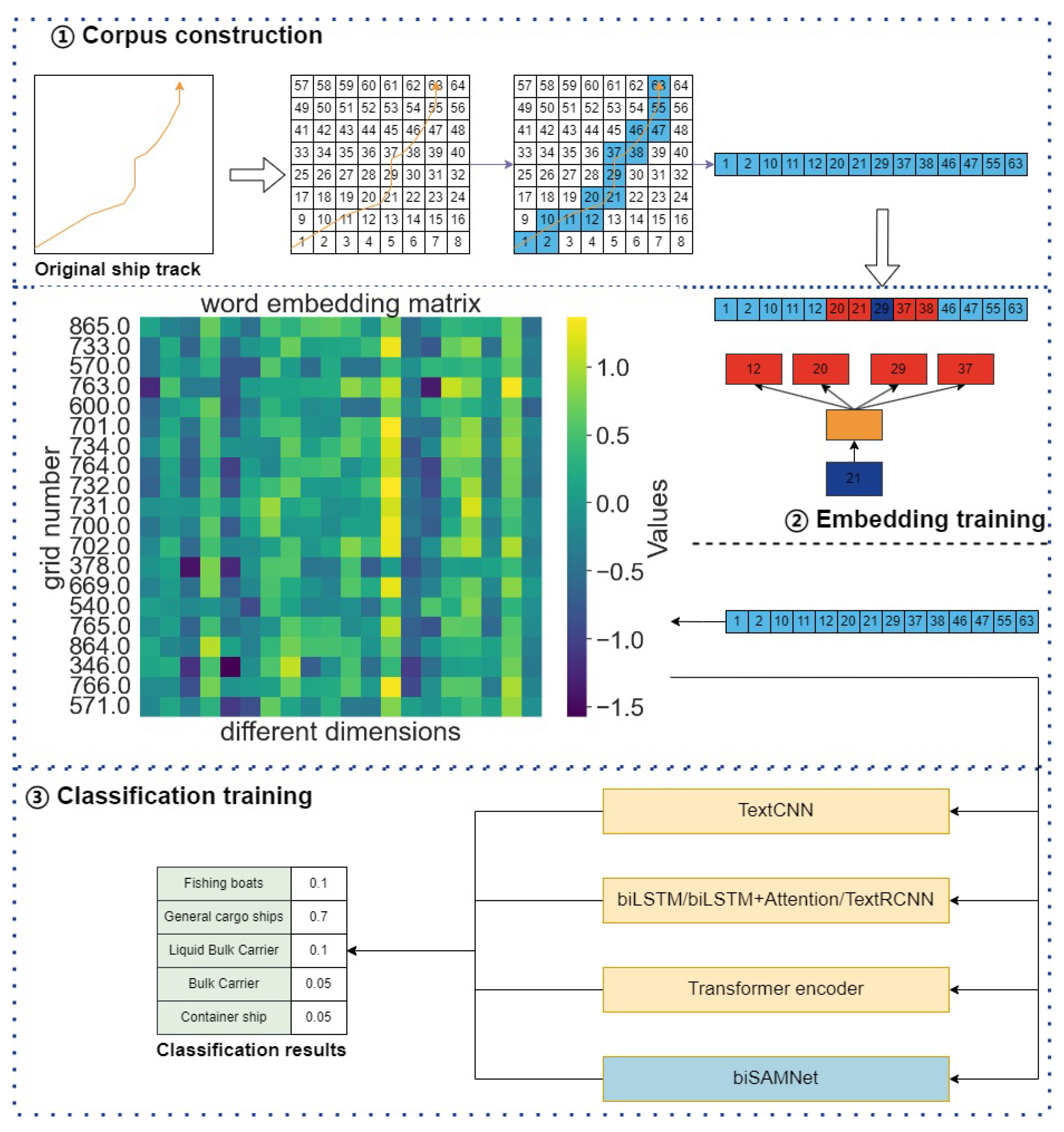
The paper proposes a hybrid approach for categorizing vessel trajectories. The particular flowchart is depicted in Figure 1, covering three phases: Corpus construction: A grid is defined within a predetermined maritime area. The original ship data (latitude and longitude) are transformed into text-like information. Embedding training: A Word2vec network is used to train the sequences of grid points, resulting in low-dimensional embedding representations. Classification training: The biSAMNet, along with CNN, RNN, Transformer, and other models, are employed to train the embedding vectors. Their performances are compared to achieve the objectives of the classification task.

2.1. Corpus Construction and Data Pretreatment Based on Grid-Coding

For vessel trajectory data (latitude and longitude), significant differences can arise even when two vessels follow identical port sequences. Unlike terrestrial traffic networks with predefined routes, maritime paths are more complex, often diverging despite proximity. To tackle this, our method employs grid encoding to standardize original data, which involves consolidating the points within the identical rectangular area into a single grid point, ensuring uniform representation of similar maritime routes.

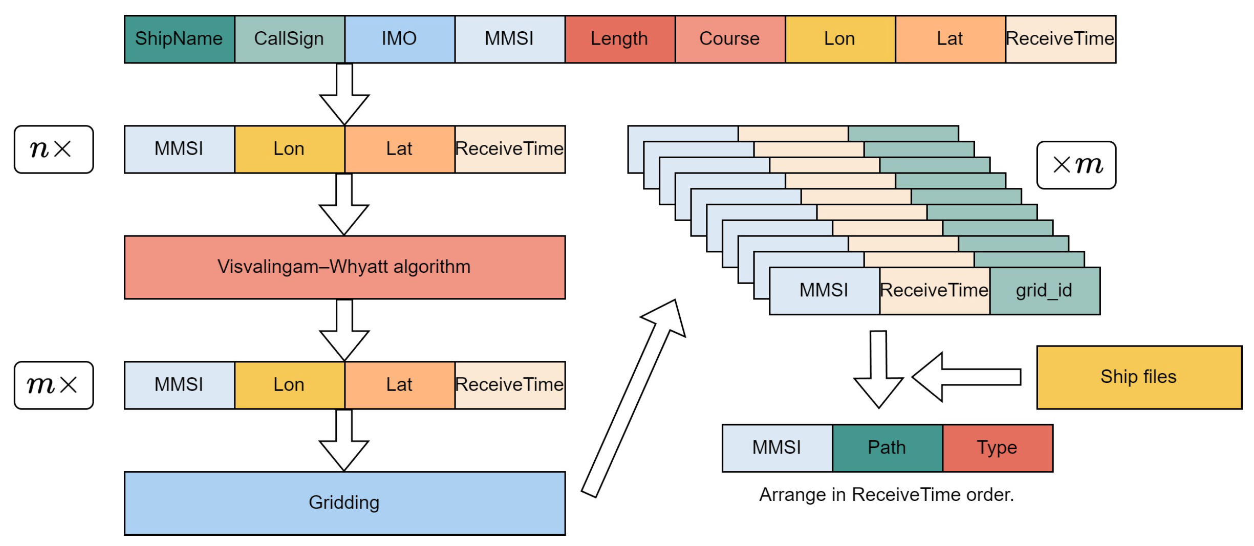
In the preprocessing stage, we retain only four fields from the original dataset: time, longitude, latitude, and MMSI, as illustrated in Table 1. Subsequently, the latitude and longitude values are transformed into their corresponding grid coordinates. Each vessel’s grid points, organized by timestamp and MMSI, undergo data compression to manage the length of the grid sequences. We utilize the Visvalingam-Whyatt algorithm for path compression. Consequently, the resulting grid sequences are of a manageable length. After processing, the data format resembles that tabulated in Table 2.

During Word2vec’s self-supervised training, exclusively the preprocessed `AllRoute’ field is used. To train the neural network classification, we implement a 30-long sliding window for subsampling the original sequences, dividing a sequence of length n into $n-30+1$ subsequences. Vessel profiles are then matched to this data to ascertain the `ShipType’ for each trajectory. Uniform processing is also applied to cases where the same `AllRoute’ corresponds to different `ShipType’ values. The entire methodology is depicted in Figure 2.

2.2. Visvalingam-Whyatt Algorithm

The Visvalingam-Whyatt algorithm is a geographic information system (GIS) algorithm designed for simplifying polygonal chains. Its fundamental principle is to minimize the number of points while preserving the key geometric characteristics of the shape. Each point within a polygonal chain is assigned an importance value based on local geometrical attributes, such as the angle at the point. Points of lesser importance are sequentially removed, determined by the area of the triangle formed by each point. Smaller areas signify lower importance, making these points candidates for removal.

What distinguishes the Visvalingam-Whyatt algorithm is its capacity to maintain the intrinsic characteristics of geographic shapes while effectively reducing point count. This reduction is vital for data storage and transmission, especially in contexts like web maps and mobile applications where resources are limited.

By decreasing point numbers in polygonal chains, the algorithm enhances the efficiency and performance of spatial data. It is particularly instrumental in GIS applications and map rendering. The Visvalingam-Whyatt algorithm, by balancing geographical shape accuracy with data volume reduction, offers an optimized solution for real-time map displays and interactive map applications. Its widespread adoption in GIS signifies its reliability and effectiveness in geographic data processing.

In the Visvalingam algorithm, the importance of each point is determined by the area of the triangle introduced by adding that point. For a series of 2D points $\left\{p_i\right\}=\left\{\left[\begin{array}{c}{x}_i\hfill \\ y_i\hfill \end{array}\right]\right\}$ , each internal point’s importance is computed according to the triangular area it forms with its immediate neighboring points. This calculation can be efficiently performed using matrix determinants or an equivalent mathematical formula (Equation 1). If the area $A_i$ of a point is below a predefined threshold p, the point is removed. This procedure is repeated iteratively until the sequence is fully traversed.

$$A_i=\frac{1}{2}|x_{i-1}{y}_i+x_i{y}_{i+1}+x_{i+1}{y}_{i-1}-x_{i-1}{y}_{i+1}-x_i{y}_{i+1}-x_{i+1}{y}_i|$$

(1)

2.3. Word Embedding Training Using Word2vec

Following the data pretreatment, we treat the processed ship trajectories as if they were natural language. To represent the discrete grid points efficaciously, we employ word embeddings and train them using the Word2Vec method on the derived corpus[17,25]. The grid point counts in vessel trajectories (868) are substantially smaller than the vocabulary size in languages like Chinese and English. Drawing inspiration from City2vec[26], we explore low-dimensional embedding techniques for this application.

Word2vec models information extraction based on the sequence of words, offering training methods of skip-gram and CBOW. In this context, let x represent a word within a sentence and y its surrounding context words. The function f represents the language model, designed to evaluate the likelihood of x and y coexisting logically in the language. The focus is not on perfecting f but rather on utilizing the intermediate parameters derived during model training as the final word vectors. Word2vec uses two acceleration techniques in training: negative sampling and hierarchical softmax.

In the skip-gram model, the objective is to utilize a word to forecast its surrounding context. A three-layer neural network is built, with words represented in their one-hot form as the input. The training objective of the neural network is to predict the correct output y for a given input x, which involves adjusting the weights from the input layer to the output layer. Usually, word embeddings have dimensions ranging from 50 to 300, whereas the input one-hot vectors are considerably larger, often in the tens of thousands. As a result, Word2Vec effectively reduces the dimensionality. In contrast, CBOW predicts the current word y using the surrounding context x.

2.4. Cosine Similarity

After obtaining low-dimensional vectors through embedding training, we aim to assess whether ship path features correlate with ship categories. Initially, we do not take into account each grid point’s sequence and utilize cosine similarity to assess similarities between various paths. This involves selecting a query path, calculating the cosine similarity with other paths, and identifying the top n paths with the highest similarity. Subsequently, we assess the proportion of these paths that fall into the same category as the query path. The methods used are as follows:

2.4.1. One-Hot Coding

Due to the manageable count of grid points (868), this approach involves directly stacking the one-hot encodings of all the grid points traversed by a vessel, without utilizing embedding results. The final vector for a path, $R_i$, is represented as shown in Equation 2, where $o_i$ is the i-th on-hot encoded grid point $e_i$ that the path passes through, and N is the total grid point count within a grid sequence.

$$R_i=\sum _{i=0}^N{o}_i{R}_i\&o_i\in {\mathbb{R}}^{868}$$

(2)

2.4.2. Word Embedding Vector Averaging

This method involves adding up and averaging word vectors from the Word2vec training results associated with a path, as depicted in Equation 3. For the experiments, embedding vectors of 50 dimensions are used.

$$R_i^{\prime }=\frac{1}{N}\sum _{i=0}^{\mathrm{N}}{e}_i{R}_i^{\prime }\&e_i\in {\mathbb{R}}^{50}$$

(3)

2.4.3. TF-IDF

This technique assesses the importance of a word in multiple documents. The word importance within a document increases with its occurrence frequency within that document. However, this importance is also influenced by the word’s frequency across the whole corpus. If a word is widespread throughout the corpus, its importance diminishes. Term frequency (TF) signifies the occurrence count of a specific word within a document. To prevent bias toward longer documents, this count is normalized by dividing it by the total term count. For a given word $t_i$ within a particular document $d_j$, its importance is represented as the score in Equation 4.

$${\mathrm{tf}}_{i,j}=\frac{n_{i,j}}{{\sum }_k{n}_{k,j}}$$

(4)

where k is the total word count within $d_j$, $n_{k,j}$ is $t_k$’s frequency within $d_j$. The numerator $n_{i,j}$ is the word frequency within $d_j$, with the denominator being the sum of frequencies of all words within $d_j$.

Inverse document frequency (IDF) quantifies a word’s overall importance. Its IDF is determined by dividing the total document count by the count of documents with that word. The result is subsequently subjected to a base-10 logarithm, as demonstrated in Equation 5.

$${\mathrm{idf}}_i=lg\frac{\left|D\right|}{\left|j:t_i\in d_j\right|}$$

(5)

where $\left|D\right|$ represents the total document count, and $|j:t_i\in d_j|$ represents the document count with the word ti (i.e., the document count where $n_{i,j}\ne 0$). In order to prevent the occurrence of division by zero, the typical approach is to incorporate the expression $1+|j:t_i\in d_j|$ in the denominator when computing the IDF value.

The word i’sTF-IDF value within $d_j$ is subsequently obtained by multiplying the word’s term frequency $t{f}_{i,j}$ in $d_j$ by its IDF value, as expressed in Equation 6.

$${\mathrm{tfidf}}_{i,j}={\mathrm{tf}}_{i,j}\times {\mathrm{idf}}_i$$

(6)

During the experiment, since we do not have access to a corpus, we regard each path as an individual document and determine the IDF values for every word within these documents. We then calculate the TF-IDF values for every grid point along the path and obtain the path’s TF-IDF average, as depicted in Equation 7.

$$R_i^{\prime \prime }=\frac{1}{N}\sum _{i=0}^N{e}_i\times {\mathrm{ifidf}}_{i,j}{R}_{\mathrm{i}}^{\prime \prime }\&e_i\in {\mathbb{R}}^{50}$$

(7)

2.5. Deep Neural Network

2.5.1. TextCNN

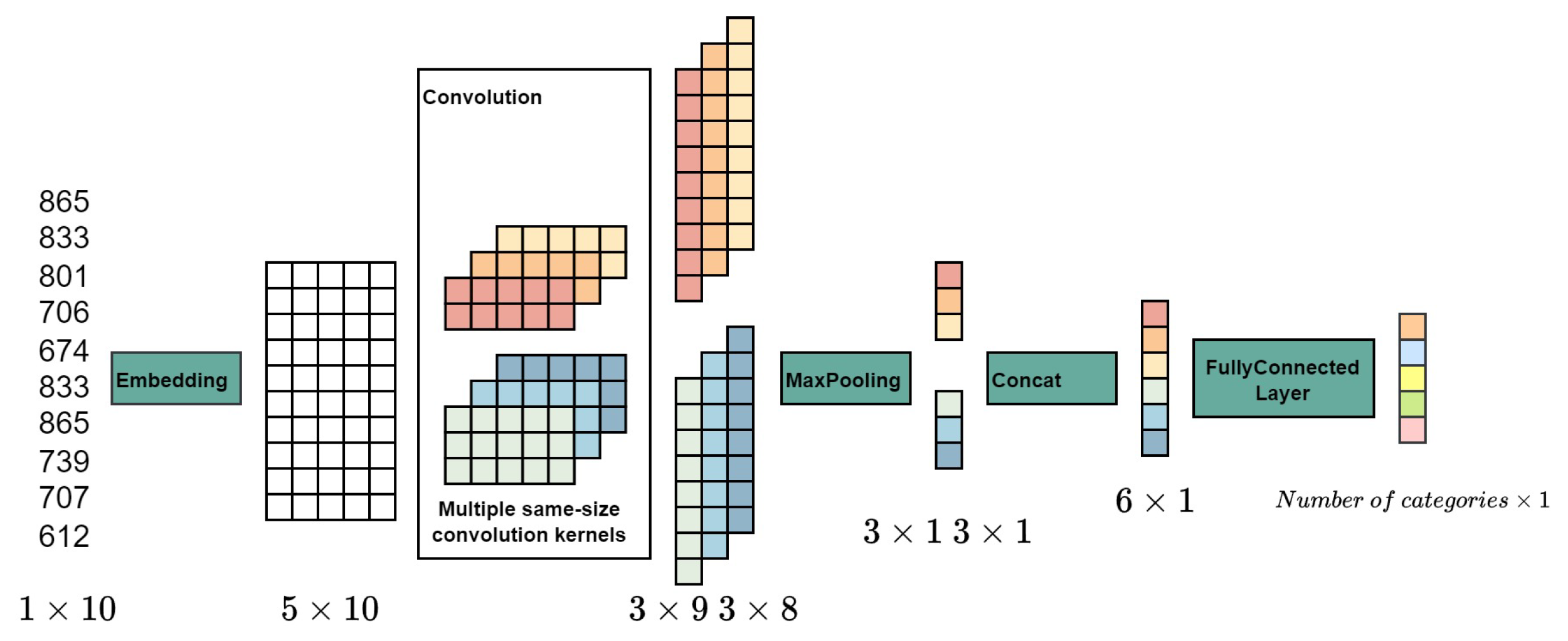
CNNs, originally designed for computer vision, have been successfully adapted for NLP tasks, particularly in text classification. TextCNN[27] represents a prominent application of CNNs in this domain, as depicted in its schematic diagram (Figure 3).

TextCNN utilizes convolutional layers to extract distinct features, applying multiple convolutional layers of various sizes. These extracted features are subsequently processed through a final linear layer to yield classification probabilities. A key aspect of TextCNN is its use of convolutional kernels of different sizes, aimed at capturing n-gram features within the text. The pooling layer, adept at managing variable sentence lengths, filters and selects pertinent features, akin to the feature engineering process in keyword extraction. $x_i\in {\mathbb{R}}_k$ means the k-dimensional word vector of the i-th word, and a n-length sentence is represented as Equation 8:

$$x_{1:n}=x_1\oplus x_2\oplus \cdots \oplus x_n$$

(8)

where ⊕ represents concatenation of vectors, forming a matrix A with dimensions $n\times k$. $x_{i,i+j}$ is defined to denote the concatenation from word i to word $i+j$. We utilize $W\in {\mathbb{R}}^{h\times k}$ to signify a convolutional kernel with a width equivalent to the word embedding dimension and a h height. This kernel operates on the matrix A, producing the feature $c_i$:

$$c_i=f(W·x_{i:i+h-1}+b)$$

(9)

where f is the activation function, and b is the bias term. The feature set obtained through multiple convolution operations is denoted as c. For each set, we use max pooling $\widehat{c}=max\left\{c\right\}$ to obtain the feature related to the specific convolution kernel size. After concatenating these features, they are input into a fully connected layer, completing the ultimate output (Equation 10).

$$c=[c_1,c_2,\cdots ,c_{n-h+1}]$$

(10)

2.5.2. TextRNN

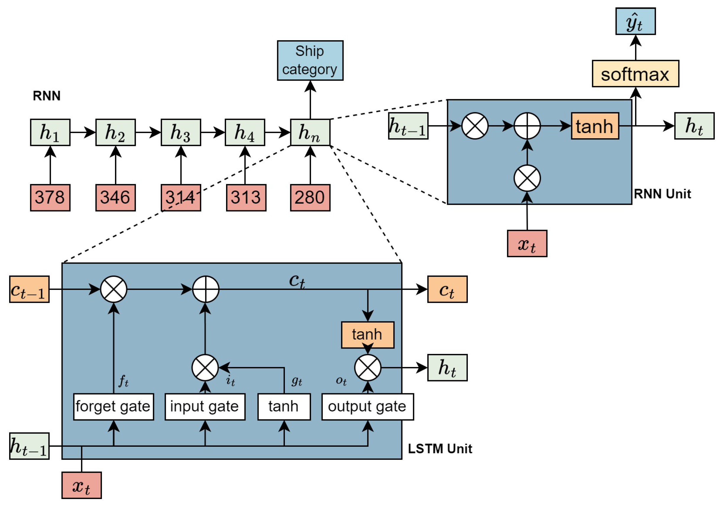
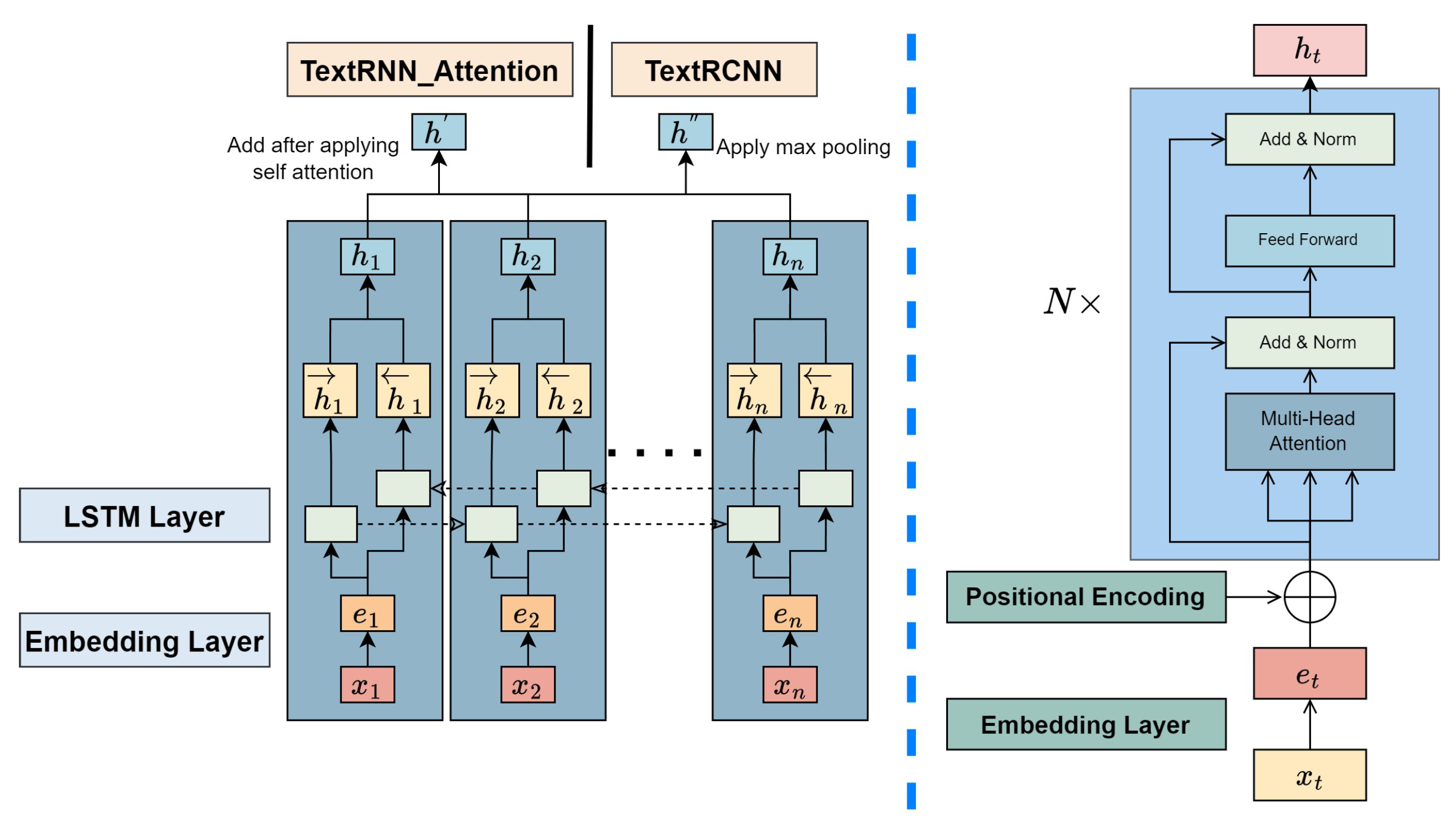
RNNs are crucial in modeling sequential data, especially effective in capturing long-range dependencies via their recurrent computational nature. An RNN language model assimilates past data and considers the relative positional relationship between words. We discuss an RNN model for classifying texts as presented in the top-left diagram of Figure 4.

Here, every input word is symbolized by Word2vec embeddings. These embedded word vectors are input into the RNN unit in sequence, with the output of each RNN unit (dimensionally aligned with the input vectors) fed into the next hidden layer. RNNs are characterized by parameter sharing among different units. The final hidden layer output is utilized for text label prediction.

As depicted in Figure 4, TextRNN is a common RNN module theoretically enabling the unit at time t for information access from all previous time steps. Nonetheless, one major challenge in RNNs is the issue of vanishing gradients during backpropagation. This occurs when continuous multiplication of small derivatives leads to significantly diminished gradients, hindering the RNN’s ability to learn from dependencies over long ranges in sequences. LSTM units were introduced to mitigate this issue. LSTMs maintain an internal memory cell, updating and revealing its contents selectively, thereby better preserving information over longer sequences.

There are various LSTM variants; in our context, we use the nn.LSTM unit from PyTorch. The LSTM unit at time t is defined as a series of vectors with dimensions in ${\mathbb{R}}_d$: the input gate $i_t$, forget gate $f_t$, output gate $o_t$, candidate memory $g_t$, memory cell $c_t$, and hidden state $h_t,i_t,f_t$ and ot are constrained within the range [0,1]. The state transition formulas for LSTM are outlined in the lower diagram of Figure 4.

$$\begin{array}{cc}\hfill i_t& =\sigma (W_{ii}{x}_t+b_{ii}+W_{hi}{h}_{t-1}+b_{hi})\hfill \end{array}$$

(11)

$$\begin{array}{cc}\hfill f_t& =\sigma (W_{if}{x}_t+b_{if}+W_{hf}{h}_{t-1}+b_{hf})\hfill \end{array}$$

(12)

$$\begin{array}{cc}\hfill g_t& =tanh(W_{ig}{x}_t+b_{ig}+W_{hg}{h}_{t-1}+b_{hg})\hfill \end{array}$$

(13)

$$\begin{array}{cc}\hfill o_t& =\sigma (W_{io}{x}_t+b_{io}+W_{ho}{h}_{t-1}+b_{ho})\hfill \end{array}$$

(14)

$$\begin{array}{cc}\hfill c_t& =f_t\odot c_{t-1}+i_t\odot g_t\hfill \end{array}$$

(15)

$$\begin{array}{cc}\hfill h_t& =o_t\odot tanh\left(c_t\right)\hfill \end{array}$$

(16)

where $x_t$ represents the input at time t, $\sigma$ denotes the activation function of sigmoid, which constrains the three gate units’s values to the range [0,1], and ⊙ denotes the Hadamard product.

During text categorization and similar tasks where subsequent time-step information is relevant, a popular choice is the bidirectional LSTM (biLSTM). Unlike standard LSTM, biLSTM processes data in both directions, making it obtain contextual information from past and future time steps. The bidirectional representation $h_t$ is formed by concatenating the forward $\overrightarrow{h_t}$ and backward $\overleftarrow{h_t}$ hidden states. Note that the dimensions of these hidden states in the two directions can differ. biLSTM is widely used for tasks requiring a comprehensive understanding of context.

In the TextRNN+Attention[28] and TextRCNN[29] models, an attention layer is added after the biLSTM layer, as depicted in the left part of Figure 5. The biLSTM layer output of the i-th word is $\overleftrightarrow{h_i}=[\overleftarrow{h_i}\oplus \overrightarrow{h_i}]$. The attention mechanism has shown impressive results in diverse utilizations, like question answering, machine translation, as well as speech recognition.

biLSTM layer output vectors form $H=[h_1,h_2,\cdots ,,h_n]$, where n denotes the sentence length. This symbolization, denoted as r, shows a weighted sum of these output vectors, where $H\in {\mathbb{R}}^{k\times n}$, with k being the word vector dimension. The ultimate sentence representation is marked as $h^{\ast }$. Then, softmax is utilized to estimate the label $\widehat{y}$ for sentence S based on the discrete set of classes Y . To prevent overfitting, dropout and L2 regularization are adopted, incorporating dropout in the embedding, biLSTM, and attention layers.

$$\begin{array}{cc}\hfill M& =tanh\left(H\right)\hfill \end{array}$$

(17)

$$\begin{array}{cc}\hfill \alpha & =softmax\left(w^{T}M\right)\hfill \end{array}$$

(18)

$$\begin{array}{cc}\hfill r& =H{\alpha }^T\hfill \end{array}$$

(19)

$$\begin{array}{cc}\hfill h^{\ast }& =tanhr\hfill \end{array}$$

(20)

TextRCNN seeks to optimize space by concatenating all outputs from the biLSTM layer and using a layer of max pooling to compress them into an individual vector. This vector is then processed through a fully connected layer for dimension reduction, as shown in the left diagram of Figure 5.

2.5.3. Encoder section of the Transformer

The Transformer architecture (Right part of Figure 5), initially proposed for machine translation tasks, represents a significant departure from traditional RNN and CNN structures. In the context of text classification, we utilize exclusively the Encoder part of the Transformer. The Transformer Encoder comprises multiple layers that share the same architecture but possess distinct parameter sets. Inputs to the Transformer are initialized with word vectors trained via Word2vec or with vectors that are randomly initialized.

The Transformer model, setting aside RNNs, processes sequences simultaneously. It incorporates positional embeddings into the initial word embeddings to maintain the sequential order of words. In this system, even and odd positions in the sequence utilize sine and cosine functions, respectively, as demonstrated in Equation 21. The dimensions of these positional embeddings align with the word embeddings, and their combination forms the input to the Encoder.

$$\left\{\begin{array}{c}P{E}_{(}pos,2i)=sin(pos/{10000}^{(2i/d_{model})})\\ P{E}_{(}pos,2i+1)=cos(pos/{10000}^{(2i/d_{model})})\end{array}\right.$$

(21)

Within the Transformer, a mechanism of self-attention is utilized, generating the parameters $Q,K$, and V by multiplying the word embeddings with matrices initialized at random. The detailed mechanism has two features:

• Parallel processing: The computation within self-attention operates independently, allowing for parallel processing which speeds up computations.
• Global information capture: The mechanism computes word relationships independently, treating the distance between words as uniformly one. This feature enables the mechanism to gather global information easily, achieving or exceeding the long-range information capture capabilities of RNNs.

The Transformer Encoder is composed of six layers, each including a multi-head self-attention layer and a fully connected layer. For similarity calculations, the Transformer uses a dot-product approach. However, when the value of K is substantial, the dot-product results can become excessively large, causing the softmax function’s output to tend toward 0 or 1.

To counteract this, a scaling factor is introduced by dk to normalize these dot-product outcomes, as indicated in Equation 22. Furthermore, the mechanism leverages several sets of Q, K, and V matrices, enabling the model to capture diverse information projections. The outcomes from these various heads are combined, as shown in Equation . The Encoder’s feed-forward layer consists of a fully connected layer with ReLU activation. To prevent overfitting, a dropout of 10% is applied following each sub-layer. The fully connected layer includes two linear transformations (Equation ). Additionally, residual connections (x+Sublayer(x)) and layer normalization (LayerNorm(x+Sublayer(x))) are employed, ensuring unique mean and variance for each sample in the LayerNorm.

$$\begin{array}{cc}\hfill \mathrm{Attention}(Q,K,V)& =\mathrm{softmax}\left(\frac{Q{K}^T}{\sqrt{d_k}}\right)V\hfill \\ \hfill \mathrm{MultiHead}(Q,K,V)& =\mathrm{Concat}(hea{d}_1,hea{d}_2,\cdots ,hea{d}_h)W^O\hfill \end{array}$$

(22)

$$\begin{array}{cc}\hfill \mathrm{where}{\mathrm{head}}_{\mathrm{i}}& =\mathrm{Attention}(Q{W}_i^Q,K{W}_i^K,V{W}_i^V)\hfill \end{array}$$

(23)

$$\begin{array}{cc}\hfill \mathrm{FFN}\left(x\right)& =max(0,x{W}_1+b_1)W_2+b_2\hfill \end{array}$$

(24)

2.6. biSAMNet

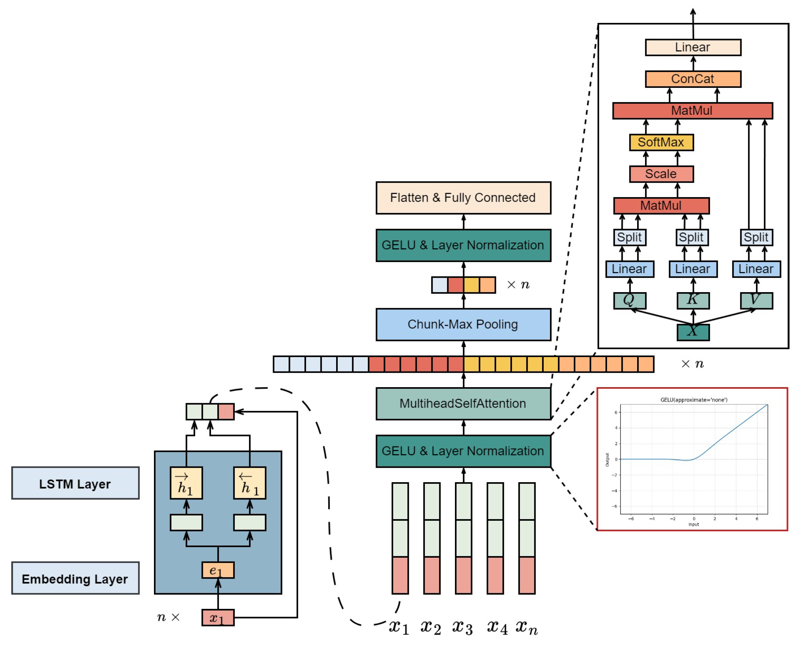
We introduce a new network design, biSAMNet, illustrated in Figure 6. This model combines a bidirectional recurrent framework for capturing contextual information and maintaining word order during text representation learning. It also concatenates the original word embeddings. Notably, biSAMNet employs chunk-max pooling for extracting key text segments. This pooling technique maintains the relative order of multiple local maxima features. While it does not retain precise positional details, it captures a general sense of position due to the initial division into chunks before selecting the maximum values. The network also incorporates the GELU activation function[30], adaptable to various learning rates. GELU, with its curvature at all points and non-monotonic nature, is more effective in approximating complex functions than traditional activation functions like error linear unit (ELU) and RELU.

The architecture of biSAMNet mainly consists of biLSTM, multi-head self-attention layers, and chunk-max pooling layers. For a given text $x_{1:n}$ with a length of n, the network first converts it into word vector representations through an embedding layer. It then processes these vectors using biLSTM to obtain bidirectional outputs at every time interval. At every step, the biLSTM output is combined with the corresponding word vector, creating a semantic vector. Specifically, for word $x_i$,its semantic vector combines the left and right semantic vectors ($c_l\left(x_i\right)$ and $c_r\left(x_i\right)$) with its word embedding vector $e\left(x_i\right)$, as depicted in Equations 25-.

$$\begin{array}{cc}\hfill c_l\left(x_i\right)& =f(W^l{c}_l\left(x_{i-1}\right)+W^{sl}e\left(x_{i-1}\right))\hfill \end{array}$$

(25)

$$\begin{array}{cc}\hfill c_r\left(x_i\right)& =f(W^r{c}_r\left(x_{i+1}\right)+W^{sr}e\left(x_{i+1}\right))\hfill \end{array}$$

(26)

$$\begin{array}{cc}\hfill e^{\ast }\left(x_i\right)& =[c_l\left(x_i\right)\oplus e\left(x_i\right)\oplus c_r\left(x_i\right)]\hfill \end{array}$$

(27)

Next, the concatenated vector is subjected to the GELU activation function (Equation 28), represented in Equation when approximating GELU with the tanh function. This is followed by layer normalization, as shown in Equation , before the data proceeds to the multi-head self-attention layer.

$$\begin{array}{cc}\hfill \mathrm{GELU}& =x\ast \Phi \left(x\right)\hfill \end{array}$$

(28)

$$\begin{array}{cc}\hfill \mathrm{GELU}& =0.5\ast x\ast (1+tanh(\sqrt{\frac{2}{\pi }}\ast (x+0.044715\ast x^3)))\hfill \end{array}$$

(29)

$$\begin{array}{cc}\hfill y& =\frac{x-E\left[x\right]}{\sqrt{Var\left[x\right]}+ϵ}\ast \gamma +\beta \hfill \end{array}$$

(30)

Subsequently, biSAMNet employs a vertical max pooling layer to pinpoint the most significant features in every segment, enabling the network to autonomously determine the key features for text classification. The vertical max pooling layer, detailed in Equation 31, divides the vector into four parts, applies one-dimensional max pooling to each, and generates a $1\times 4$ vector, which vector is flattened and input into a fully connected layer.

$$\mathrm{out}\left(N_i,C_j,k\right)=\underset{m=0,\dots ,{\mathrm{kernel}}_{\mathrm{s}}\mathrm{ize}-1}{max}\mathrm{input}\left(N_i,C_j,\mathrm{stride}\times k+m\right)$$

(31)

3. Results

3.1. Definition of the Problem

This section clarifies essential definitions used throughout the paper. A vessel trajectory, denoted as T, is denoted by a timestamped series of points sourced from AIS devices, that is, $T=t_1,t_2,\cdots ,t_N$, where $t_n=la{t}_n,lo{n}_n,tim{e}_n,n\in [1,2,\cdots ,N]$. Here, n indicates the nth timestamp, and N represents the ship trajectory length. The components $la{t}_n,lo{n}_n$, and $tim{e}_n$ in $t_n$ represent longitude, latitude, and timestamp. Post encoding the grids, $E=e_1,e_2,\cdots ,e_N$, where $e_n\in [1,2,\cdots ,868]$, indicates the numerical representation of the embedded grid point. Applying the word embedding matrix, the input for the model becomes $X=x_1,x_2,\cdots ,x_N$, where $x_i\in {\mathbb{R}}^d$ and d represents the dimension of the embedding. $Y=y_1,y_2,y_3$ denotes the trajectory categories.

Equation 32 defines the cosine similarity between vector A and vector B.

$$sim(A,B)=cos\left(\theta \right)=\frac{A·B}{\left|A\right|\left|B\right|}=\frac{{\sum }_{i=1}^n{A}_i\times B_i}{\sqrt{{\sum }_{i=1}^n{\left(A_i\right)}^2}\times \sqrt{{\sum }_{i=1}^n{\left(B_i\right)}^2}}$$

(32)

3.2. Study Area

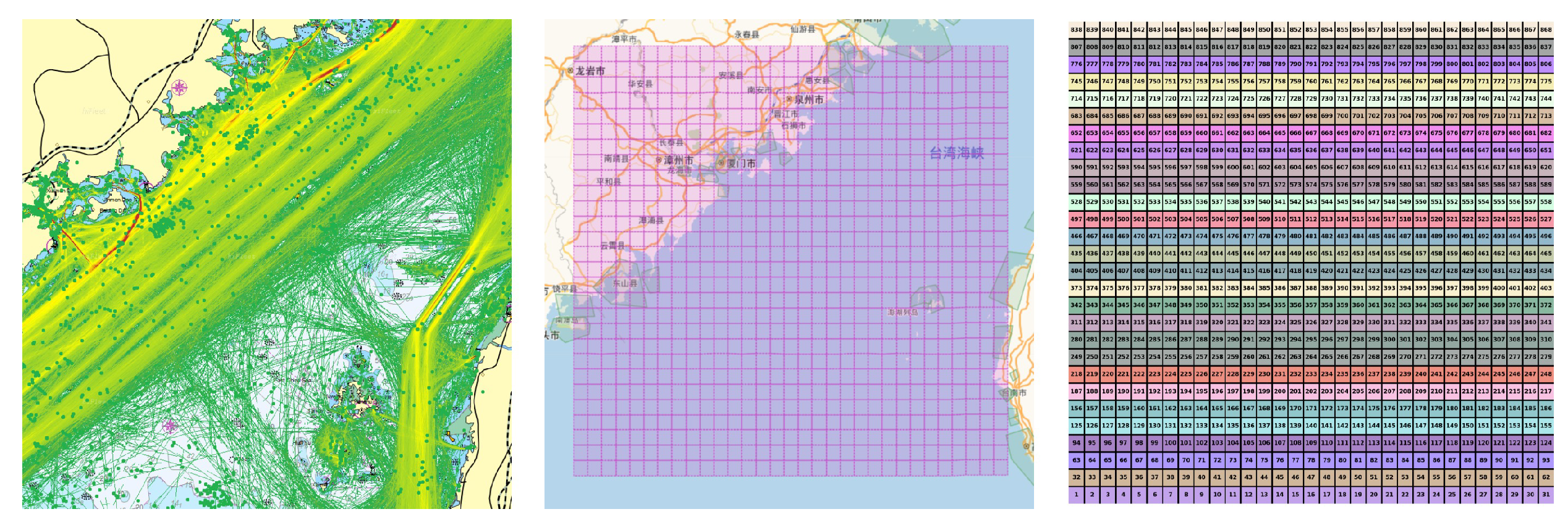
This research takes the Taiwan Strait and its surrounding waters as a case study, a pivotal corridor for China’s coastal shipping and the exclusive direct sea route between Fujian and Taiwan. This region’s western waters, marked by numerous ports, intersecting shipping lanes, and intense commercial activities, form the `Maritime Silk Road’s central part. Neverthelss, the area is known for its challenging meteorological and oceanographic conditions, including hidden reefs and shallow areas, making it a historically risky navigation zone. With growing cross-strait shipping economies and developing ’Maritime Silk Road’ initiative, the navigational complexity in the Taiwan Strait has increased significantly. Recent data indicates that about half of the global container ships traversed this strait last year. The research utilized a maritime heatmap to depict the regional traffic, with a detailed view of the specific area and a chart showing the correspondence of 868 grids, as shown in Figure 7.

3.3. Experimental Data

The experimental dataset, sourced from multiple origins over three years, comprised about 5 billion records. Employing the previously mentioned method, data were processed monthly, resulting in 1,476,109 records. Due to some paths being overly lengthy, a sliding window technique was used, yielding 4 million processed records. Word embedding training utilized the original data, while other experiments used this cleaned dataset. The classification experiment focused on the top 5 most common vessel types in the dataset. Post-comparison with ship profiles, a notable number of vessels remained unclassified, as presented in Table 3.

3.4. Experimental Settings

We divided the dataset into training, validation, and test sets in a 9:0.5:0.5 ratio. For monthly classification, the embedding dimension was set at 100, batch size at 1024, sentence length at 30, and the experiment ran for 100 epochs. Training ceased early if no improvement was observed after 10,000 batches. The Adam optimizer was used for optimization. In TextCNN, four convolutional kernel sizes (2, 3, 4, 5) each with 256 kernels were utilized. Three RNN models used LSTM units with 256 in the hidden layer and 2 layers. The Transformer model featured an embedding dimension of 100, 5 heads, and 6 stacked Encoder layers for feature extraction. Final results were based on test set performance.

As for Word2vec, a window size of 5 was chosen, with the skip-gram model employing a negative sampling training approach.

Dimensionality tests explored embeddings of 1, 20, 50, and 100 dimensions in a 5-class classification experiment using the complete dataset.

In the ablation study, we employed 100-dimensional embeddings and conducted tests with both vectors trained by Word2vec and from random initialization. Using Word2vec embeddings, we additionally examined the effect of freezing the embedding layer during testing.

3.5. Assessment Indicators

This research focused on classifying ship paths, utilizing three key metrics: precision, recall, and F1 score.

$$\begin{array}{c}\hfill \mathrm{precision}=\frac{TP}{TP+FP}\end{array}$$

(33)

$$\begin{array}{c}\hfill \mathrm{recall}=\frac{TP}{TP+FN}\end{array}$$

(34)

$$\begin{array}{c}\hfill {\mathrm{F}}_1\mathrm{score}=2\times \frac{\mathrm{precision}\times \mathrm{recall}}{\mathrm{precision}+\mathrm{recall}}\end{array}$$

(35)

Precision gauges the percentage of accurately classified instances via the model, whereas recall assesses the model’s ability to correctly determine all instances of a particular category. The F1 score, a weighted harmonic mean of precision and recall, is employed to gauge the effectiveness of the categorization model. These metrics were instrumental in assessing the performance of vessel trajectory categorization in our study.

In terms of the cosine similarity comparison, a different approach was adopted. A random sequence, denoted as x, was selected, and the top-k records with the greatest cosine similarity were identified. Records that belonged to the same category as x were considered correct. The top-k ratio, where k represents the number of records with the greatest cosine similarity, was calculated. For example, if x belongs to category A and 3 out of the top 5 most similar records are also in category A, the top-5 ratio is 0.6. Similarly, if 7 out of the top 10 records are correct, the top-10 ratio is 0.7.

$$\mathrm{top}-k=\frac{Truenumberofk}{k}$$

(36)

3.6. Calculation Results of Cosine Similarity

To evaluate the three methods effectively, the study randomly chose 3,000 unique vessel trajectories and computed three metrics: top-5, top-10, and top-20. The vector representation of each trajectory was determined by averaging the embeddings of all grid points along the path.

The outcomes, as illustrated in Table 4, indicate that using Word2vec-trained vectors significantly enhances accuracy. The one-hot method demonstrates lower efficacy across all metrics. There appears to be a notable correlation between Word2vec-trained vectors and ship categories, particularly evident in the Sum-Average method. This could be because the Sum-Average approach effectively leverages the semantic and structural qualities of Word2vec vectors in integrating ship trajectory information. Overall, these results highlight the relative success of different methods in solving ship trajectory classification challenges and underscore the value of Word2vec vectors in understanding and categorizing ship trajectories.

3.7. Path Compression Comparison

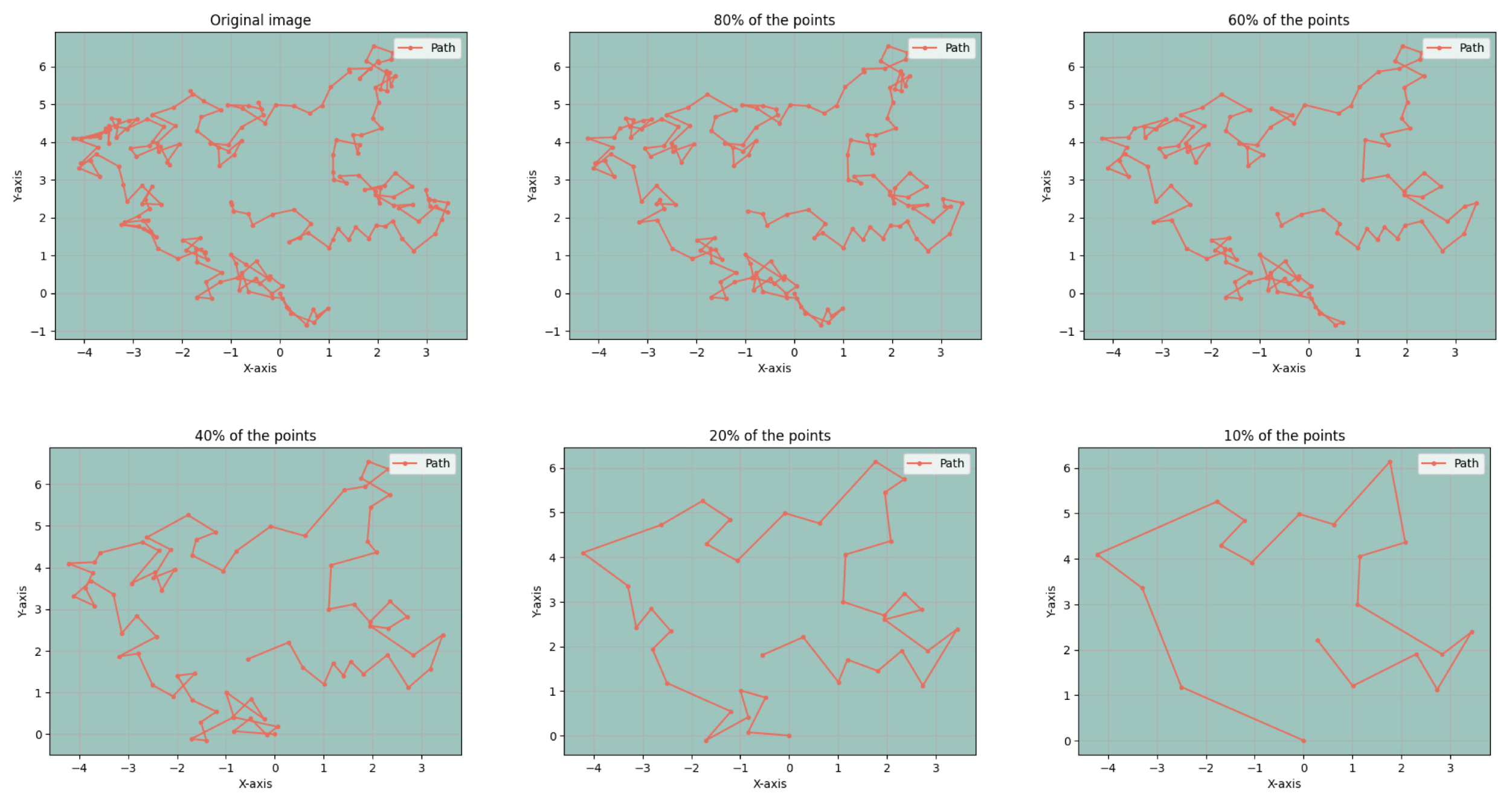
The Visvalingam-Wyatt algorithm has proven highly effective in simplifying path data, successfully reducing the data point count while preserving the path’s essential characteristics. To illustrate this, we selected a random vessel trajectory with 200 data points, with results shown in Figure 8. The trajectory underwent various levels of data reduction, retaining 80%, 60%, 40%, 20%, and 10% of the original points. Despite some data point removal, the fundamental route patterns remained intact. In practical applications, rather than adhering to a fixed data point retention ratio, we set a small triangle area threshold (e.g., 0.001) to dynamically determine the number of points to keep. This method intelligently adjusts the extent of data simplification according to the unique features of each trajectory, efficiently balancing feature preservation and data processing complexity.

3.8. Results of Data Classification for Different Models

In experiments with an embedding dimension of 100, biSAMNet stands out in neural network training. The performance of six models across three metrics is tabulated in Table 5, and a bar chart representation in the left part of Figure 9 further illustrates these findings.

It is noteworthy that, except for Transformer-based models, precision scores consistently exceed recall values in all models, suggesting a tendency towards cautious predictions. Traditional CNN and RNN models surpass the attention-based Transformer models in effectiveness. In particular, the convolutional TextCNN exhibits lower performance metrics compared to RNN-related models. Within the RNN category, adding an attention layer to biLSTM results in improved outcomes. The biSAMNet model, our contribution, showcases superior effectiveness compared to other evaluated models. The underperformance of Transformer models may be attributed to the attention mechanism being more suited to language models. It appears that attention mechanisms may not offer substantial benefits in direct classification predictions using an Encoder or in processing data that is not specifically language-oriented.

3.9. Ablation Analysis and Tests in Various Dimensions

To assess the influence of Word2vec pre-trained models on various deep neural networks, we trained six models using the same dataset, each with an embedding dimension of 50. We experimented with three scenarios: unfreezing the embedding layer, freezing the pre-trained embedding layer, and using randomly initialized embeddings without freezing. The outcomes are summarized in Table 6.

The choice between different embedding layers and model configurations significantly affects the quality of text classification tasks. Generally, utilizing pre-trained layers, whether frozen or trainable, enhances performance for most models. Notably, the TextCNN model performs best with randomly initialized embeddings, suggesting that pre-trained word vectors do not notably benefit this model. For RNN models, the best results consistently come from freezing the pre-trained layer. However, using a trainable pre-trained layer initially shows promise but eventually leads to slight performance decreases. Transformer models display a considerable dependence on pre-trained layers. They struggle to converge with random initialization, even after adjusting various hyperparameters, highlighting the varying sensitivities to initialization strategies across different models.

Given a vocabulary size under 1,000, as opposed to larger sizes in languages like Chinese or English, we also investigated the adequacy of embeddings below 100 dimensions in capturing semantic information. We conducted experiments with embeddings of 5, 10, 20, 50, and 100 dimensions (the last two on the basis of ablation studies), using the weighted F1 score as the evaluation metric.

The results, shown in the right part of Figure 9, reveal some surprising trends. The Transformer model shows high sensitivity to embedding dimensionality, with poor performance at lower dimensions but marked improvements at higher dimensions. The CNN model’s performance similarly improves, stabilizing beyond a 20-dimensional setting. RNN models, in contrast, display excellent performance even at lower dimensions, with minimal enhancement beyond a 5-dimensional setting. The biSAMNet model consistently outperforms others across almost all dimensional scenarios, demonstrating remarkable stability. These findings suggest that RNN models can effectively utilize lower-dimensional embeddings for superior performance.

4. Discussion

Herein, we processed AIS data using grid encoding, transforming the continuous information (latitude and longitude) into discrete grid sequences. The sequences were then approached as natural language, employing a Word2vec word embedding model to generate low-dimensional embeddings for every grid point. Our study introduced the biSAMNet model to classify vessel trajectories converted into grid sequences. This model’s performance was compared with several others, including TextCNN, biLSTM, LSTM with an attention layer, TextRCNN with max pooling, as well as a Transformer Encoder featuring an attention mechanism. The data for these experiments was sourced from the Taiwan Strait and collected over the past three years.

The biSAMNet model demonstrates effective information extraction from grid sequences. Ablation studies were conducted to assess the influence of using Word2vec-trained embeddings in the model’s embedding layer. Results showed that pre-trained embedding layers, especially when frozen, remarkably improve the model’s performance. Additionally, it was noted that the attention layer has a limited effect on improving performance, while CNN models show average performance in this classification task due to their lack of inherent biases.

Future improvements to this research could address several areas. Firstly, the sample imbalance caused by the specific maritime region’s uneven vessel distribution presents a challenge for multi-class classification. We experimented with a one-to-one random grid replacement technique, akin to the approach in a referenced study[31] where each grid corresponded to a Chinese character. However, this method proved less effective, potentially due to the larger number of grids (868) compared to the four protein bases in the reference study, resulting in a maximum F1 score of only 68.3%. Secondly, as more data become available, retraining a language model specifically tailored to this application could be beneficial. Finally, expanding the developed methodology from the Taiwan Strait to global maritime regions presents an exciting avenue for further research and application.