Robust Algorithms for the Analysis of Fast Field Cycling Nuclear Magnetic Resonance Dispersion Curves

Preprint

Article

Robust Algorithms for the Analysis of Fast Field Cycling Nuclear Magnetic Resonance Dispersion Curves

Altmetrics

Downloads

Views

Comments

A peer-reviewed article of this preprint also exists.

This version is not peer-reviewed

Submitted:

16 April 2024

Posted:

16 April 2024

You are already at the latest version

Alerts

Abstract

Fast Field-Cycling (FFC) Nuclear Magnetic Resonance (NMR) relaxometry is a powerful non-destructive magnetic resonance technique that enables, among other things, the investigation of slow molecular dynamics at low magnetic field intensities. FFC-NMR relaxometry measurements provide insight into molecular motion across various timescales within a single experiment. This study focuses on a \textit{model-free} approach, representing the NMRD profile $R_1$ as a linear combination of Lorentzian functions, thereby addressing the challenges of fitting data within an ill-conditioned linear least-squares framework. Tackling this problem, we present a comprehensive review and experimental validation of three regularization approaches to implement the model-free approach to analysing NMRD profiles. These include: (1) \nameUpe, utilizing locally adapted $L_2$ regularization; (2) \nameL, based on $L_1$ penalties; and (3) a hybrid approach combining locally adapted $L_2$ and global $L_1$ penalties. Each method's regularization parameters are determined automatically, according to the Balancing and Uniform Penalty principles. % Our contributions include the implementation and experimental validation of the \nameUpe{} and \nameUp{} algorithms, and the development of a "dispersion analysis" technique to assess the existence range of the estimated parameters. The objective of this work is to delineate the variance in fit quality and correlation time distribution yielded by each algorithm, thus broadening the set of software tools for the analysis of sample structures in FFC-NMR studies. The findings underline the efficacy and applicability of these algorithms in the analysis of NMRD profiles from samples representing different potential scenarios. 1

Keywords:

Subject: Computer Science and Mathematics - Applied Mathematics

1. Introduction

Fast Field-Cycling (FFC) Nuclear Magnetic Resonance (NMR) relaxometry is a powerful non-destructive magnetic resonance technique that allows the exploration of slow molecular dynamics, accessible only at extremely low magnetic field intensities. By varying the strength of the relaxation magnetic fields, FFC enables the assessment of the frequency dispersion of the longitudinal relaxation rate (

R_{1}

) within a sample, consequently producing NMR Dispersion (NMRD) profiles. Consequently, FFC-NMR relaxometry measurements can detect molecular motion across a broad spectrum of timescales within a single experiment.

Under the proper constraints [1], spin relaxation theory characterizes relaxation rates as linear combinations of spectral density functions, which are the Fourier transforms of the time correlation functions. These functions capture the frequencies and their intensities present in the correlation function. Several models exist in the literature (see [2] for a survey) where the longitudinal relaxation rates are related to the parameters representing the physical phenomena occurring in the analyzed sample. Thus, all these approaches depend on the specific sample examined.

An approach that allows greater flexibility is known as model-free [3], where the NMRD profile

R_{1}

is expressed as a linear combination of Lorentzian functions.

The model-free approach leads to a data fit problem consisting of an ill-conditioned linear least-squares problem whose stable solution requires appropriate regularization.

We propose a review of three potential approaches: MF-UPen, which employs locally adapted

L_{2}

regularization; an algorithm based on the

L_{1}

penalty, referred to as MF-L1; and finally, a method called MF-MUPen, that utilizes both locally adapted

L_{2}

and global

L_{1}

penalties. In all these approaches the regularization parameters are computed through automatic procedures founded on the Balancing Principle (BP) [4] and the Uniform Penalty principle [5].

All the algorithms are inspired by two-dimensional time-domain NMR relaxometry techniques. The locally adapted

L_{2}

regularization was originally introduced by Bortolotti et al. in [5], where the regularization parameters are determined by applying the Uniform Penalty principle. The global

L_{1}

regularization has been applied in [6] which addresses the more complex problem of data exhibiting spurious peaks caused by Quadrupolar Relaxation Enhancement. Finally, the coupling of locally adapted

L_{2}

and global

L_{1}

penalties was originally introduced by Bortolotti et al. in [7] for inverting two-dimensional NMR relaxation data and has been adapted to NMRD profiles.

The contributions of this work are the following:

1.: The implementation and experimental testing of the MF-UPen algorithm, featuring a novel rule for automatically computing the threshold parameter $β_{0}$ .
2.: The implementation and experimental testing of the MF-MUPen algorithm.
3.: Development of a "dispersion analysis" procedure, enabling the determination of the existence range for estimated parameters.

Our aim is to illustrate the diversity of results achievable with different algorithms, focusing on fit quality and correlation time distribution. These insights will enrich the suite of software tools available for enhancing sample structure analysis in FFC-NMR studies.

Following this introduction, the mathematical problem and numerical methods are detailed in Section 2 and Section 3, respectively. Section 4 then discusses the results from testing on two sets of NMRD profiles, each representing significant potential scenarios.

2. The Parameter Identification Problem

In the following, we first describe the continuous model for NMRD profiles and then we derive its discretization.

Lo Meo et al. [8] developed a heuristic algorithm to model the NMRD profiles

R_{1} (ω)

based on the model-free approach where the profiles are defined as a combination of two terms:

R_{1} (ω) = R_{0} + R^{H H} (ω)

(1)

where

ω

is the Larmor angular frequency. The first term

R_{0} \geq 0

is an unknown offset keeping into account very fast molecular motions; the second term

R^{H H} (ω)

describes

{}^{1}H - {}^{1}H

relaxation as

R^{H H} (ω) =_{0}^{+ \infty} [\frac{τ}{(1 + {(ω τ)}^{2})} + \frac{4 τ}{(1 + 4 {(ω τ)}^{2})}] f (τ) d τ

(2)

where

τ

represents the correlation time, i.e., the average time required by a molecule to rotate one radiant or to move for a distance as large as its radius of gyration, and f is the distribution to be recovered. Equation (1) identifies a parameter identification problem where the unknown parameters

(f (τ), R_{0})

have to be estimated from NMRD profile values.

By discretizing equation (1), we obtain the following linear system:

y = K f + R_{0},

(3)

where

K \in R^{m \times n}

derives from the discretization of the integral for

R^{H H}

in (2):

K_{i, j} = \frac{τ_{j}}{(1 + {(ω_{i} τ_{j})}^{2})} + \frac{4 τ_{j}}{(1 + 4 {(ω_{i} τ_{j})}^{2})}, i = 1, \dots, m; j = 1, \dots, n .

(4)

with the vector

ω \in R^{m}

representing the m Larmor angular frequency values (

ω = 2 π ν

, with

ν

M H z

) at which the signal

R_{1}

is evaluated. The unknown vector of the correlation times distribution

f \in R^{n}

is obtained by sampling

f (τ)

in n logarithmically equispaced values

τ_{1}, \dots, τ_{n}

. The vector

y \in R^{m}

represents the observations vector, i.e.,

y_{i} = R_{1} (ω_{i})

, with

i = 1, \dots, m

. Generally, for a typical FFC-NMR experiment,

m ≪ n

Defining

x \equiv (f, R_{0}) \in R^{n + 1}

and

K_{e} \equiv [K 1] \in R^{m \times (n + 1)}

we can reformulate (3) in a more compact form:

y = K_{e} x .

(5)

We underline that the model-free analysis provides a fingerprint of the possible motion regimes regardless of their physical-chemical interpretation. In fact, the integral form of the equation (2) unconstrainedly gives only the number of the possible correlation times describing the dynamics of the overall physical system. Instead, the typical approach used in FFC NMR relaxometry requests an ad-hoc mathematical model containing information about the number and meaning of the correlation times that describe a given system [6].

3. The Algorithms

From a mathematical point of view, the estimation of the parameters

f

, and

R_{0}

starting from the experimental observation

y

represents an ill-conditioned linear inverse problem.

In this section, we describe the proposed algorithms based on locally adapted

L_{2}

regularization (MF-UPen),

L_{1}

-based regularization (MF-L1) and multi-penalty consisting of local-

L_{2}

and

L_{1}

penalties (MF-MUPen).

3.0.1. MF-UPen Algorithm

This algorithm, implementing the locally adapted

L_{2}

regularization, solves the following constrained minimization problem:

\begin{matrix} min_{x \geq 0} & \{∥ y - K_{e} {x ∥}_{2}^{2} + \sum_{i = 1}^{n} λ_{i} {(L x)}_{i}^{2}\} \end{matrix}

(6)

with

L = [Δ, 0] \in R^{n \times (n + 1)}

where

Δ

is the discretization of the second derivative operator, according to central finite difference formulas, and

0

is the

n -

components null column vector. Observe that the regularization is imposed only on the parameter

f

since the sum in (6) ranges for indices i from 1 to n. The regularization parameters

λ_{i}

i = 1, \dots, n

are computed according to the following relaxed UPEN principle [5,9]:

λ_{i} = \frac{{∥y - K_{e} x∥}^{2}}{n (β_{0} + β_{p} {max}_{μ \in I_{i}} {(p_{μ})}^{2} + β_{c} {max}_{μ \in I_{i}} {(c_{μ})}^{2})}, i = 1, \dots, n

(7)

where

c = Lx

p = [\nabla, 0] x

and the

I_{i}

are the indices subsets related to the neighborhood of the

i -

th entry, i.e.

I_{i} = \{i - 1, i, i + 1\}

. The

β

’s are positive parameters. The parameter

β_{0}

prevents division by zero and is a compliance floor, which should be small enough to prevent under-smoothing and large enough to avoid over-smoothing. The optimum value of

β

’s could substantially change with the nature of the measured sample.

The parameters

β_{p}, β_{c}

are used to enhance or mitigate the local effects of slope/curvature. A preliminary trial value that often yields satisfactory results is

β_{p} = β_{c} = 1

. The parameter

β_{0}

, however, is more critical; its value should not exceed the threshold defined by

max_{i} \{β_{p} max_{μ \in I_{i}} {(p_{μ})}^{2} + β_{c} max_{μ \in I_{i}} {(c_{μ})}^{2}\},

(8)

while a too-small value, especially in cases where slope

(p)

and curvature

(c)

approach zero, would lead to an extremely ill-conditioned problem, hence causing computational challenges.

Therefore, we propose an automatic rule for determining

β_{0}

based on the estimate of (8) obtained from a tentative solution

\hat{f}

computed by the Truncated Singular Value Decomposition [10] of the matrix

K = U Σ V^{T}

\hat{f} = \sum_{σ_{i} > {Tol}_{σ}} \frac{u_{i}^{T} y}{σ_{i}} v_{i}, {Tol}_{σ} = 10^{- 6} σ_{1},

where

σ_{1} \geq σ_{2} \geq \dots \geq σ_{i} \geq \dots

represent the singular values, and the vectors

u_{i}, v_{i}

represent the i-th columns of U and V, respectively.

By setting:

V_{i} = β_{p} max_{μ \in I_{i}} {({\hat{p}}_{μ})}^{2} + β_{c} max_{μ \in I_{i}} {({\hat{c}}_{μ})}^{2}, i = 1, \dots, n,

where

\hat{c} = Δ \hat{f}

and

\hat{p} = \nabla \hat{f}

, we calculate

β_{0}

as follows:

β_{0} = ρ {∥ V ∥}_{\infty}, 0 < ρ < 1 .

(9)

The advantage of this approach is that it substitutes the parameter

β_{0}

, which can range in

(0, \infty)

, with the parameter

ρ

, which is confined within the interval

(0, 1)

. This substitution ensures that

β_{0}

remains lower than the highest values of V but higher than the lowest ones. This makes determining

β_{0}

more intuitive, particularly when supported by a visual representation of V.

Summarizing, MF-UPen is an iterative scheme where, given an initial guess

λ_{i}^{(0)}

i = 1, \dots, n

, an approximate solution

x^{(k)} \equiv (f^{(k)}, R_{0}^{(k)})

is computed by solving (6) for fixed

λ_{i}^{(k)}

i = 1, \dots, n

, and the regularization parameters values are updated according to (7). The minimization problem (6) is solved by the Newton projection method (NP) [5]. MF-UPen is sketched in Algorithm 1; the iterations are stopped when the following condition is satisfied

\sum_{i = 1}^{n} | λ_{i}^{(k + 1)} - λ_{i}^{(k)} | < Tol \sum_{i = 1}^{n} | λ_{i}^{(k)} |

(10)

where Tol is a fixed tolerance.

Algorithm 1 MF-UPen

1:: Set $k = 0$ , and choose a starting guess $λ_{i}^{(0)}$ , $i = 1, \dots, n$ .
2:: Compute $β_{0}$ according to (9).
3:: repeat
4:: $k = k + 1$
5:: NMRD parameters update. By using the Newton Projection method compute

$x^{(k)} = \arg min_{x} {∥ y - K_{e} x ∥}_{2}^{2} + \sum_{i = 1}^{n} λ_{i}^{(k - 1)} {(L x)}_{i}^{2}$
6:: Regularization parameter update. Set

$\begin{matrix} λ_{i}^{(k)} & = \frac{{∥y - K_{e} x^{(k)}∥}^{2}}{n (β_{0} + β_{p} {max}_{μ \in I_{i}} {(p_{μ}^{(k)})}^{2} + β_{c} {max}_{μ \in I_{i}} {(c_{μ}^{(k)})}^{2})}, i = 1, \dots, n \end{matrix}$
7:: untilconverge condition (10)
8:: return $(f, R_{0}) = x^{(k)}$ ▹ Result $(f, R_{0})$

3.0.2. MF-L1 Algorithm

This algorithm employs an

L_{1}

-norm based penalty, which is preferred for inducing sparsity in

f

. This approach is based on the assumption that the

f (τ)

distribution is a sparse function characterized by only a few non-zero terms.

The problem of parameter identification is reformulated as the following optimization problem:

\begin{matrix} min_{x \geq 0} & \{∥ y - K_{e} {x ∥}_{2}^{2} + α {∥ x ∥}_{1}\} \end{matrix}

(11)

where

α > 0

is the regularization parameter computed according to the Balancing Principle (BP) [4]. Following [6] we rewrite (11) as

\begin{matrix} min_{x} & \{∥ y - K_{e} {x ∥}_{2}^{2} + {α ∥ x ∥}_{1} + η {∥ x ∥}_{2}^{2}\} \\ s . t . & x \geq 0 \end{matrix}

(12)

In this new formulation (12) the last

L_{2}

-based penalty term,

{η ∥ x ∥}_{2}^{2}

, has been introduced only to ensure that

K_{e}^{T} K_{e} + η I

is a definite positive matrix to ensure that (12) is well-posed. It is not a regularization term and a small positive value for

η \approx 10^{- 10}

is fixed.

The MF-L1 algorithm is an iterative procedure where, starting from an initial guess

λ^{(0)}

, at each iteration k, an estimate of the parameters

(f^{(k)}, R_{0}^{(k)})

is computed by solving the parameter estimation problem (12) for fixed

α^{(k)}

, by the truncated Newton interior-point method [11] (see algorithm 2, step (4)). Then a new value

α^{(k + 1)}

is determined by using the BP (see [4] for a deep theoretical discussion). The BP selects the regularization parameter

α

so that the data fidelity and the regularization terms are balanced up to a multiplicative factor

γ

, i.e.,:

{γ α ∥ x ∥}_{1} = ∥ y - K_{e} {x ∥}_{2}^{2} + η {∥ x ∥}_{2}^{2} .

(13)

We fix

γ = 1

, and we obtain the following rule for the parameter selection:

α = \frac{∥ y - K_{e} {x ∥}_{2}^{2} + η {∥ x ∥}_{2}^{2}}{{∥ x ∥}_{1}} .

(14)

The MF-L1 method is summarized in Algorithm 2.

Algorithm 2 MF-L1

1:: Set $k = 0$ , $η = 10^{- 10}$ , and choose a starting guess $α^{(0)}$ .
2:: repeat
3:: $k = k + 1$
4:: NMRD parameters update. By using the truncated Newton interior-point method, compute

$x^{(k)} = \arg min_{x \geq 0} ∥ y - K_{e} {x ∥}_{2}^{2} + α^{(k - 1)} {∥ x ∥}_{1} + η {∥ x ∥}_{2}^{2}$
5:: Regularization parameter update. Set

$α^{(k)} = \frac{∥ y - K_{e} x^{(k)} ∥_{2}^{2} + η {∥ x^{(k)} ∥}_{2}^{2}}{∥ x^{(k)} ∥_{1}}$
6:: until $| α^{(k)} - α^{(k - 1)} | \leq Tol | α^{(k)} |$
7:: return $(f, R_{0}) = x^{(k)}$ ▹ Result $(f, R_{0})$

The Matlab implementation of this algorithm is part of the freeware Matlab tool, ModelFreeFFC, which addresses the more complex issue of data exhibiting spurious peaks caused by Quadrupolar Relaxation Enhancement. The software can be downloaded from https://site.unibo.it/softwaredicam/en/modelfree. For a detailed discussion, please refer to [6].

3.0.3. MF-MUPen Algorithm

This algorithm implements the multi-penalty approach, proposed in [7] for the two-dimensional NMR relaxometry data. MF-MUPen solves the following unconstrained minimization problem:

\begin{matrix} min_{x} & \{∥ y - K_{e} {x ∥}_{2}^{2} + \sum_{i = 1}^{n} λ_{i} {(L x)}_{i}^{2} + α {∥ x ∥}_{1}\} \end{matrix}

(15)

which incorporates both penalty functions from MF-UPen and MF-L1. The regularization parameters are then calculated using (7) for

λ_{i}, i = 1, n

and (14) for

α

Summarizing, MF-MUPen is an iterative scheme where, given an initial guess

λ_{i}^{(0)}

i = 1, \dots, n

, a parameter estimate

(f^{(k)}, R_{0}^{(k)})

is computed by solving (15) for fixed

λ_{i}^{(k)}

i = 1, \dots, n + 1

. Problem (15) is solved by the FISTA method [12] which is one of the most popular methods for minimizing

L_{1}

-penalized least squares functions.

MF-MUPenis stopped when the following condition is satisfied

\sum_{i = 1}^{n} | λ_{i}^{(k + 1)} - λ_{i}^{(k)} | + | α^{(k + 1)} - α^{(k)} | < Tol (\sum_{i = 1}^{n} | λ_{i}^{(k)} | + | α^{(k)} |) .

(16)

MF-MUPen is sketched in Algorithm 3.

Algorithm 3 MF-MUPen

1:: Set $k = 0$ , and choose a starting guess $λ_{i}^{(0)}$ , $i = 1, \dots, n$ , $α^{(0)}$ .
2:: repeat
3:: $k = k + 1$
4:: NMRD parameters update. By using the FISTA method, compute

$x^{(k)} = \arg min_{x} ∥ y - K_{e} {x ∥}_{2}^{2} + \sum_{i = 1}^{n} λ_{i}^{(k - 1)} {(L x)}_{i}^{2} + α^{(k - 1)} {∥ x ∥}_{1}$
5:: Regularization parameter update. Set

$\begin{matrix} λ_{i}^{(k)} & = \frac{{∥y - K_{e} x^{(k)}∥}^{2}}{n (β_{0} + β_{p} {max}_{μ \in I_{i}} {(p_{μ}^{(k)})}^{2} + β_{c} {max}_{μ \in I_{i}} {(c_{μ}^{(k)})}^{2})}, i = 1, \dots, n α^{(k)} & = \frac{{∥y - K_{e} x^{(k)}∥}^{2}}{n ∥ x^{(k)} ∥_{1}} \end{matrix}$
6:: untilconverge condition (16)
7:: return $(f, R_{0}) = x^{(k)}$ ▹ Result $(f, R_{0})$

Algorithms 1,2 and 3 require an initial estimate for the regularization parameters. This can be obtained by computing a rough approximation

\tilde{x}

to the following nonnegatively constrained least squares problem

min_{x \geq 0} {∥ y - K_{e} x ∥}_{2}^{2}

(17)

and then by using the Balancing and Uniform Penalty principles to get the initial guess. More precisely,

α^{(0)} = \frac{∥ y - K_{e} \tilde{x} ∥_{2}^{2} + η {∥ \tilde{x} ∥}_{2}^{2}}{∥ \tilde{x} ∥_{1}}

in Algorithms 2, 3 and

\begin{matrix} λ_{i}^{(0)} & = \frac{{∥y - K_{e} \tilde{x}∥}^{2}}{n (β_{0} + β_{p} {max}_{μ \in I_{i}} {({\tilde{p}}_{μ})}^{2} + β_{c} {max}_{μ \in I_{i}} {({\tilde{c}}_{μ})}^{2})}, i = 1, \dots, n \end{matrix}

in Algorithms 1 and 3.

4. Results and Discussion

In this section, we report and discuss the results obtained by the proposed algorithms on samples of two different materials well representing typical case tests.

In the first part Section 4.1, we present the metrics used to evaluate the results’ quality quantitatively and the experimental setting. In the last part, Section 4.2, we report and discuss the results obtained by the algorithms.

Numerical computations were carried out using Matlab R2022b on a laptop equipped with Apple M1 chip with 16 GB of RAM. Please observe that throughout the section, we refer to the frequencies

ν

instead of the angular frequencies

ω

, i.e.,

ν \equiv ω / (2 π)

4.1. Experimental Setting

The fitted NMRD profiles, computed by algorithms 1, 2 and 3 are compared to the

R_{1}

data by means of the

χ^{2}

value defined as follows:

χ^{2} = \sum_{i = 1}^{m} \frac{{(e_{i} - y_{i})}^{2}}{m - 1}

(18)

where

e

is the estimated data value, i.e.

e = K \tilde{f} + {\tilde{R}}_{0}

with

(\tilde{f}, \tilde{R_{0}})

the computed parameters. We quantitatively compare the computed correlation time distributions

f

given by the three algorithms determining the peak values and the area below

f

in the neighbourhood of such peaks, defining such a value as SpecificWeight. Let us assume that f has

n_{p}

local maxima at the correlation times

τ_{c_{ℓ}}

ℓ = 1, \dots, n_{p}

. Then we define the neighborhood of interest

I_{ℓ}

using the Full Width at Half Maximum parameter, i.e.

I_{ℓ} \equiv [τ_{ℓ}^{l o w}, τ_{ℓ}^{u p}] s . t . f (τ_{ℓ}^{l o w}) = f (τ_{ℓ}^{u p}) = \frac{1}{2} f (τ_{c_{ℓ}}) ℓ = 1, \dots, n_{p} .

We compute the SpecificWeight value for each peak

τ_{c_{ℓ}}

, i.e:

{SpecificWeight}_{ℓ} = \sum_{j = 1}^{n_{ℓ}} τ_{c_{j}} f (τ_{c_{j}}), τ_{c_{j}} \in I_{ℓ},

(19)

where

n_{ℓ}

is the number of correlation times belonging to

I_{ℓ}

ℓ = 1, \dots, n_{p}

The value of the tolerance parameters used in the stopping criteria of all algorithms is

Tol = 10^{- 2}

. Moreover a maximum number of 10 iterations k has been set but never reached. The computational cost is evaluated in terms of execution time.

To test the algorithms’ robustness, we apply them to a set of

s = 500

artificial profiles obtained by adding to

R_{1}

uniformly distributed noise within the experimental error intervals. With these tests, referred as dispersion analysis, we aim to explore the intervals containing the recovered parameter

R_{0}

and how the calculated estimates scatter around the average value. Additionally, we want to examine how the position and value of the peaks change in the recovered correlation times distributions.

4.2. Numerical Results from FFC Measures

We present the results obtained by applying all the algorithms to NMRD profiles obtained from two experimental samples, Manganese and Poplar, respectively. These two samples show how the algorithms’ results can complement each other to improve the overall quality of the information provided. We evaluate the global quality of the examined methods in terms of

χ^{2}

, offset

R_{0}

and computation time.

The

R_{1}

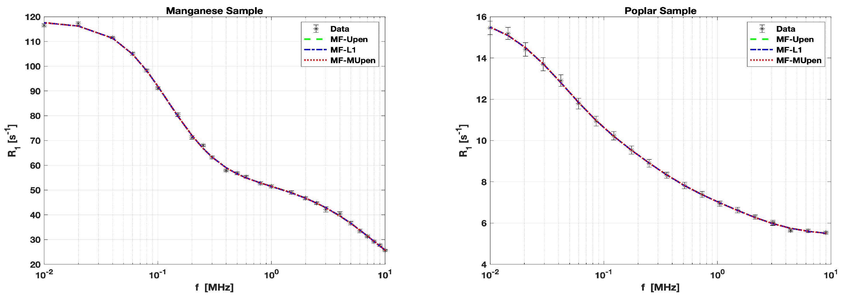
data for the Manganese Sample is measured at 26 frequency values

ν

, ranging from

10^{- 2}

10^{1}

MHz. The error intervals for these measurements vary from

\pm 0.4

\pm 1.1

. These are illustrated by the black error bars in the left panel of Figure 1.

The Table 1 presents the estimated parameter

R_{0}

, the goodness-of-fit measure

χ^{2}

, and the computation time in seconds obtained by the three algorithms. We observe that MF-L1 achieves a moderate

χ^{2}

value and the shortest computation time. In contrast, MF-UPen shows a slightly higher

χ^{2}

and takes longer to compute. Conversely, MF-MUPen achieves the best fit, as evidenced by the lowest

χ^{2}

. This suggests a superior model accuracy, with a modest increase in computation time.

The

R_{1}

data for the Poplar Sample is measured at 21 frequency values

ν

, ranging from

10^{- 2}

10^{1}

MHz. The error intervals for these measurements vary from

\pm 0.06

\pm 0.3

. These are illustrated by the black error bar in the right panel of Figure 1.

The Table 1 outlines the computational results obtained for the Poplar sample by the three algorithms. MF-UPen and MF-L1 both report nearly identical values for

R_{0}

, with minimal

χ^{2}

and very short computation times, indicating efficient and effective performance. However, MF-MUPen, while yielding a similar

R_{0}

to the other two algorithms, shows a higher

χ^{2}

value, suggesting a slightly poorer fit. Additionally, MF-MUPen requires longer computation time.

The outcomes for the Manganese and Poplar samples represent two scenarios, each indicative of the potential variability in sample analysis. This diversity highlights the importance of utilizing multiple methods to fully understand sample characteristics under varying conditions.

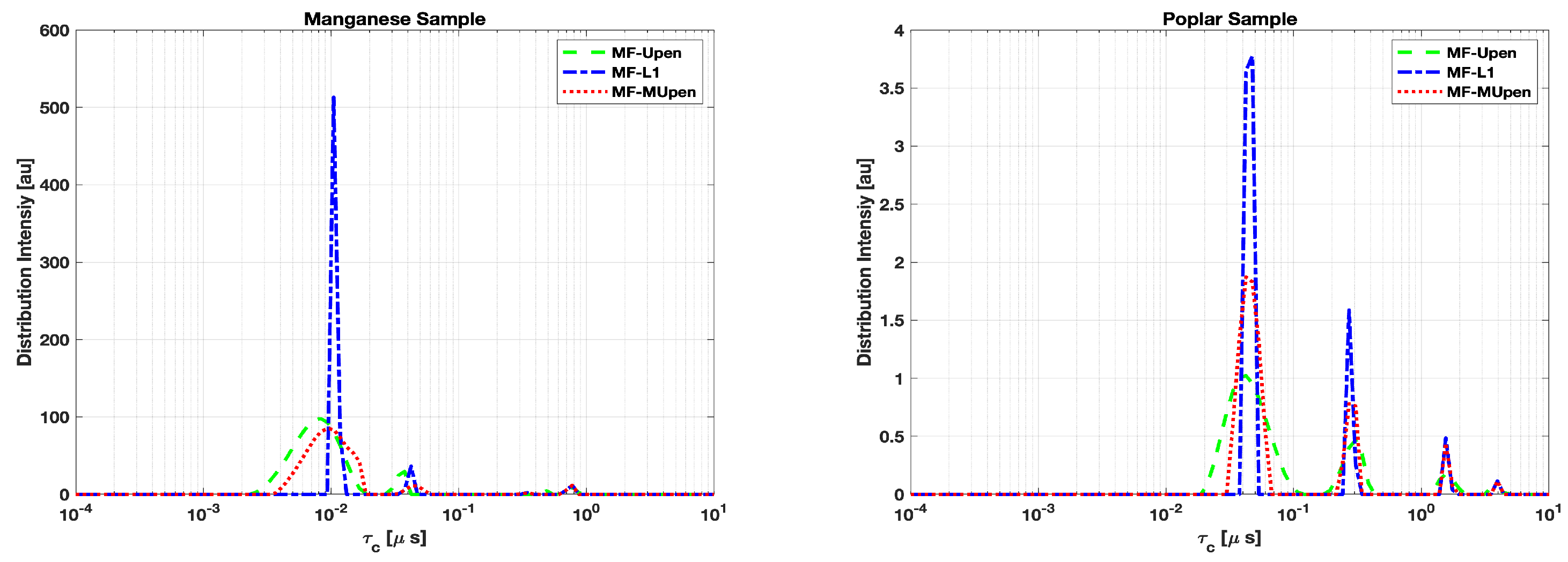
The peak analysis for both the Manganese and Poplar samples across the three methods is performed by plotting the correlation times amplitudes

f

computed by each method in Figure 2 and reporting in the Table 3, Table 4 peaks positions amplitudes, half-width and SpecificWeights for each sample.

In Table 3 we observe a perfect agreement among the three methods in locating the peak at longest correlation time

τ = 7.74 \times 10^{- 1} [μ s]

. While MF-UPen and MF-L1 have a quite good agreement at the intermediate times:

τ_{c} = 3.76 \times 10^{- 2} [μ s]

and

τ_{c} = 4.23 \times 10^{- 2} [μ s]

respectively. The distribution pattern in Figure 2, left panel, shows similarity features between MF-UPen and MF-MUPen and reveals a tendency of MF-L1 to resolve multiple components at the shortest times.

In the case of the Poplar sample, as shown in the right panel of Figure 2 and Table 4, we observe a tighter clustering of peaks across the methods, particularly at the highest amplitude peak around

τ_{c} = 4.23 \times 10^{- 2} [μ s]

. This suggests that all three methods are in agreement concerning the main features of the Poplar sample’s distribution.

4.3. Dispersion Analysis

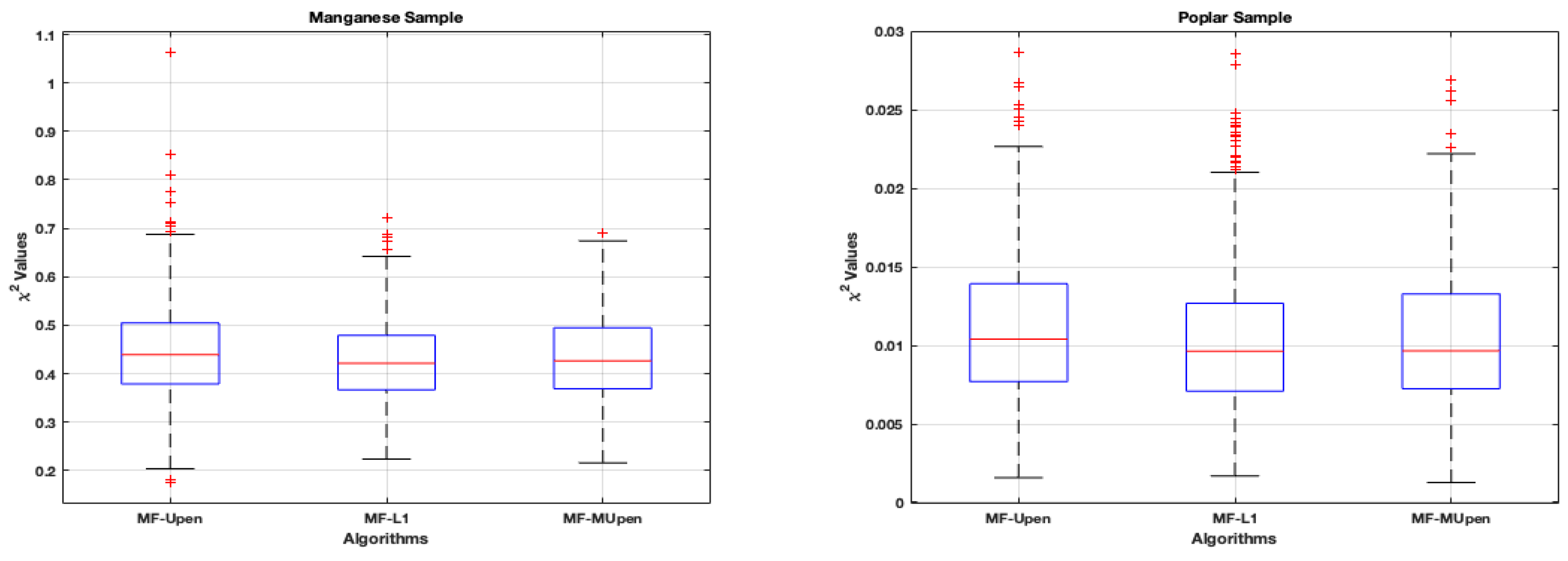
The robustness of the methods is investigated through the dispersion analysis, described in Section 4.1. The boxplots in Figure 3 offer a comparative view of algorithmic performance on the two samples. Each boxplot outlines the algorithms’ interquartile range (IQR) and median of

χ^{2}

values.

We observe uniformity in medians for the Manganese sample, with outliers highlighted by red plus symbols, suggesting occasional significant deviations for MF-UPen. The symmetry of the data is evident from the whiskers’ lengths.

Conversely, the Poplar sample exhibits a tighter IQR for each algorithm, denoting less variability. Despite the close median values indicating consistent algorithmic performance, outliers for MF-L1 reveal notable deviations in some cases.

Table 5 compares the

R_{0}

confidence intervals, mean

R_{0}

, and medians for both Manganese and Poplar samples across the three algorithms.

The confidence intervals and mean

R_{0}

values suggest a wider range of estimates for the Manganese sample, indicating a less uniform agreement among the algorithms. The median values, while closer, still reflect a notable variation between the algorithms, suggesting that the model fit depends on the algorithm applied.

Conversely, the Poplar sample demonstrates remarkable consistency, with both confidence intervals and mean

R_{0}

values being nearly identical across all three algorithms. The median values also closely align, reinforcing the observation of uniform performance. This indicates that for the Poplar sample, the choice of algorithm does not significantly influence the outcome, and all three algorithms provide equivalent information.

Table 5 represents two distinct scenarios that may emerge when these algorithms are applied to samples with varying characteristics. In the case of the Poplar sample, the outcome from all three algorithms is congruent, implying that the algorithms are robust and interchangeable for this type of sample. Conversely, the Manganese sample demonstrates less consistency across the algorithms, suggesting that additional insights from alternative investigative methods are necessary to supplement the analysis.

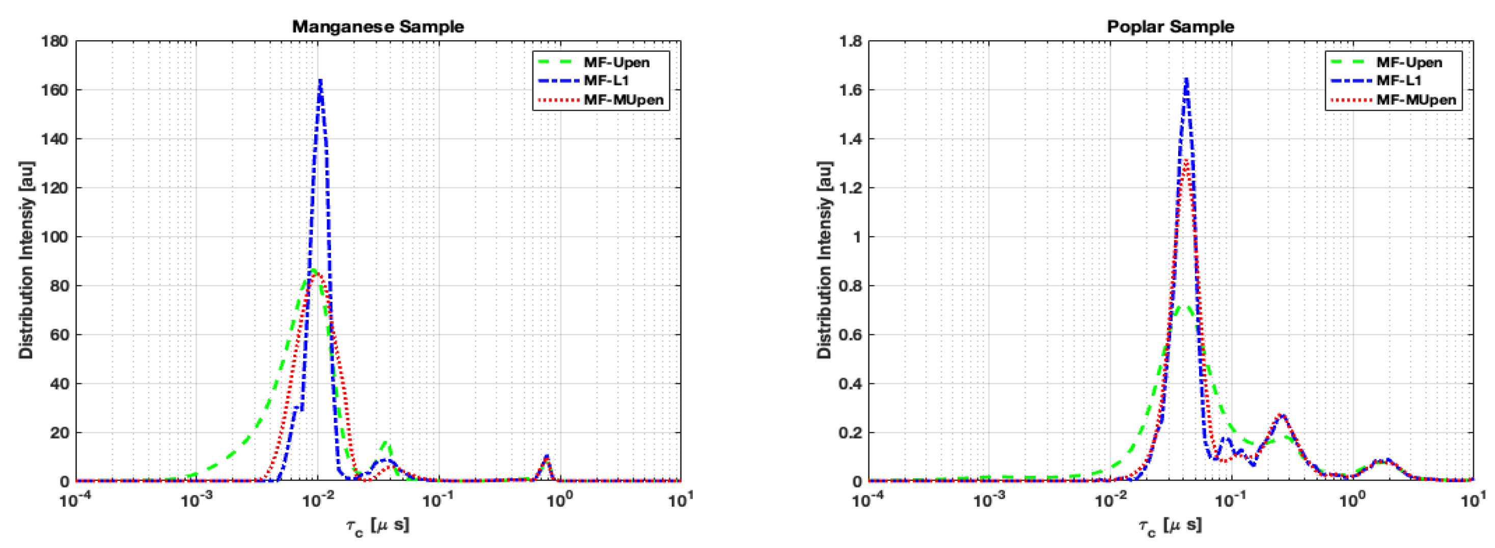
Concerning the distribution intensities, we computed the mean distribution obtained by each method and analyzed the peak positions and amplitudes analogously to Table 1 and Table 4 for the single samples.

From both Table 6 and Table 7 we notice that MF-L1 tends to identify a greater number of peaks compared to the other two methods, suggesting a higher algorithm’s sensitivity.

In the case of the Manganese sample, the data reported in Table 6 show that there is a perfect correspondence in peak position at the longest correlation time

τ_{c} = 7.743 \times 10^{- 1}

among the three algorithms. While the peaks at shortest and intermediate times are split into multiple components.

Concerning the poplar sample (Table 7), we observe that all algorithms show identical peak positioning corresponding to the largest amplitude, reached at the shortest correlation time

τ_{c} = 4.229 \times 10^{- 2} [μ s]

. At longest correlation times, MF-UPen finds a single peak around

τ_{c} = 1.748 \times 10^{0} [μ s]

while MF-L1 and MF-MUPen split the amplitudes in two peaks at

τ_{c} = 1.556 \times 10^{0}, 1.963 \times 10^{0} [μ s]

and

τ_{c} = 1.556 \times 10^{0}, 2.205 \times 10^{0} [μ s]

respectively.

However, despite the differences in the number of peaks identified, Figure 4 shows that all three algorithms exhibit a fundamental robustness in the localization of the positions of the highest peaks.

From Table 5, we observe that MF-MUPen has the smallest confidence intervals in both samples and Figure 3 shows that the number of outliers in MF-MUPen is smaller than in the other methods. This, together with Figure 4, suggests a higher robustness of MF-MUPen compared to the other methods.

5. Conclusion

This study reviews three algorithms designed for the analysis of NMRD profiles from experimental data, showing their efficacy in two different datasets representative of possible applicative scenarios. The comparative analysis of the three algorithms, while revealing a general consistency in identifying the primary peak positions, shows that MF-MUPen exhibits higher robustness in the presence of data noise.

In conclusion, the proposed algorithms have the potential to significantly improve the quality of NMRD profile analysis and enrich the toolkit available to researchers for investigating the molecular dynamics of various samples.

References

Kimmich, R.; Anoardo, E. Field-cycling NMR relaxometry. Progress in Nuclear Magnetic Resonance Spectroscopy 2004, 44, 257–320. [Google Scholar] [CrossRef]
Bortolotti, V.; Brizi, L.; Landi, G.; Testa, C.; Zama, F. Introduction to FFC NMR Theory and Models for Complex and Confined Fluids 2024.
Halle, B.; Jóhannesson, H.; Venu, K. Model-Free Analysis of Stretched Relaxation Dispersions. Journal of Magnetic Resonance 1998, 135, 1–13. [Google Scholar] [CrossRef] [PubMed]
Ito, K.; Jin, B.; Takeuchi, T. A Regularization Parameter for Nonsmooth Tikhonov Regularization. SIAM Journal on Scientific Computing 2011, 33, 1415–1438. [Google Scholar] [CrossRef]
Bortolotti, V.; Brown, R.J.S.; Fantazzini, P.; Landi, G.; Zama, F. Uniform Penalty Inversion of two-dimensional NMR relaxation data. Inverse Problems 2016, 33, 19. [Google Scholar] [CrossRef]
Landi, G.; Spinelli, G.; Zama, F.; Martino, D.C.; Conte, P.; Lo Meo, P.; Bortolotti, V. An automatic L1-based regularization method for the analysis of FFC dispersion profiles with quadrupolar peaks. Applied Mathematics and Computation 2023, 444, 127809. [Google Scholar] [CrossRef]
Bortolotti, V.; Landi, G.; Zama, F. 2DNMR data inversion using locally adapted multi-penalty regularization. Computational Geosciences 2020, 25, 1215–1228. [Google Scholar] [CrossRef]
Lo Meo, P.; Terranova, S.; Di Vincenzo, A.; Chillura Martino, D.; Conte, P. Heuristic Algorithm for the Analysis of Fast Field Cycling (FFC) NMR Dispersion Curves. Analytical Chemistry 2021. [Google Scholar] [CrossRef] [PubMed]
Bortolotti, V.; Brown, R.; Fantazzini, P.; Landi, G.; Zama, F. I2DUPEN: Improved 2DUPEN algorithm for inversion of two-dimensional NMR data. Microporous and Mesoporous Materials 2018, 269, 195–198. [Google Scholar] [CrossRef]
Hansen, P.C. Truncated singular value decomposition solutions to discrete ill-posed problems with ill-determined numerical rank. SIAM Journal on Scientific and Statistical Computing 1990, 11, 503–518. [Google Scholar] [CrossRef]
Kim, S.J.; Koh, K.; Lustig, M.; Boyd, S.; Gorinevsky, D. An Interior-Point Method for Large-Scale ℓ₁-Regularized Least Squares. IEEE Journal of Selected Topics in Signal Processing 2007, 1, 606–617. [Google Scholar] [CrossRef]
Beck, A.; Teboulle, M. A fast iterative shrinkage-thresholding algorithm for linear inverse problems. SIAM journal on imaging sciences 2009, 2, 183–202. [Google Scholar] [CrossRef]

Figure 1. Comparison of

R_{1}

relaxation rates for the Manganese and Poplar samples. The plots show the comparative analysis between the actual data and the results from the MF-UPen, MF-L1, and MF-MUPen algorithms.

Figure 1. Comparison of

R_{1}

relaxation rates for the Manganese and Poplar samples. The plots show the comparative analysis between the actual data and the results from the MF-UPen, MF-L1, and MF-MUPen algorithms.

Figure 2. Distribution intensity as a function of

τ_{c}

for the Manganese and Poplar samples. The plots show the results from the MF-UPen, MF-L1, and MF-MUPen algorithms.

Figure 2. Distribution intensity as a function of

τ_{c}

for the Manganese and Poplar samples. The plots show the results from the MF-UPen, MF-L1, and MF-MUPen algorithms.

Figure 3. Boxplot of the

χ^{2}

values for the Manganese and Poplar samples, comparing the results of the different algorithms on 500 data realizations.

Figure 3. Boxplot of the

χ^{2}

values for the Manganese and Poplar samples, comparing the results of the different algorithms on 500 data realizations.

Figure 4. Mean distribution amplitude over 500 data realizations for Manganese and Poplar samples.

Table 1. Manganese Sample. Computational results of the proposed methods.

Algorithm	$R_{0}$	$χ^{2}$	Computation Time [s]
MF-UPen	$6.64 \times 10^{0}$	$6.23 \times 10^{- 1}$	$9.86 \times 10^{- 1}$
MF-L1	$1.19 \times 10^{1}$	$5.55 \times 10^{- 1}$	$1.35 \times 10^{- 1}$
MF-MUPen	$9.98 \times 10^{0}$	$4.10 \times 10^{- 1}$	$1.24 \times 10^{0}$

Table 2. Poplar Sample. Computational results of the proposed methods.

Algorithm	$R_{0}$	$χ^{2}$	Computation Time [s]
MF-UPen	$5.40 \times 10^{0}$	$7.94 \times 10^{- 3}$	$7.41 \times 10^{- 2}$
MF-L1	$5.41 \times 10^{0}$	$8.84 \times 10^{- 3}$	$6.65 \times 10^{- 2}$
MF-MUPen	$5.41 \times 10^{0}$	$2.19 \times 10^{- 2}$	$3.76 \times 10^{- 1}$

Table 3. Manganese Sample Analysis. Position (

τ_{c}

) and amplitude

f (τ_{c})

of the distribution peaks sorted by

f (τ_{c})

Table 3. Manganese Sample Analysis. Position (

τ_{c}

) and amplitude

f (τ_{c})

of the distribution peaks sorted by

f (τ_{c})

Algorithm	$τ_{c} [μ s]$	$f (τ_{c})$	Half-width	SpecificWeight
MF-UPen	$8.30 \times 10^{- 3}$	$9.78 \times 10^{1}$	$8.19 \times 10^{- 3}$	$6.94 \times 10^{0}$
	$3.76 \times 10^{- 2}$	$2.95 \times 10^{1}$	$8.47 \times 10^{- 3}$	$2.13 \times 10^{0}$
	$7.74 \times 10^{- 1}$	$9.61 \times 10^{0}$	$1.18 \times 10^{- 1}$	$1.09 \times 10^{1}$
	$4.86 \times 10^{- 1}$	$4.63 \times 10^{0}$	$5.67 \times 10^{- 2}$	$2.25 \times 10^{0}$
	$3.43 \times 10^{- 1}$	$4.85 \times 10^{- 2}$	$4.98 \times 10^{- 2}$	$2.17 \times 10^{- 2}$
MF-L1	$1.05 \times 10^{- 2}$	$5.13 \times 10^{2}$	$1.34 \times 10^{- 3}$	$6.30 \times 10^{0}$
	$4.23 \times 10^{- 2}$	$3.63 \times 10^{1}$	$5.36 \times 10^{- 3}$	$1.75 \times 10^{0}$
	$7.74 \times 10^{- 1}$	$1.16 \times 10^{1}$	$1.21 \times 10^{- 1}$	$1.24 \times 10^{1}$
	$3.43 \times 10^{- 1}$	$2.28 \times 10^{0}$	$4.00 \times 10^{- 2}$	$7.84 \times 10^{- 1}$
	$1.63 \times 10^{- 3}$	$3.79 \times 10^{- 3}$	$7.04 \times 10^{- 4}$	$5.17 \times 10^{- 5}$
MF-MUPen	$9.33 \times 10^{- 3}$	$8.49 \times 10^{1}$	$1.09 \times 10^{- 2}$	$6.98 \times 10^{0}$
	$4.75 \times 10^{- 2}$	$1.09 \times 10^{1}$	$1.55 \times 10^{- 2}$	$1.47 \times 10^{0}$
	$7.74 \times 10^{- 1}$	$1.15 \times 10^{1}$	$1.23 \times 10^{- 1}$	$1.24 \times 10^{1}$
	$3.43 \times 10^{- 1}$	$1.49 \times 10^{0}$	$5.24 \times 10^{- 2}$	$7.56 \times 10^{- 1}$

Table 4. Poplar Sample Analysis. Position (

τ_{c}

) and amplitude

f (τ_{c})

of the distribution peaks sorted by

f (τ_{c})

Table 4. Poplar Sample Analysis. Position (

τ_{c}

) and amplitude

f (τ_{c})

of the distribution peaks sorted by

f (τ_{c})

Algorithm	$τ_{c} [μ s]$	$f (τ_{c})$	Half-width	SpecificWeight
MF-UPen	$4.23 \times 10^{- 2}$	$1.02 \times 10^{0}$	$3.92 \times 10^{- 2}$	$3.54 \times 10^{- 1}$
	$3.05 \times 10^{- 1}$	$4.65 \times 10^{- 1}$	$1.25 \times 10^{- 1}$	$5.00 \times 10^{- 1}$
	$1.56 \times 10^{- 1}$	$1.75 \times 10^{- 1}$	$5.38 \times 10^{- 1}$	$8.05 \times 10^{- 1}$
	$3.51 \times 10^{- 1}$	$5.53 \times 10^{- 2}$	$9.32 \times 10^{- 1}$	$4.53 \times 10^{- 1}$
MF-L1	$4.75 \times 10^{- 2}$	$3.77 \times 10^{0}$	$1.04 \times 10^{- 2}$	$3.34 \times 10^{- 1}$
	$2.72 \times 10^{- 1}$	$1.59 \times 10^{0}$	$3.50 \times 10^{- 2}$	$5.11 \times 10^{- 1}$
	$1.56 \times 10^{- 1}$	$4.85 \times 10^{- 1}$	$1.89 \times 10^{- 1}$	$8.20 \times 10^{- 1}$
	$3.94 \times 10^{- 1}$	$1.15 \times 10^{- 1}$	$4.60 \times 10^{- 1}$	$4.55 \times 10^{- 1}$
MF-MUPen	$4.23 \times 10^{- 2}$	$1.87 \times 10^{0}$	$2.13 \times 10^{- 2}$	$3.40 \times 10^{- 1}$
	$2.72 \times 10^{- 1}$	$7.80 \times 10^{- 1}$	$7.49 \times 10^{- 2}$	$5.11 \times 10^{- 1}$
	$1.56 \times 10^{- 1}$	$4.41 \times 10^{- 1}$	$2.02 \times 10^{- 1}$	$8.19 \times 10^{- 1}$
	$3.94 \times 10^{- 1}$	$1.14 \times 10^{- 1}$	$4.60 \times 10^{- 1}$	$4.50 \times 10^{- 1}$

Table 5. Comparison of R0 Confidence Intervals, Mean R0, and Median for Manganese and Poplar samples.

Sample	Algorithm	R0 Confidence Interval	R0 Mean	Median
Manganese	MF-UPen	[5.240, 9.253]	$7.25 \times 10^{0}$	$8.26 \times 10^{0}$
	MF-L1	[9.251, 12.12]	$1.07 \times 10^{1}$	$1.12 \times 10^{1}$
	MF-MUPen	[9.652, 11.38]	$1.05 \times 10^{1}$	$1.05 \times 10^{1}$
Poplar	MF-UPen	[5.363, 5.406]	$5.39 \times 10^{0}$	$5.39 \times 10^{0}$
	MF-L1	[5.370, 5.413]	$5.39 \times 10^{0}$	$5.39 \times 10^{0}$
	MF-MUPen	[5.370, 5.416]	$5.39 \times 10^{0}$	$5.39 \times 10^{0}$

Table 6. Manganese Sample. Analysis of mean distribution over 500 realizations. Position (

τ_{c}

) and amplitude

f (τ_{c})

of the distribution peaks sorted by

f (τ_{c})

Table 6. Manganese Sample. Analysis of mean distribution over 500 realizations. Position (

τ_{c}

) and amplitude

f (τ_{c})

of the distribution peaks sorted by

f (τ_{c})

Algorithm	$τ_{c} [μ s]$	$f (τ_{c})$	Half-width	SpecificWeight
MF-UPen	$9.326 \times 10^{- 3}$	$8.640 \times 10^{1}$	$8.889 \times 10^{- 3}$	$6.949 \times 10^{0}$
	$3.765 \times 10^{- 2}$	$1.727 \times 10^{1}$	$9.075 \times 10^{- 3}$	$1.617 \times 10^{0}$
	$7.743 \times 10^{- 1}$	$9.004 \times 10^{0}$	$1.385 \times 10^{- 1}$	$1.168 \times 10^{1}$
	$5.462 \times 10^{- 1}$	$9.534 \times 10^{- 1}$	$1.139 \times 10^{- 1}$	$4.464 \times 10^{0}$
	$5.995 \times 10^{- 2}$	$7.407 \times 10^{- 1}$	$7.643 \times 10^{- 3}$	$1.208 \times 10^{- 1}$
MF-L1	$1.048 \times 10^{- 2}$	$1.642 \times 10^{2}$	$4.173 \times 10^{- 3}$	$6.216 \times 10^{0}$
	$6.579 \times 10^{- 3}$	$3.024 \times 10^{1}$	$4.493 \times 10^{- 4}$	$5.120 \times 10^{- 1}$
	$7.743 \times 10^{- 1}$	$1.061 \times 10^{1}$	$1.264 \times 10^{- 1}$	$1.215 \times 10^{1}$
	$3.765 \times 10^{- 2}$	$8.763 \times 10^{0}$	$1.897 \times 10^{- 2}$	$1.702 \times 10^{0}$
	$3.854 \times 10^{- 1}$	$5.470 \times 10^{- 1}$	$7.072 \times 10^{- 2}$	$5.642 \times 10^{- 1}$
	$4.863 \times 10^{- 1}$	$3.761 \times 10^{- 1}$	$3.575 \times 10^{- 2}$	$4.885 \times 10^{- 1}$
	$2.420 \times 10^{- 1}$	$1.233 \times 10^{- 1}$	$1.700 \times 10^{- 2}$	$7.589 \times 10^{- 2}$
MF-MUPen	$1.048 \times 10^{- 2}$	$8.461 \times 10^{1}$	$9.725 \times 10^{- 3}$	$6.954 \times 10^{0}$
	$7.743 \times 10^{- 1}$	$9.675 \times 10^{0}$	$1.466 \times 10^{- 1}$	$1.219 \times 10^{1}$
	$4.229 \times 10^{- 2}$	$5.630 \times 10^{0}$	$2.526 \times 10^{- 2}$	$2.163 \times 10^{0}$
	$4.863 \times 10^{- 1}$	$4.064 \times 10^{- 1}$	$1.402 \times 10^{- 1}$	$9.117 \times 10^{- 1}$

Table 7. Poplar Sample. Analysis of mean distribution over 500 realizations. Position (

τ_{c}

) and amplitude

f (τ_{c})

of the distribution peaks sorted by

f (τ_{c})

Table 7. Poplar Sample. Analysis of mean distribution over 500 realizations. Position (

τ_{c}

) and amplitude

f (τ_{c})

of the distribution peaks sorted by

f (τ_{c})

Algorithm	$τ_{c} [μ s]$	$f (τ_{c})$	Half-width	SpecificWeight
MF-UPen	$4.229 \times 10^{- 2}$	$7.234 \times 10^{- 1}$	$5.094 \times 10^{- 2}$	$3.369 \times 10^{- 1}$
	$2.719 \times 10^{- 1}$	$1.830 \times 10^{- 1}$	$8.540 \times 10^{- 2}$	$2.547 \times 10^{- 1}$
	$1.748 \times 10^{0}$	$7.503 \times 10^{- 2}$	$1.211 \times 10^{0}$	$1.091 \times 10^{0}$
MF-L1	$4.229 \times 10^{- 2}$	$1.652 \times 10^{0}$	$1.794 \times 10^{- 2}$	$2.811 \times 10^{- 1}$
	$2.719 \times 10^{- 1}$	$2.662 \times 10^{- 1}$	$1.465 \times 10^{- 1}$	$4.595 \times 10^{- 1}$
	$8.498 \times 10^{- 2}$	$1.744 \times 10^{- 1}$	$2.187 \times 10^{- 2}$	$6.473 \times 10^{- 2}$
	$1.204 \times 10^{- 1}$	$1.287 \times 10^{- 1}$	$1.081 \times 10^{- 2}$	$3.840 \times 10^{- 2}$
	$1.963 \times 10^{0}$	$8.927 \times 10^{- 2}$	$1.045 \times 10^{0}$	$1.007 \times 10^{0}$
	$1.556 \times 10^{0}$	$8.810 \times 10^{- 2}$	$1.176 \times 10^{- 1}$	$3.459 \times 10^{- 1}$
	$6.136 \times 10^{- 1}$	$2.873 \times 10^{- 2}$	$7.136 \times 10^{- 2}$	$4.805 \times 10^{- 2}$
	$7.925 \times 10^{0}$	$1.298 \times 10^{- 3}$	$5.589 \times 10^{- 1}$	$2.304 \times 10^{- 2}$
MF-MUPen	$4.229 \times 10^{- 2}$	$1.312 \times 10^{0}$	$2.518 \times 10^{- 2}$	$3.009 \times 10^{- 1}$
	$2.420 \times 10^{- 1}$	$2.697 \times 10^{- 1}$	$1.420 \times 10^{- 1}$	$4.568 \times 10^{- 1}$
	$1.072 \times 10^{- 1}$	$1.047 \times 10^{- 1}$	$2.110 \times 10^{- 2}$	$5.096 \times 10^{- 2}$
	$1.556 \times 10^{0}$	$7.936 \times 10^{- 2}$	$1.204 \times 10^{0}$	$1.180 \times 10^{0}$
	$2.205 \times 10^{0}$	$7.194 \times 10^{- 2}$	$1.217 \times 10^{- 1}$	$2.996 \times 10^{- 1}$
	$6.893 \times 10^{- 1}$	$2.774 \times 10^{- 2}$	$1.504 \times 10^{- 1}$	$8.125 \times 10^{- 2}$
	$4.431 \times 10^{0}$	$7.331 \times 10^{- 3}$	$2.851 \times 10^{- 1}$	$7.834 \times 10^{- 2}$

Disclaimer/Publisher’s Note: The statements, opinions and data contained in all publications are solely those of the individual author(s) and contributor(s) and not of MDPI and/or the editor(s). MDPI and/or the editor(s) disclaim responsibility for any injury to people or property resulting from any ideas, methods, instructions or products referred to in the content.

© 2024 by the authors. Licensee MDPI, Basel, Switzerland. This article is an open access article distributed under the terms and conditions of the Creative Commons Attribution (CC BY) license (https://creativecommons.org/licenses/by/4.0/).

Copyright: This open access article is published under a Creative Commons CC BY 4.0 license, which permit the free download, distribution, and reuse, provided that the author and preprint are cited in any reuse.

MDPI Initiatives

Important Links

Choose an area of interest and we will send you notifications of new preprints at your preferred frequency.

Disclaimer

Robust Algorithms for the Analysis of Fast Field Cycling Nuclear Magnetic Resonance Dispersion Curves

Abstract

1. Introduction

2. The Parameter Identification Problem

3. The Algorithms

3.0.1. MF-UPen Algorithm

3.0.2. MF-L1 Algorithm

3.0.3. MF-MUPen Algorithm

4. Results and Discussion

4.1. Experimental Setting

4.2. Numerical Results from FFC Measures

4.3. Dispersion Analysis

5. Conclusion

References

MDPI Initiatives

Important Links

Subscribe