Submitted:
15 April 2024
Posted:
18 April 2024
You are already at the latest version
Abstract
Keywords:
1. Introduction
2. Background
2.1. Trust in AI for decision-making
2.2. Quantum Probability Theory
2.3. Modeling Human-AI Decision-Making with Quantum Probability
2.4. Quantum Open Systems Approach
2.5. Trust and Ontic Uncertainty
3. Methods
3.1. Participants
3.2. Overall Design
3.3. Experimental Procedure
4. Results
4.1. Modeling Delegation Strength with Quantum Open Systems to the Study Data
4.2. Comparison of Markov and Quantum Models
5. Quantum Open Systems
5.1. Quantum Open Systems Equation Components and Explanations

5.2. Exploratory Analysis
6. Discussion
6.1. Limitations
6.2. Future Research
7. Summary
Funding
Institutional Review Board Statement
References
- A. Fuchs, A. Passarella, and M. Conti, “Modeling, replicating, and predicting human behavior: a survey,” ACM Trans. Auton. Adapt. Syst., Jan. 2023. [CrossRef]
- L. Waardenburg, M. Huysman, and A. V. Sergeeva, “In the land of the blind, the one-eyed man is king: knowledge brokerage in the age of learning algorithms,” Organ. Sci., vol. 33, no. 1, pp. 59–82, Jan. 2022. [CrossRef]
- P. J. Denning and J. Arquilla, “The context problem in artificial intelligence,” Commun. ACM, vol. 65, no. 12, pp. 18–21, Nov. 2022. [CrossRef]
- D. Blair, J. O. Chapa, S. Cuomo, and J. Hurst, “Humans and hardware: an exploration of blended tactical workflows using john boyd’s ooda loop,” in The Conduct of War in the 21st Century, Routledge, 2021.
- M. Wrzosek, “Challenges of contemporary command and future military operations | Scienti,” Sci. J. Mil. Univ. Land Forces, vol. 54, no. 1, pp. 35–51, 2022.
- A. Bisantz, J. Llinas, Y. Seong, R. Finger, and J.-Y. Jian, “Empirical investigations of trust-related systems vulnerabilities in aided, adversarial decision making,” State Univ of New York at Buffalo center of multisource information fusion, Mar. 2000. Accessed: Apr. 30, 2022. [Online]. Available: https://apps.dtic.mil/sti/citations/ADA389378.
- D. R. Hestad, “A discretionary-mandatory model as applied to network centric warfare and information operations,” NAVAL POSTGRADUATE SCHOOL MONTEREY CA, Mar. 2001. Accessed: Apr. 30, 2022. [Online]. Available: https://apps.dtic.mil/sti/citations/ADA387764.
- S. Marsh and M. R. Dibben, “The role of trust in information science and technology,” Annu. Rev. Inf. Sci. Technol., vol. 37, no. 1, pp. 465–498, 2003. [CrossRef]
- D. Kahneman, Thinking, Fast and Slow, 1st edition. New York: Farrar, Straus and Giroux, 2013.
- J. R. Busemeyer and P. D. Bruza, Quantum models of cognition and decision, Reissue edition. Cambridge: Cambridge University Press, 2014.
- P. V. Thayyib et al., “State-of-the-Art of Artificial Intelligence and Big Data Analytics Reviews in Five Different Domains: A Bibliometric Summary,” Sustainability, vol. 15, no. 5, Art. no. 5, Jan. 2023. [CrossRef]
- M. Schneider, C. Deck, M. Shor, T. Besedeš, and S. Sarangi, “Optimizing Choice Architectures,” Decis. Anal., vol. 16, no. 1, pp. 2–30, Mar. 2019. [CrossRef]
- D. Susser, “Invisible Influence: Artificial Intelligence and the Ethics of Adaptive Choice Architectures,” in Proceedings of the 2019 AAAI/ACM Conference on AI, Ethics, and Society, in AIES ’19. New York, NY, USA: Association for Computing Machinery, Jan. 2019, pp. 403–408. [CrossRef]
- P. D. Kvam, J. R. Busemeyer, and T. J. Pleskac, “Temporal oscillations in preference strength provide evidence for an open system model of constructed preference,” Sci. Rep., vol. 11, no. 1, Art. no. 1, Apr. 2021. [CrossRef]
- S. K. Jayaraman et al., “Trust in av: an uncertainty reduction model of av-pedestrian interactions,” in Companion of the 2018 ACM/IEEE International Conference on Human-Robot Interaction, in HRI ’18. New York, NY, USA: Association for Computing Machinery, Mar. 2018, pp. 133–134. [CrossRef]
- B. M. Muir, “Trust between humans and machines, and the design of decision aids,” Int. J. Man-Mach. Stud., vol. 27, no. 5, pp. 527–539, Nov. 1987. [CrossRef]
- J. Lee and N. Moray, “Trust, control strategies and allocation of function in human-machine systems,” Ergonomics, vol. 35, no. 10, pp. 1243–1270, Oct. 1992. [CrossRef]
- A. Xu and G. Dudek, “Optimo: online probabilistic trust inference model for asymmetric human-robot collaborations,” in Proceedings of the Tenth Annual ACM/IEEE International Conference on Human-Robot Interaction, in HRI ’15. New York, NY, USA: Association for Computing Machinery, Mar. 2015, pp. 221–228. [CrossRef]
- L. C. Baylis, “Organizational culture and trust within agricultural human-robot teams,” Doctoral dissertation, Grand Canyon University, United States -- Arizona, 2020. Accessed: Oct. 11, 2021. [Online]. Available: ProQuest Dissertations and Theses Global.
- M. Lewis, H. Li, and K. Sycara, “Chapter 14 - Deep learning, transparency, and trust in human robot teamwork,” in Trust in Human-Robot Interaction, C. S. Nam and J. B. Lyons, Eds., Academic Press, 2021, pp. 321–352. [CrossRef]
- M. L. Cummings, L. Huang, and M. Ono, “Chapter 18 - investigating the influence of autonomy controllability and observability on performance, trust, and risk perception,” in Trust in Human-Robot Interaction, C. S. Nam and J. B. Lyons, Eds., Academic Press, 2021, pp. 429–448. [CrossRef]
- M. J. Barnes, J. Y. C. Chen, and S. Hill, “Humans and autonomy: implications of shared decision-making for military operations,” Human Research and Engineering Directorate, ARL, Aberdeen Proving Ground, MD, Technical ARL-TR-7919, Jan. 2017. [Online]. Available: https://apps.dtic.mil/sti/citations/tr/AD1024840.
- E. Glikson and A. W. Woolley, “Human trust in artificial intelligence: review of empirical research,” Acad. Manag. Ann., vol. 14, no. 2, pp. 627–660, Jul. 2020. [CrossRef]
- K. E. Schaefer et al., “Human-autonomy teaming for the tactical edge: the importance of humans in artificial intelligence research and development,” in Systems Engineering and Artificial Intelligence, W. F. Lawless, R. Mittu, D. A. Sofge, T. Shortell, and T. A. McDermott, Eds., Cham: Springer International Publishing, 2021, pp. 115–148. [CrossRef]
- J. Cotter et al., “Convergence across behavioral and self-report measures evaluating individuals’ trust in an autonomous golf cart,” presented at the 2022 Joint 12th International Conference on Soft Computing and Intelligent Systems and 23rd International Symposium on Advanced Intelligent Systems (SCIS&ISIS), Charlottesville, VA: IEEE, Apr. 2022. [CrossRef]
- T. Araujo, N. Helberger, S. Kruikemeier, and C. H. de Vreese, “In AI we trust? Perceptions about automated decision-making by artificial intelligence,” AI Soc., vol. 35, no. 3, pp. 611–623, Sep. 2020. [CrossRef]
- C. Basu and M. Singhal, “Trust dynamics in human autonomous vehicle interaction: a review of trust models,” in AAAI Spring Symposia, 2016.
- A. Khawaji, J. Zhou, F. Chen, and N. Marcus, “Using galvanic skin response (gsr) to measure trust and cognitive load in the text-chat environment,” in Proceedings of the 33rd Annual ACM Conference Extended Abstracts on Human Factors in Computing Systems, in CHI EA ’15. New York, NY, USA: Association for Computing Machinery, Apr. 2015, pp. 1989–1994. [CrossRef]
- S. Hergeth, L. Lorenz, R. Vilimek, and J. F. Krems, “Keep your scanners peeled: gaze behavior as a measure of automation trust during highly automated driving,” Hum. Factors, vol. 58, no. 3, pp. 509–519, May 2016. [CrossRef]
- N. L. Tenhundfeld, E. J. de Visser, K. S. Haring, A. J. Ries, V. S. Finomore, and C. C. Tossell, “Calibrating trust in automation through familiarity with the autoparking feature of a tesla model x,” J. Cogn. Eng. Decis. Mak., vol. 13, no. 4, pp. 279–294, Dec. 2019. [CrossRef]
- L. Huang et al., “Chapter 13 - distributed dynamic team trust in human, artificial intelligence, and robot teaming,” in Trust in Human-Robot Interaction, C. S. Nam and J. B. Lyons, Eds., Academic Press, 2021, pp. 301–319. [CrossRef]
- S.-Y. Chien, K. Sycara, J.-S. Liu, and A. Kumru, “Relation between trust attitudes toward automation, hofstede’s cultural dimensions, and big five personality traits,” Proc. Hum. Factors Ergon. Soc. Annu. Meet., vol. 60, no. 1, pp. 841–845, Sep. 2016. [CrossRef]
- S.-Y. Chien, M. Lewis, K. Sycara, A. Kumru, and J.-S. Liu, “Influence of culture, transparency, trust, and degree of automation on automation use,” IEEE Trans. Hum.-Mach. Syst., vol. 50, no. 3, pp. 205–214, Jun. 2020. [CrossRef]
- H. M. Wojton, D. Porter, S. T. Lane, C. Bieber, and P. Madhavan, “Initial validation of the trust of automated systems test (TOAST),” J. Soc. Psychol., vol. 160, no. 6, pp. 735–750, Nov. 2020. [CrossRef]
- T. O’Neill, N. McNeese, A. Barron, and B. Schelble, “Human–autonomy teaming: a review and analysis of the empirical literature,” Hum. Factors, p. 0018720820960865, Oct. 2020. [CrossRef]
- G. Palmer, A. Selwyn, and D. Zwillinger, “The ‘trust v’: building and measuring trust in autonomous systems,” in Robust Intelligence and Trust in Autonomous Systems, R. Mittu, D. Sofge, A. Wagner, and W. F. Lawless, Eds., Boston, MA: Springer US, 2016, pp. 55–77. [CrossRef]
- L. O. B. da S. Santos, L. F. Pires, and M. van Sinderen, “A trust-enabling support for goal-based services,” in 2008 The 9th International Conference for Young Computer Scientists, Nov. 2008, pp. 2002–2007. [CrossRef]
- Y. Yousefi, “Data sharing as a debiasing measure for AI systems in healthcare: new legal basis,” in Proceedings of the 15th International Conference on Theory and Practice of Electronic Governance, in ICEGOV ’22. New York, NY, USA: Association for Computing Machinery, Nov. 2022, pp. 50–58. [CrossRef]
- W. Pieters, “Explanation and trust: what to tell the user in security and AI?,” Ethics Inf. Technol., vol. 13, no. 1, pp. 53–64, Mar. 2011. [CrossRef]
- A. Ferrario and M. Loi, “How explainability contributes to trust in ai,” in Proceedings of the 2022 ACM Conference on Fairness, Accountability, and Transparency, in FAccT ’22. New York, NY, USA: Association for Computing Machinery, Jun. 2022, pp. 1457–1466. [CrossRef]
- V. Boulanin, “The impact of artificial intelligence on strategic stability and nuclear risk, volume i, Euro-Atlantic perspectives,” SIPRI, May 2019. Accessed: Jul. 08, 2023. [Online]. Available: https://www.sipri.org/publications/2019/other-publications/impact-artificial-intelligence-strategic-stability-and-nuclear-risk-volume-i-euro-atlantic.
- J. Y. C. Chen and M. J. Barnes, “Human–agent teaming for multirobot control: a review of human factors issues,” IEEE Trans. Hum.-Mach. Syst., vol. 44, no. 1, pp. 13–29, Feb. 2014. [CrossRef]
- R. Crootof, M. E. Kaminski, and W. N. Price II, “Humans in the loop.” Rochester, NY, Mar. 25, 2022. [CrossRef]
- T. Kollmann, K. Kollmann, and N. Kollmann, “Artificial leadership: digital transformation as a leadership task between the chief digital officer and artificial intelligence,” Int J. Bus. Sci. Appl. Manag., vol. 18, no. 1, 2023, [Online]. Available: https://www.business-and-management.org/library/2023/18_1--76-95-Kollmann,Kollmann,Kollmann.pdf.
- C. Castelfranchi and R. Falcone, “Trust and control: A dialectic link,” Appl. Artif. Intell., vol. 14, no. 8, pp. 799–823, Sep. 2000. [CrossRef]
- D. Aerts, “Quantum structure in cognition,” J. Math. Psychol., vol. 53, no. 5, pp. 314–348, Oct. 2009. [CrossRef]
- P. M. Agrawal and R. Sharda, “Quantum mechanics and human decision making.” Rochester, NY, Aug. 05, 2010. [CrossRef]
- P. D. Bruza and E. C. Hoenkamp, “Reinforcing trust in autonomous systems: a quantum cognitive approach,” in Foundations of Trusted Autonomy, H. A. Abbass, J. Scholz, and D. J. Reid, Eds., in Studies in Systems, Decision and Control. , Cham: Springer International Publishing, 2018, pp. 215–224. [CrossRef]
- J. Jiang and X. Liu, “A quantum cognition based group decision making model considering interference effects in consensus reaching process,” Comput. Ind. Eng., vol. 173, p. 108705, Nov. 2022. [CrossRef]
- A. Khrennikov, “Social laser model for the bandwagon effect: generation of coherent information waves,” Entropy, vol. 22, no. 5, Art. no. 5, May 2020. [CrossRef]
- J. S. Trueblood and J. R. Busemeyer, “A comparison of the belief-adjustment model and the quantum inference model as explanations of order effects in human inference,” Proc. Annu. Meet. Cogn. Sci. Soc., vol. 32, no. 32, p. 7, 2010.
- S. Stenholm and K.-A. Suominen, Quantum approach to informatics, 1st edition. Hoboken, N.J: Wiley-Interscience, 2005.
- L. Floridi, The philosophy of information. OUP Oxford, 2013.
- L. Roeder et al., “A Quantum Model of Trust Calibration in Human–AI Interactions,” Entropy, vol. 25, no. 9, Art. no. 9, Sep. 2023. [CrossRef]
- G. Epping, P. Kvam, T. Pleskac, and J. Busemeyer, “Open System Model of Choice and Response Time,” Proc. Annu. Meet. Cogn. Sci. Soc., vol. 44, no. 44, 2022, Accessed: Jun. 19, 2023. [Online]. Available: https://escholarship.org/uc/item/7qh514cv.
- S. A. Humr, M. Canan, and M. Demir, “Temporal evolution of trust in artificial intelligence-supported decision-making,” in Human Factors and Ergonomics Society, Washington, DC: SAGE Publications, Oct. 2023.
- J. R. Busemeyer, P. D. Kvam, and T. J. Pleskac, “Comparison of Markov versus quantum dynamical models of human decision making,” WIREs Cogn. Sci., vol. 11, no. 4, p. e1526, 2020. [CrossRef]
- J. R. Busemeyer, Z. Wang, and A. Lambert-Mogiliansky, “Empirical comparison of Markov and quantum models of decision making,” J. Math. Psychol., vol. 53, no. 5, pp. 423–433, Oct. 2009. [CrossRef]
- J. T. Townsend, K. M. Silva, J. Spencer-Smith, and M. J. Wenger, “Exploring the relations between categorization and decision making with regard to realistic face stimuli,” Pragmat. Cogn., vol. 8, no. 1, pp. 83–105, Jan. 2000. [CrossRef]
- M. Yin, J. Wortman Vaughan, and H. Wallach, “Understanding the effect of accuracy on trust in machine learning models,” in Proceedings of the 2019 CHI Conference on Human Factors in Computing Systems, Glasgow Scotland Uk: ACM, May 2019, pp. 1–12. [CrossRef]
- K. Yu, S. Berkovsky, D. Conway, R. Taib, J. Zhou, and F. Chen, “Trust and reliance based on system accuracy,” in Proceedings of the 2016 Conference on User Modeling Adaptation and Personalization, in UMAP ’16. New York, NY, USA: Association for Computing Machinery, Jul. 2016, pp. 223–227. [CrossRef]
- Y. Zhang, Q. V. Liao, and R. K. E. Bellamy, “Effect of confidence and explanation on accuracy and trust calibration in AI-assisted decision making,” in Proceedings of the 2020 Conference on Fairness, Accountability, and Transparency, in FAT* ’20. New York, NY, USA: Association for Computing Machinery, Jan. 2020, pp. 295–305. [CrossRef]
- Z. Wang and J. R. Busemeyer, “Interference effects of categorization on decision making,” Cognition, vol. 150, pp. 133–149, May 2016. [CrossRef]
- L. Snow, S. Jain, and V. Krishnamurthy, “Lyapunov based stochastic stability of human-machine interaction: a quantum decision system approach.” arXiv, Mar. 31, 2022. [CrossRef]
- P. Khrennikova, E. Haven, and A. Khrennikov, “An application of the theory of open quantum systems to model the dynamics of party governance in the us political system,” Int. J. Theor. Phys., vol. 53, no. 4, pp. 1346–1360, Apr. 2014. [CrossRef]
- G. P. Epping, P. D. Kvam, T. J. Pleskac, and J. R. Busemeyer, “Open system model of choice and response time,” J. Choice Model., vol. 49, p. 100453, Dec. 2023. [CrossRef]
- P. D. Kvam, T. J. Pleskac, S. Yu, and J. R. Busemeyer, “Interference effects of choice on confidence: Quantum characteristics of evidence accumulation,” Proc. Natl. Acad. Sci., vol. 112, no. 34, pp. 10645–10650, Aug. 2015. [CrossRef]
- R. Zheng, J. R. Busemeyer, and R. M. Nosofsky, “Integrating categorization and decision-making,” Cogn. Sci., vol. 47, no. 1, p. e13235, 2023. [CrossRef]
- J. K. Hawley and A. L. Mares, “Human performance challenges for the future force: lessons from patriot after the second gulf war,” in Designing Soldier Systems, CRC Press, 2012.
- S. A. Snook, Friendly fire: the accidental shootdown of u.s. black hawks over northern iraq. Princeton University Press, 2011. [CrossRef]
- G. A. Klein, “A recognition-primed decision (RPD) model of rapid decision making,” in Decision making in action: Models and methods, Westport, CT, US: Ablex Publishing, 1993, pp. 138–147.
- M. R. Endsley, “Toward a Theory of Situation Awareness in Dynamic Systems,” Hum. Factors, vol. 37, no. 1, pp. 32–64, Mar. 1995. [CrossRef]
- D. Kahneman, S. P. Slovic, and A. Tversky, Judgment Under Uncertainty: Heuristics and Biases. Cambridge University Press, 1982.
- J. Busemeyer, Q. Zhang, S. N. Balakrishnan, and Z. Wang, “Application of quantum—Markov open system models to human cognition and decision,” Entropy, vol. 22, no. 9, Art. no. 9, Sep. 2020. [CrossRef]
- A. Sloman, “Predicting affordance changes : steps towards knowledge-based visual servoing,” 2007, Accessed: Jul. 05, 2023. [Online]. Available: https://hal.science/hal-00692046.
- A. Sloman, “Predicting Affordance Changes,” Feb. 19, 2018. Accessed: Jul. 05, 2023. [Online]. Available: https://www.cs.bham.ac.uk//~axs/.
- I. Basieva and A. Khrennikov, “‘What is life?’: open quantum systems approach,” Open Syst. Inf. Dyn., vol. 29, no. 04, p. 2250016, Dec. 2022. [CrossRef]
- R. S. Ingarden, A. Kossakowski, and M. Ohya, Information Dynamics and Open Systems: Classical and Quantum Approach, 1997th edition. Dordrecht ; Boston: Springer, 1997.
- I. Martínez-Martínez and E. Sánchez-Burillo, “Quantum stochastic walks on networks for decision-making,” Sci. Rep., vol. 6, no. 1, Art. no. 1, Mar. 2016. [CrossRef]
- M. Asano, M. Ohya, Y. Tanaka, I. Basieva, and A. Khrennikov, “Quantum-like model of brain’s functioning: Decision making from decoherence,” J. Theor. Biol., vol. 281, no. 1, pp. 56–64, Jul. 2011. [CrossRef]
- L. M. Blaha, “Interactive OODA Processes for Operational Joint Human-Machine Intelligence,” presented at the In NATO IST-160 Specialist’s Meeting: Big Data and Military Decision Making, NATO, Jul. 2018. Accessed: Jun. 06, 2023. [Online]. Available: https://www.sto.nato.int/publications/STO%20Meeting%20Proceedings/STO-MP-IST-160/MP-IST-160-PP-3.pdf.
- K. van den Bosch and A. Bronkhorst, “Human-AI Cooperation to Benefit Military Decision Making,” in In NATO IST-160 Specialist’s Meeting: Big Data and Military Decision Making, NATO, Jul. 2018. Accessed: Jun. 06, 2023. [Online]. Available: https://www.karelvandenbosch.nl/documents/2018_Bosch_etal_NATO-IST160_Human-AI_Cooperation_in_Military_Decision_Making.pdf.
- V. Arnold, P. A. Collier, S. A. Leech, and S. G. Sutton, “Impact of intelligent decision aids on expert and novice decision-makers’ judgments,” Account. Finance, vol. 44, no. 1, pp. 1–26, 2004. [CrossRef]
- E. Jussupow, K. Spohrer, A. Heinzl, and J. Gawlitza, “Augmenting medical diagnosis decisions? An investigation into physicians’ decision-making process with artificial intelligence,” Inf. Syst. Res., vol. 32, no. 3, pp. 713–735, Sep. 2021. [CrossRef]
- National Academies of Sciences, Engineering, and Medicine, Human-AI teaming: state-of-the-art and research needs. Washington, DC: The National Academies Press, 2022. [CrossRef]
- M. Buchanan, “Quantum minds: Why we think like quarks,” New Scientist. Accessed: Jun. 19, 2023. [Online]. Available: https://www.newscientist.com/article/mg21128285-900-quantum-minds-why-we-think-like-quarks/.
- M. Canan, M. Demir, and S. Kovacic, “A probabilistic perspective of human-machine interaction,” presented at the Hawaii International Conference on System Sciences, 2022, pp. 7607–7616. [CrossRef]
- M. Demir, M. Canan, and M. C. Cohen, “Modeling Team Interaction and Decision-Making in Agile Human–Machine Teams: Quantum and Dynamical Systems Perspective,” IEEE Trans. Hum.-Mach. Syst., vol. 53, no. 4, pp. 720–730, Aug. 2023. [CrossRef]
- R. G. Lord, J. E. Dinh, and E. L. Hoffman, “A quantum approach to time and organizational change,” Acad. Manage. Rev., vol. 40, no. 2, pp. 263–290, Apr. 2015. [CrossRef]
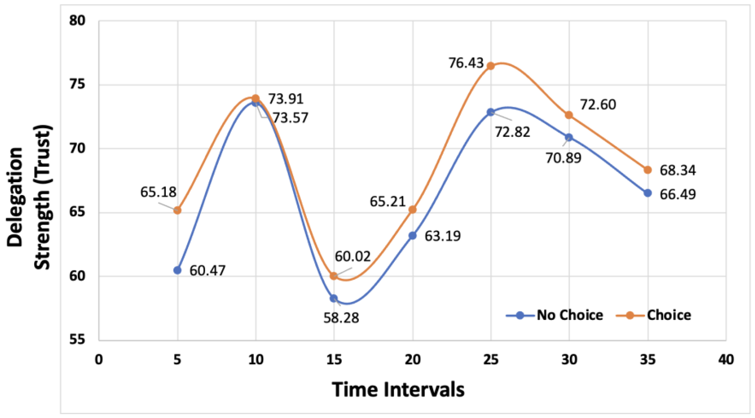
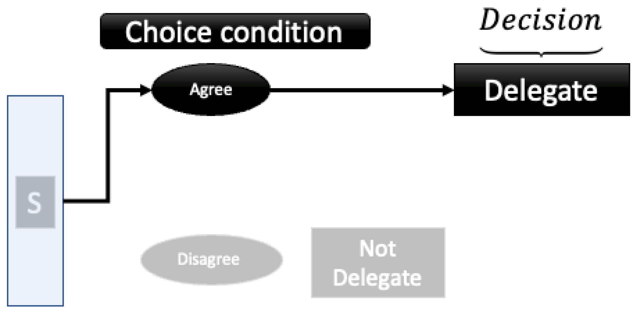
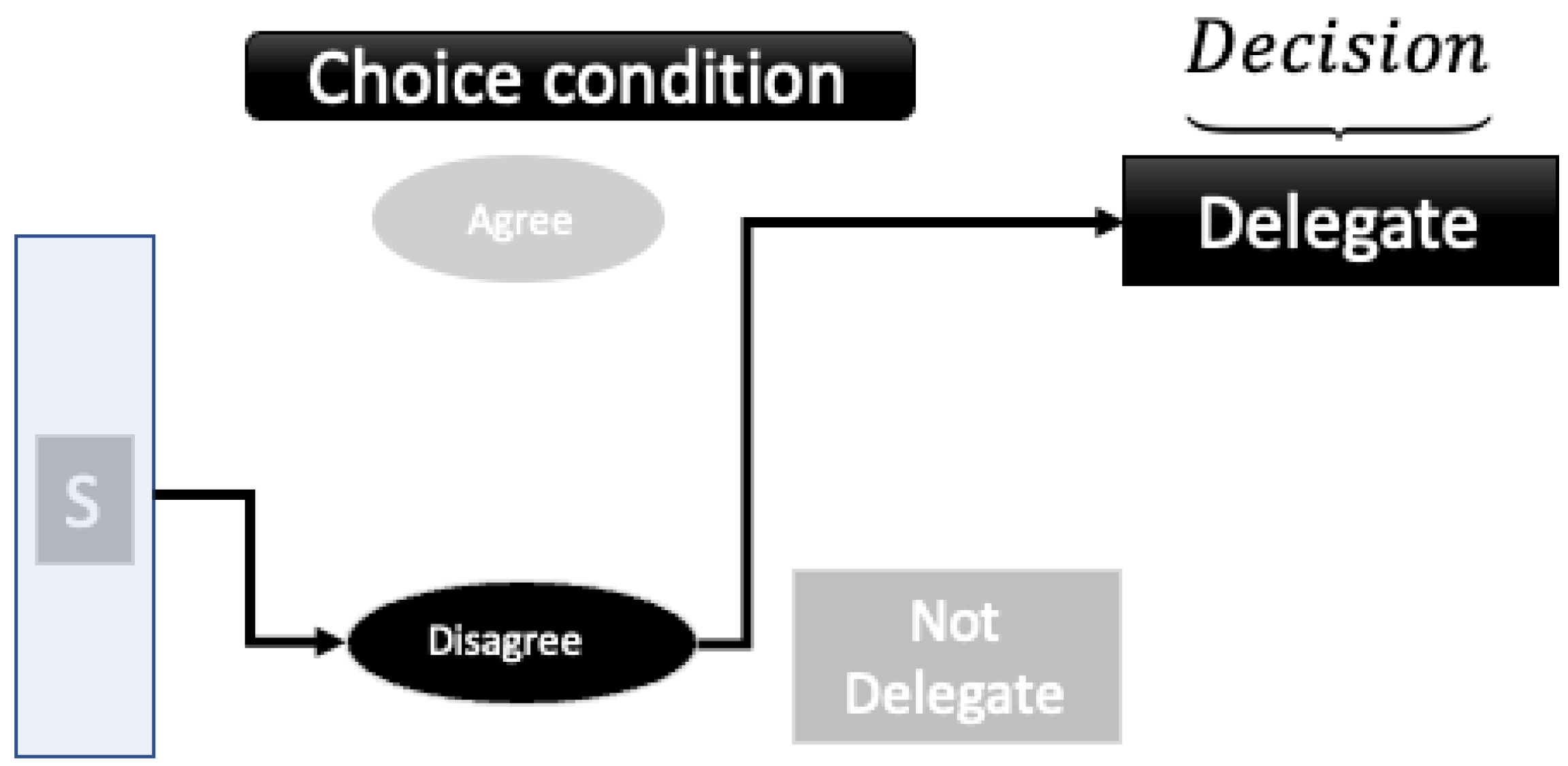
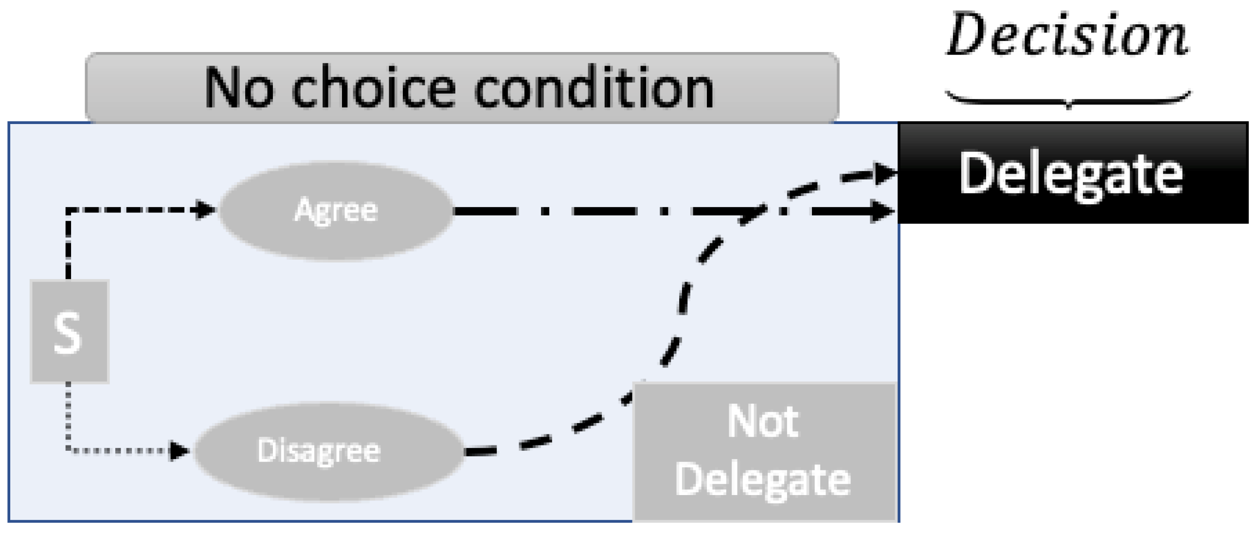


| Categorize, then Delegate Conditions | Delegate Only | ||||||
|---|---|---|---|---|---|---|---|
| Timing | Pr(A) | Pr(Del|A) | Pr(Dis) | Pr(Del|Dis) | TP (Del) Intermediate Judgment | Pr(Del) No Intermediate Judgment | P(Del) |
| 5 Sec | 0.7097 | 0.5966 | 0.2903 | 0.1389 | 0.4637 | 0.4118 | -0.0519 |
| 10 Sec | 0.8495 | 0.7089 | 0.1505 | 0.2143 | 0.6344 | 0.6097 | -0.0247 |
| 15 Sec | 0.6231 | 0.6173 | 0.3769 | 0.2143 | 0.4654 | 0.4559 | -0.0095 |
| 20 Sec | 0.6833 | 0.6042 | 0.3167 | 0.2360 | 0.4875 | 0.4926 | 0.0050 |
| 25 Sec | 0.8566 | 0.7225 | 0.1434 | 0.2895 | 0.6604 | 0.6182 | -0.0422 |
| 30 Sec | 0.8327 | 0.7143 | 0.1673 | 0.1556 | 0.6208 | 0.5941 | -0.0267 |
| 35 Sec | 0.7907 | 0.6716 | 0.2093 | 0.1296 | 0.5581 | 0.5257 | -0.0324 |
| Agree (A) | Disagree (DisA) | |
| Delegate (D) | a | b |
| Not Delegate (notD) | c | d |
| Delegate (D), | e |
| Not Delegate (notD) | f |
| Fit Parameters | |
|---|---|
| 390.45 | |
| 30.12 | |
| 5.95 | |
| 19.62 | |
| 0.21 | |
| Condition | SSE for Quantum Open System Models |
|---|---|
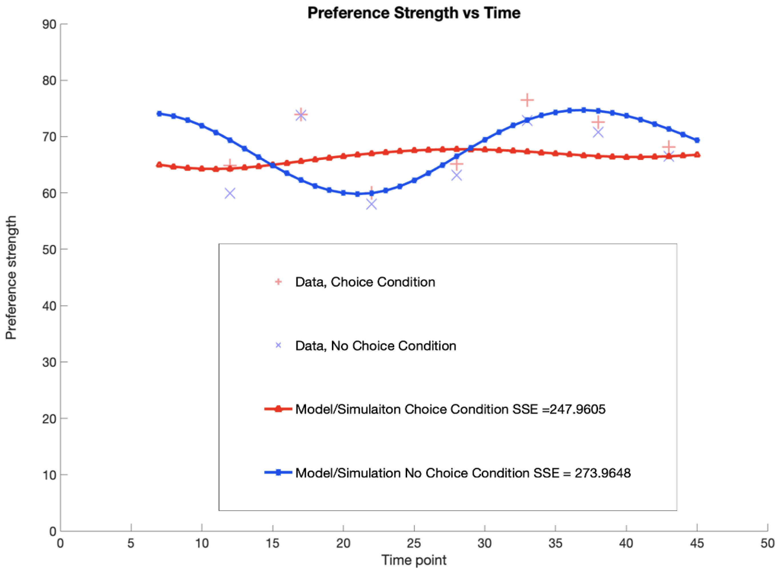
| Choice | 247.9605 |
| No Choice | 273.9648 |
Disclaimer/Publisher’s Note: The statements, opinions and data contained in all publications are solely those of the individual author(s) and contributor(s) and not of MDPI and/or the editor(s). MDPI and/or the editor(s) disclaim responsibility for any injury to people or property resulting from any ideas, methods, instructions or products referred to in the content. |
© 2024 by the authors. Licensee MDPI, Basel, Switzerland. This article is an open access article distributed under the terms and conditions of the Creative Commons Attribution (CC BY) license (http://creativecommons.org/licenses/by/4.0/).


