1. Introduction
Thanks to vertical indoor-farming (VIF) with hydroponics, salads, fruit, vegetables and spices could grow directly in the city in the future. The pioneers of the technology [
1] hope that
vertical indoor-farms (VIFs), also known as
vertical plant factories, can ensure a greater food supply for the rapidly growing world population and will lead to greater sustainability and better flavour. At present, VIF is still a niche market, but it is recognised as an expanding sector.
To date, most vertical plant factories have focussed primarily on the production of leafy vegetables, salads and micro-vegetables, but also many spices/herbs, as their production cycles and environmental requirements are relatively simple. In contrast, there is only a very limited selection of fruit and fruit vegetables that can be grown well in a vertically controlled environment. Fruit plants such as tomatoes, peppers, cucumbers and strawberries, among others, are much more difficult to cultivate than other plants. They need more nutrients, more light and more care than leafy vegetables or herbs [
2].
Chillies are used in countless dishes in many cultures and are appreciated for their flavour and spiciness. There are around 4,000 varieties of chilli worldwide. These are divided into the five varieties: Capsicum annuum, C. baccatum, C. chinense, C. frutescens and C. pubescens. The largest and industrially most important variety is C. annuum [
3], which is considred in this study. Chillies were harvested as early as 8000 BC and were only native to the American continent until the discovery of America in 1492 [
4]. The pods of chilli plants are a rich source of vitamins and contain antioxidants, which are of therapeutic importance in the treatment of metabolic disorders and obesity [
5]. Species of C. annuum can grow up to 1.5 meters tall and their flowers and fruits usually hang downwards. The growth temperature is 25 degrees Celsius [
6].
Chilli plants belong to the nightshade family and are divided into 10 macro-stages according to the BBCH scale (Biologische Bundesanstalt für Land- und Forstwirtschaft, Bundessortenamt und Chemische Industrie), which shows the sequence of the main growth stages. This detailed description covers plant growth from germination to death [
7]. The scale was updated in 2021 by Feldmann et al. [
8]. Paul et al. [
9] divided the chilli plants into three growth stages to examine them for fungal infestation. Paul et al. [
10] divided the growth cycle of pepper plants into 6 stages for image recognition: buds, flowers, unripe, ripe and overripe peppers.
Machine vision systems with convolutional neural networks (CNNs) are used in many areas of modern agriculture, for example, to classify plant varieties, count fruit, detect diseases, localise weeds, automate harvesting or monitor fields [
11,
12]. Many reviews have reported the MV application status in agriculture. They are mainly involved in field crops, for example, [
13], but only a few of them refer to plant factories, for example, [
12].
Automatic monitoring systems are implemented in indoor farms for the visual inspection of plants. The cameras are mounted in a bird’s eye view and are positioned above the plants using moving axes [
14]. For example, the cultivation of seedlings is monitored [
15]. These systems are also used to measure the size of plants with stereo cameras and are suitable for vertical cultivation [
16,
17]. Camera motion systems are also used in the field of plant phenotyping, which quantitatively analyses and measures the external appearance (phenotype) of plants [
18,
19].
You Only Look Once (YOLO) models introduced in [
20] are mainly used in the field of object recognition for fruit detection and achieve very good results in terms of accuracy, processing speed and the processing of high-resolution images [
21]. Coleman et al. [
22] investigated the recognition of cotton growth stages using various YOLO models. The v8x model performed best for recognising the 8 classes considered. Paul et al. [
10] have successfully developed a YOLOv8 model for recognising the growth stages of pepper plants in greenhouses. Their dataset consists of images mainly from the side view, focussed on flowers and fruits. The recognition of growth stages in hydroponic systems has been successfully implemented on lettuce using images from above only [
23].
The challenges that MV systems and algorithms face in VIFs are [
12]:
Changing lighting conditions and complex indoor backgrounds make it difficult for MV algorithms to segment feature areas from images. In addition to the plant itself, there are irrigation pipes, suspension cables, mechanical equipment and other support facilities. The lighting also changes periodically according to the needs of the plants, i.e. growth stages.
There are gaps in the knowledge of the application of MV in specific indoor scenarios, which affect the effectiveness of the technology.
In this paper, the recognition of the growth stages from two configurations: a) the bird’s eye view and b) the combined bird’s eye and side view will be presented and discussed. The effects of the accuracy by extending the datasets with images from the side view as well as the performance of different YOLOv8 model architectures will be investigated. In contrast, state of the art is that camera systems are placed only above the planting bed. The growth stages of the chilli plant are divided into three classes: Growing, Flowering and Fruiting. This categorisation results from the necessary adjustment of the hydroponic system parameters in relation to light and nutrient solution. Furthernore, we install industrial cameras while most of references take digital cameras to get images manually, which inevitably causes uneven und non-producable image quality.
The remaining sections of the paper are organised as follows:
Section 2 describes the experimental setup (hydroponic environment developed for cultivation of chilli plants) and introduces the methods for pre-processing the image datasets, including image acquisition, image data augmentation, the creation of image datasets, and the methods and algorithms (YOLOv8) implemented for the detection of the growth stages of chilli plants.
Section 3 presents the experimental results and comparative analysis. In
Section 4, the results are discussed.
Section 5 provides the conclusions and directions of subsequent work and improvement.
2. Materials and Methods
For the investigation of the growth stages of chilli plants in VIF from a bird’s eye and side views,
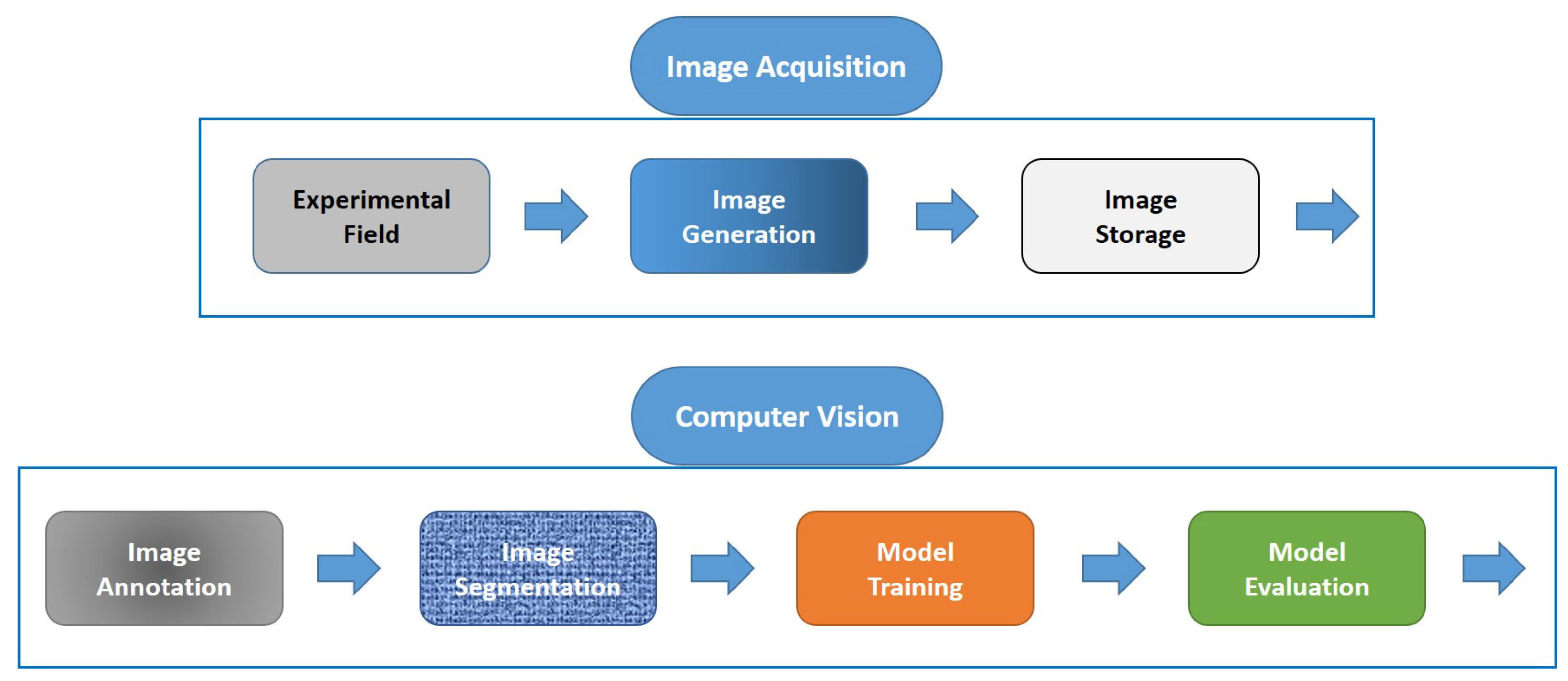
Figure 1 shows the contributions and development scope of this work. The process includes the image acquisition, the experimental setup, the acquisition and storage of images. The next step is the computer vision system, which includes image pre-processing, modeling using DL and evaluation.
2.1. Experimental Field
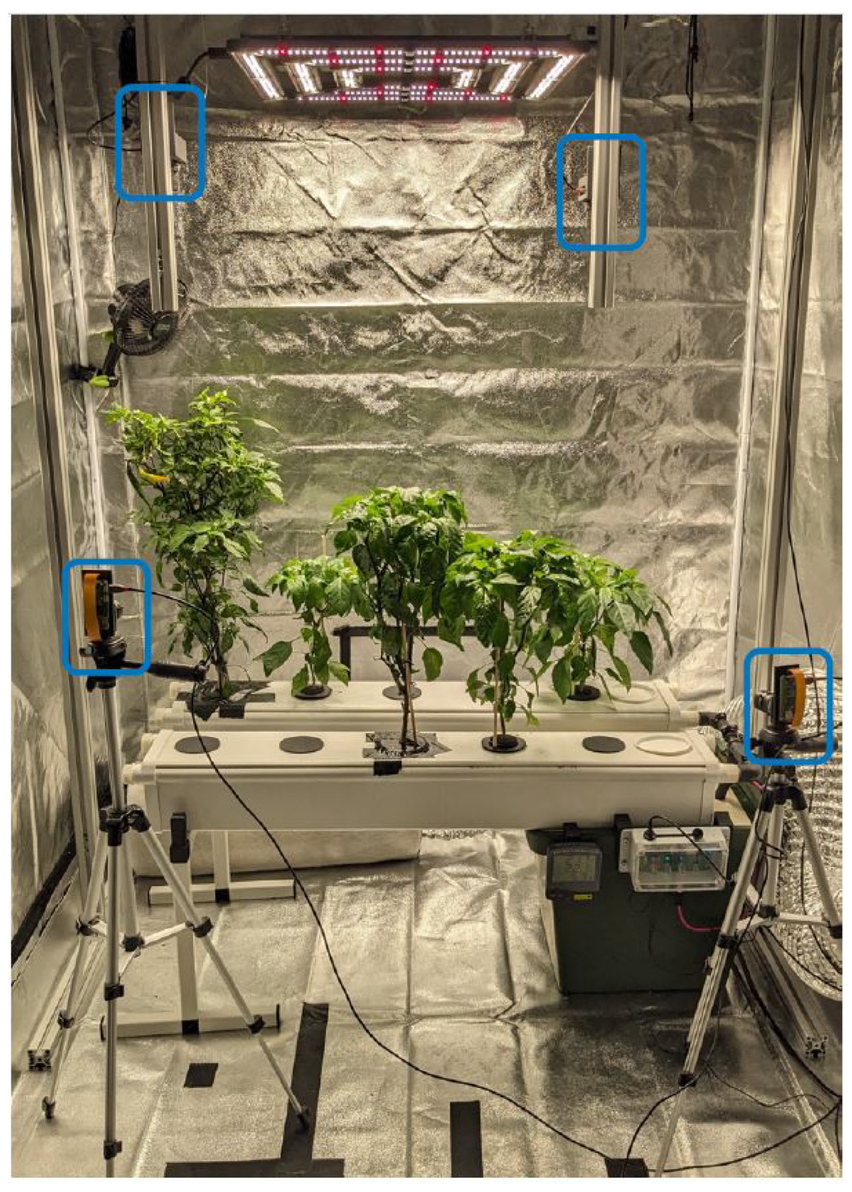
Figure 2 shows the experimental setup with the chilli plants and the four camera systems installed. The overall hydroponics test stand system developed consists of several subsystems: Essentially, a hydroponics system (including the nutrient system), a lighting system, sensor systems and a hydroponics kit are integrated in a cultivation box. The experiments presented in this work are carried out in the CAISA Lab at the Cologne University of Applied Sciences (TH Köln). The DiamondBox Silver Line SL150 [
24] grow box is used for the trials. The dimensions of the system are 1500 mm in width, 1500 mm in depth and 2000 mm in height.
2.1.1. Hydroponics System and Planting
Plant growth requires a controlled working environment so that the growth parameters can be permanently checked and guaranteed. This includes the monitoring of temperature and humidity in the atmosphere as well as an even air flow. pH and EC measurements are used to control the nutrient solution and the photoperiod can be adjusted.
The hydroponic system used is the GrowStream10 V2 NFT system from Terra Aquatica, which is particularly suitable for growing chilli plants [
2]. It consists of two double-walled plastic troughs, in each of which five plants can be placed. The storage container for the nutrient solution has a capacity of 45 litres. The overall dimensions of the system are 1130 mm in length, 460 mm in width and 530 mm in height. For the light supply, which is essential for photosynthesis, the Lumatek ATTIS ATS 300 W PRO LED is used, which is designed for a cultivation area of 1
. A GHP Profan clip fan is used to ensure the necessary air circulation within the grow box.
The composition of the nutrient solution is based on an N-P-K ratio of 3-1-3 (nitrogen—N-phosphoric anhydride—P2O-potassium oxide—K2O). Both the dry fertiliser Peters Professional Grow-Mix and the liquid fertiliser Terra Aquatica TriPart are used for fertilisation. Terra Aquatica pH-Down and pH-Up are used to regulate the pH value. A disinfectant concentrate is added to the nutrient solution as a prophylactic measure to prevent algae growth. The transplanted areas are sealed with a 3D-printed lid to prevent the penetration of light, which would promote algae growth.
The pH value for growth is kept between 5.8 and 6.5 and the EC value between 1.4 and 1.8 mS/cm. These values, including the temperature of the nutrient solution, are automatically controlled by Atlas Wi-Fi Hydroponics Kit and manually regulated. The light intensity is measured with a Quatum PAR Light Meter from Lightscout at the top edge of the net baskets, which are located in the plastic gutter. The PPFD (Photosynthetically Active Photon Flux Density) value at a height of 14 cm is 257 µmol/s and at a height of 58 cm 584 µmol/ (verified by measurements). The photoperiod is set to 9 hours until the first flowering and to 12 hours for further growth. A combination meter displays humidity and temperature.
2.1.2. Camera Systems
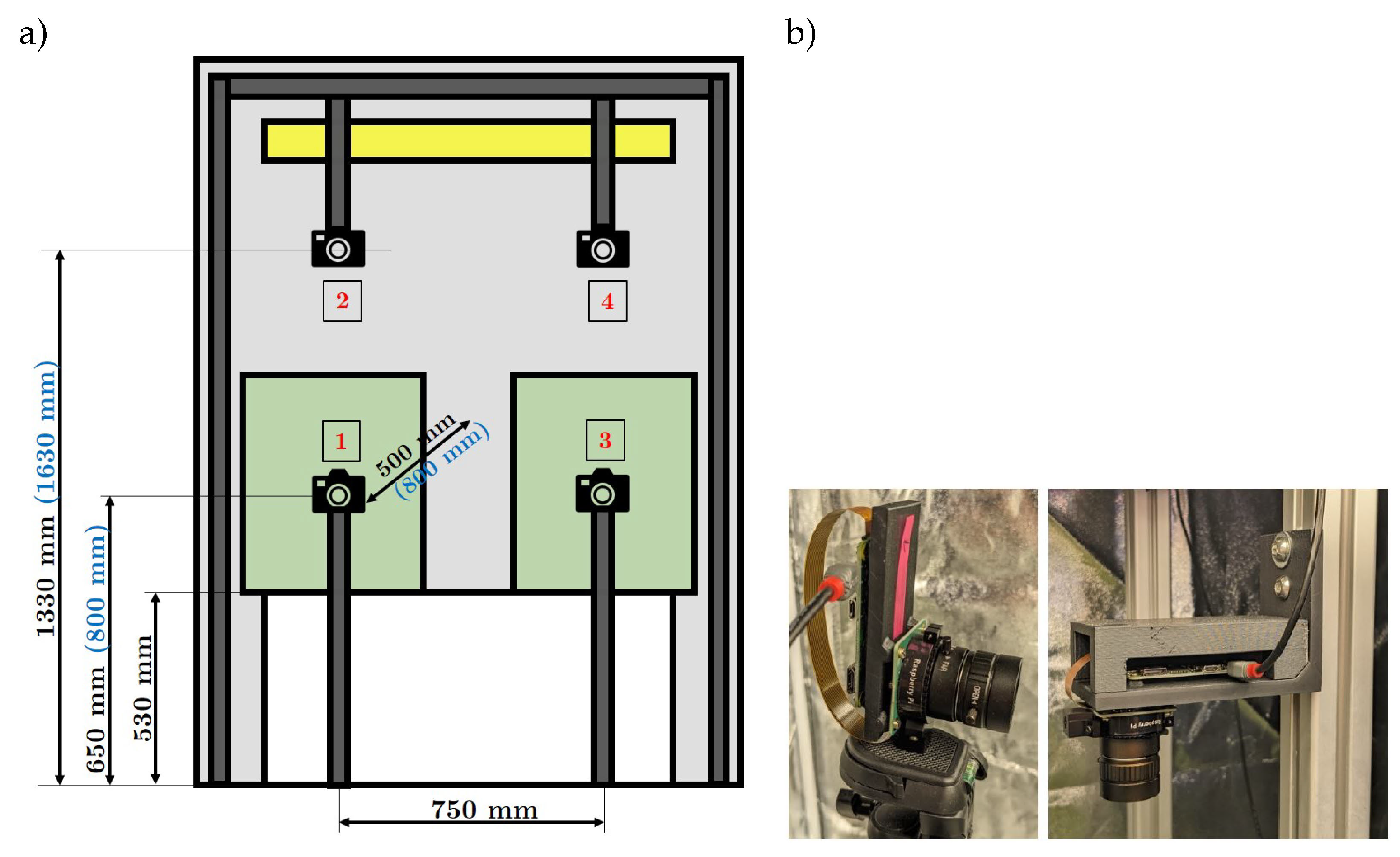
In order to train a machine learning model effectively, a suitable dataset must be created. In the field of computer vision, the data consists of images. In order to generate a large number of images, four cameras are placed in the grow box. Two cameras are used for the bird’s eye view and two cameras for the side view. As shown in the schematic system setup in
Figure 3, the distances between the cameras and the chilli plants to the chilli plants depend on the respective growth stages. The system has been designed to record and store images of at least two chilli plants over their entire life cycle and to consider the changing plants in their entirety, as they can reach a height of between 500 and 700 mm and a width of 300 to 400 mm. To ensure sharp images during growth, flexible positioning of the camera systems is possible.
A plant with its countless leaves, flowers and fruits is a complex representation. To train a deep learning model, it needs a detailed representation of the object. The HQ Raspberry Pi camera with a 12 megapixel camera with a 1/4" (3.2 mm) image sensor is used for this application. The sensor size B, the object width g and the object size G are of central importance for the design of the lens. These values can be used to calculate the focal length of the lens using the BB formula . The expected plant height or object size G is 300 mm in the growing phase and 600 mm from the flowering phase onwards. The object width g is set at 500 mm in the first phase and 800 mm from the second phase onwards. The object distance g for the cameras from the bird’s eye view is set to a maximum of 500 mm. This results in a focal length f of 5.28 mm and 4.24 mm. A 6 mm wide-angle lens is available for the HQ Raspberry Pi camera. To process and save the images, the camera system is connected to the the compatible Raspberry Pi Zero W single-board computer, including 32 GB memory card.
The camera system for the side view (camera system 1 and 3) is attached to a height-adjustable travelling stand using a mounting bracket, as shown in
Figure 3a. For the bird’s eye view camera system (camera systems 2 and 4), a frame made of aluminium profiles is positioned inside the grow box. Two perpendicular profiles are mounted on the cross strut, to which the mounting bracket for the camera system is attached, as illustrated in
Figure 3b.
Table 1 lists the components required for the camera system, including the Raspberry Pi 4 B for the central image storage and network cable for the power supply.
2.2. Image Data Acquisition
Image acquisition is controlled via the Raspberry Pi Zero W using a Python script. The image resolution is set to the maximum value of pixels, which is limited to 3 megapixels by the lens. Due to the mounting position of camera systems 2 and 4, the images are rotated 180 degrees to ensure correct image alignment. The images are then triggered. Four images are taken and saved by the camera systems throughout the day. The recordings are carried out at 9:00 am, 11:00 am, 1:00 pm and 3:00 pm. The trial period of the recording extends from 9 August to 7 Deecmber 2023.
2.3. Image/Data Pre-processing
The recorded and saved images are available as raw data. Before they are used for model calculation, some data pre-processing steps are necessary, such as annotation and augmentation of the images as well as appropriate dataset splitting for model training, testing and validation.
2.3.1. Image Annotation
Object recognition involves class identification and localisation in an image. In a supervised learning setting, annotations are used to tell the model which of the Growing, Flowering and Fruiting classes is present and where it is located in the image. During object recognition, a rectangular bounding box is drawn around the object to define its position. A class assignment is then made. These meta data have a clear assignment and serve the model as the basis for the prediction.
The annotation is carried out using Roboflow [
25], a freely accessible web application that provides tools for annotation and comprehensive calculations for tasks in the field of computer vision. The images are uploaded to Roboflow and the annotation tool is used to mark the area of the image where the chilli plant is located with a bounding box. The number of bounding boxes is based on the number of objects in the image. Roboflow also converts the images to 640 x 480 in order to optimise computing power and retain a sufficient level of detail.
2.3.2. Image Augmentation
Augmentation makes it possible to increase the number of existing images in order to provide more training data for the model. This involves changing the images, for example by mirroring or rotating them. Augmentation is only carried out on the training data. This is to prevent similar images from appearing in the training, test and validation dataset, as only unmodified images enable a real performance assessment. It is crucial that the generated bounding boxes and their coordinates are also adapted to the changed conditions. The position of the object within the image can change as a result of the augmentation.
In this study, three transformations were applied:
Flipping the image on the horizontal axis.
Rotating the image by an angle up to 40 degrees selected randomly from the uniform distribution.
Randomly changing the brightness and contrast of the image.
The open source library Albumentations [
26] has been used for implementing these options. The parameter
is set for the probability of the augmentation being applied.
Figure 4 shows examples after augmentation. The pipeline is run three times per image and generates a three times higher image dataset with random augmentations from the raw data.
2.3.3. Datasets
The datasets serve as the basis for model training. Two datasets for images have been created: one dateset from the bird’s eye view (BV) and another from the bird’s eye and side view (BSV).
Before augmentation, the image data are divided in a ratio of 70-10-20. As most of the data are required for training the model to learn features and patterns, 70% of the data is used for this. After each complete run of the calculation on the training dataset, the model is tested on the validation dataset. This is to prevent over-fitting to the training data. For this purpose, 10% of the data that is not included during training is used. In order to obtain unbiased test results of the trained model, 20% of the data is withheld for the test dataset. As the validation data are already used during training, unused data are crucial for the evaluation. The test evaluation only takes place on the test set (BV) for all trained models from the bird’s eye view and bird’s eye and side view. The reason for this is the performance comparison of the two models for the data from the bird’s eye view.
The raw dataset from the bird’s eye and side view consists of a total of 1489 images, of which 742 images from the bird’s eye view and 747 images from the side view. After augmentation, the dataset consists of a total of
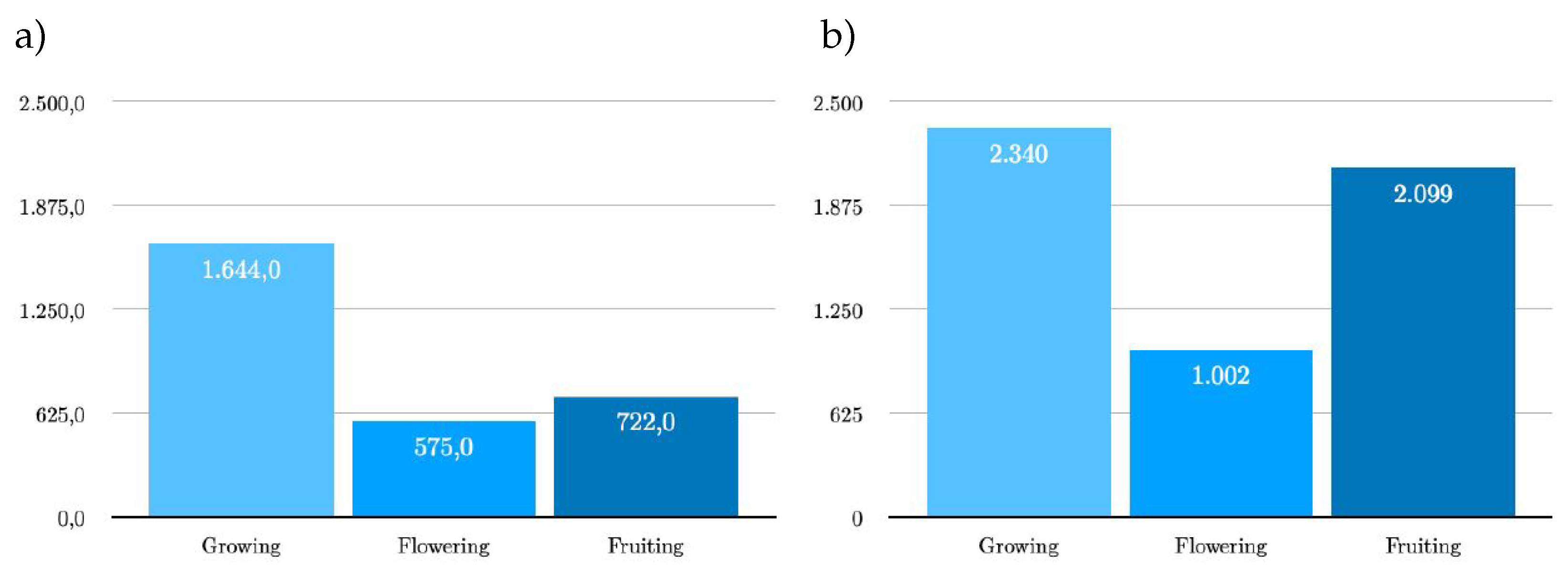
bird’s eye view consists of a total of 1780 images with 2941 labels (bounding boxes). Since only the training dataset was extended by augmentation, the ratio to 88-4-8 training ratio changes to 88-4-8 training, validation and test images. As can be seen on the left in
Figure 5, the Growing class contains 1,644 labels, Flowering 575 and Fruiting 722 labels. The original dataset for the
bird’s eye and side view comprises 3,573 images. As the test dataset is identical to that of the bird’s eye view, the total dataset consists of 3,423 images with a total of 5,441 labels. The new ratio of training, validation and test dataset is 90-5-5. The Growing, Flowering and Fruiting classes contain 2,340, 1,002 and 2,099 labels respectively, as shown in the bar chart on the right in
Figure 5.
The distribution of the labels for the training, validation and test data depending on the views and the classes Growing, Flowering and Fruiting can be seen in
Table 2.
2.4. Detection and Classification Methods and Tools
2.4.1. Model Training Procedurce
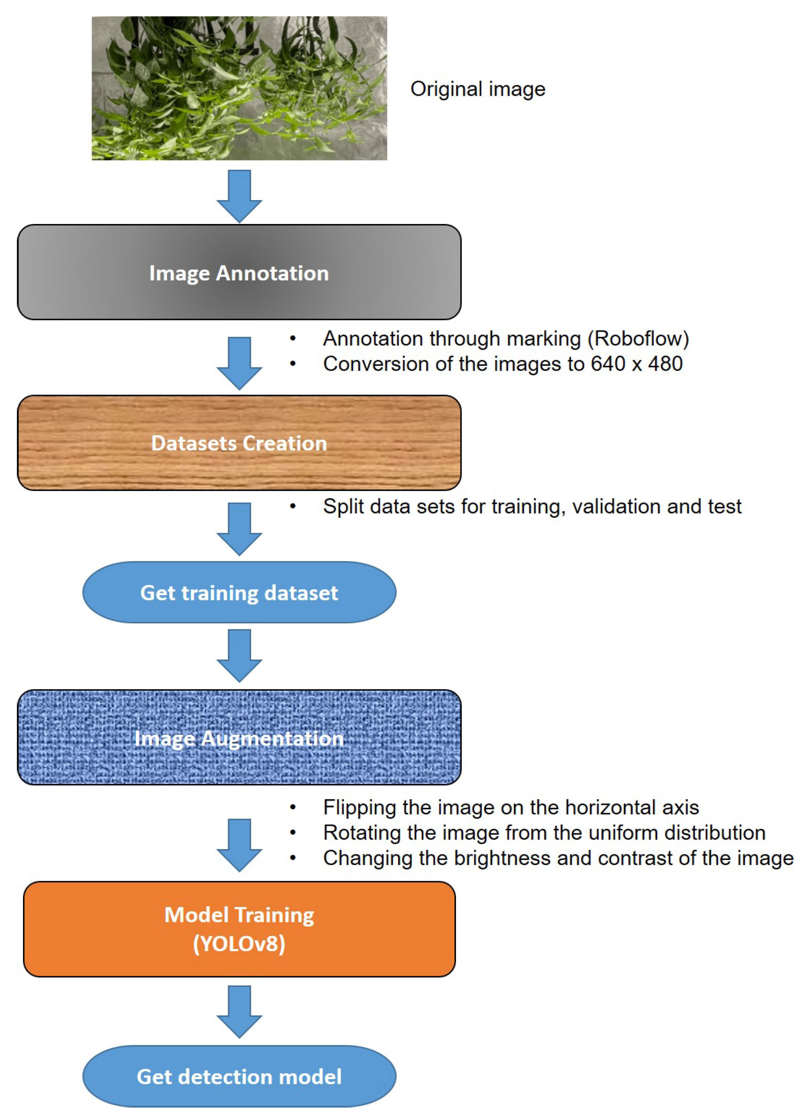
The third part of the computer vision pipeline (
Figure 1) consists of the calculation of the model. The YOLOv8 model [
27], a deep learning model developed based on Ultralytics, is used for the task of recognising the growth stages, as it is currently regarded as the most powerful model for the recognition of objects of full sizes for the following reasons [
28]: (a) lightweight network architecture, (b) effective feature fusion methods, (c) and more accurate detection results than its predecessor versions YOLOv3–YOLOv7. The training process of growth stage detection procedure is shown
Figure 6.
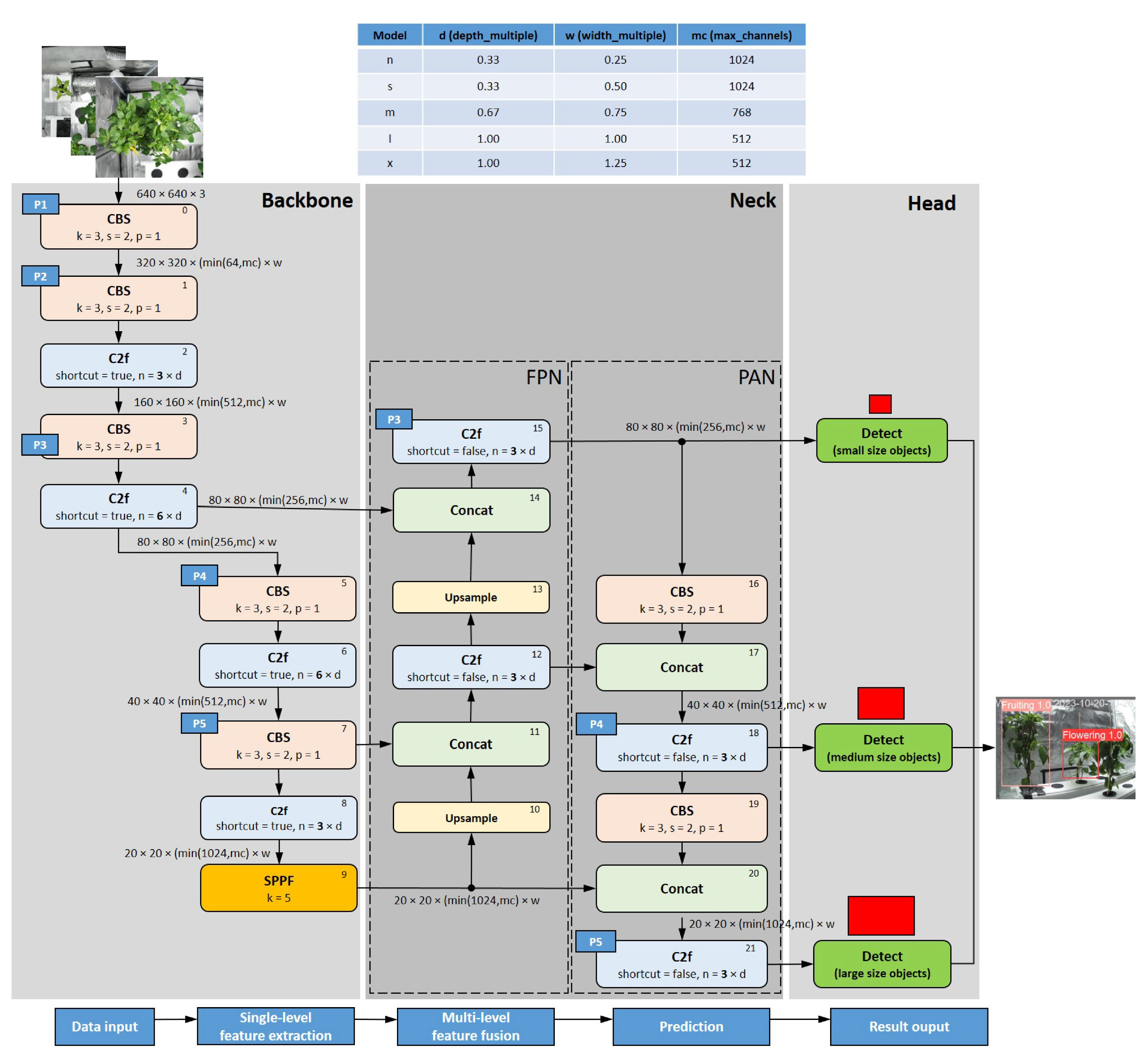
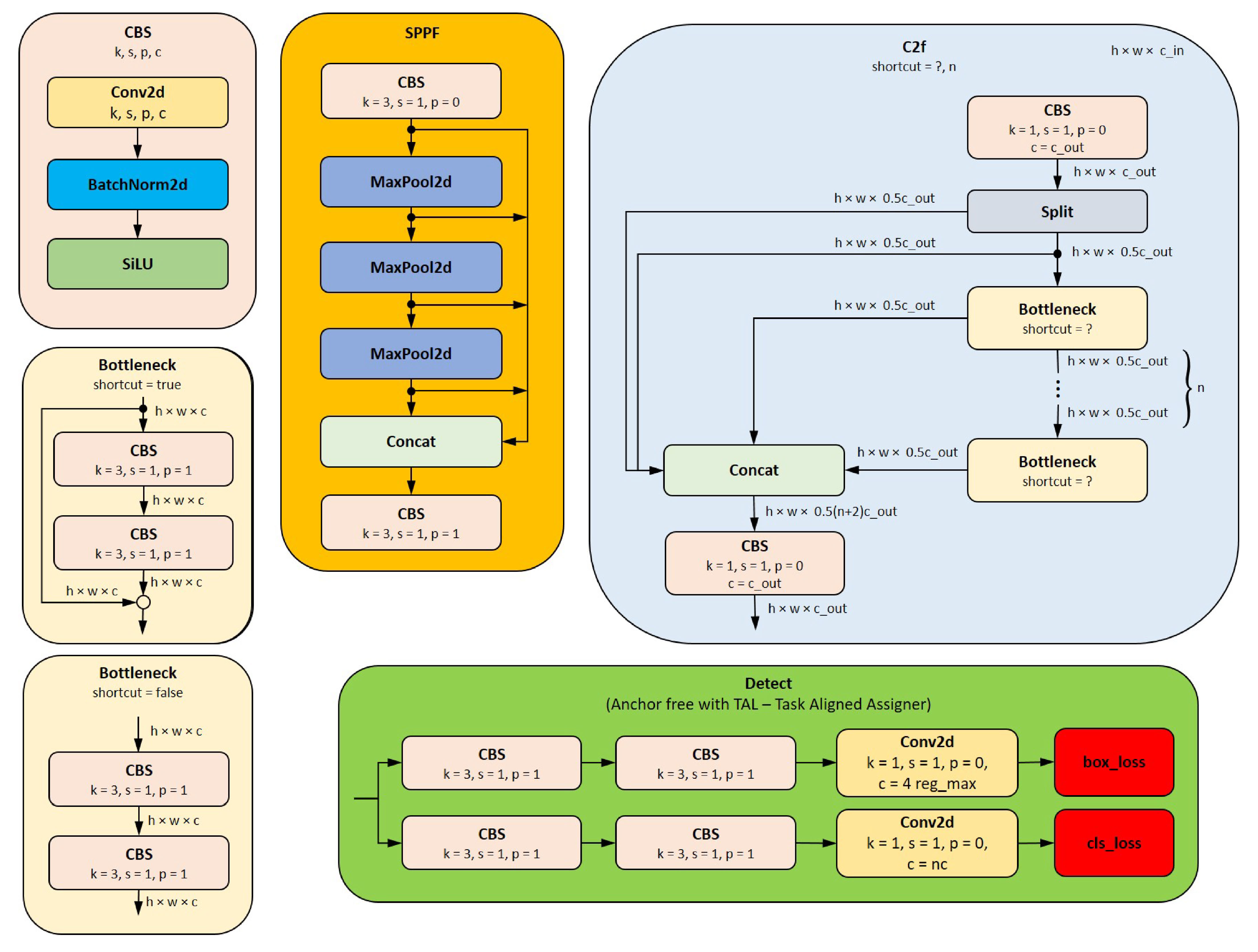
The YOLOv8 network structure consists of three main parts (see
Figure 7 and
Figure 8):
The
backbone is basically the same as that of YOLOv5 and consists of a series of convolutional and deconvolutional layers to extract features. It also incorporates residual connections and bottleneck structures to reduce network size and improve performance [
29]. This part uses the C2f module as the basic building block that replaces the C3 module in YOLOv5. This offers better gradients to support different model scales by adjusting the number of channels. At the end of backbone, an SPPF module is used, and three Maxpools of size
are passed serially, and then, each layer is concatenation, so as to guarantee the accuracy of objects in various scales while ensuring a light weight simultaneously [
28].
The
neck part uses multi-scale feature fusion techniques to merge feature maps from different stages of the backbone to improve feature representation capabilities. The feature fusion method used by YOLOv8 is still PAN-FPN [
30,
31], which strengthens the fusion and utilization of feature layer information at different scales. Two upsampling and multiple C2f modules together with the final decoupled head structure are used to compose the neck module. The idea of decoupling the head in YOLOvx, is used by YOLOv8 for the last part of the neck. It combines confidence and regression boxes to achieve a new level of accuracy [
28].
The
head, which is responsible for the final object detection and classification tasks, adopts a decoupled head structure, separating the classification and detection heads branches. The detection head consists of a series of convolutional and deconvolutional layers to generate detection results, while the classification head uses global average pooling to classify each feature map. It also adopts an anchor-free strategy, abandoning the anchor boxes used in YOLOv7, which reduces the number of box predictions and improves the speed of Non-Maximum Suppression (NMS) [
29]. For loss computation, YOLOv8 uses the Task Aligned Assigner positive sample assignment strategy. It uses BCE Loss for the classification branch and Distribution Focal Loss (DFL) and CIoU Loss for loss computation in the regression branch. YOLOV8 requires decoding the integral representation of bbox shapes in Distribution Focal Loss, using Softmax and Conv computations to transform them into conventional 4-dimensional bboxes. The head section outputs feature maps at 6 different scales. The predictions from the classification and bbox branches at three different scales are concatenated and dimensionally transformed. The final output includes three feature maps at scales of
,
and
(inputs of the "Detect" blocks in
Figure 7).
YOLOv8 is available in five variants, which differ mainly in the number of convolutional layers: YOLOv8n (nano), YOLOv8s (small), YOLOv8m (medium), YOLOv8l (large) and YOLOv8x (extra large). In this study, the three variants
YOLOv8n,
v8m and
v8l are used to analyse the two datasets (see
Section 2.3.3). Smaller models, which are represented by the YOLO variants, require less computing power for the prediction of unknown data. Larger architectures, such as YOLOv8l, are more accurate but require more computing power. The present results should serve as a guide in the future to better understand the required computing power depending on the accuracy requirements.
Figure 7.
YOLOv8 network structure. Legend: CBS – Convolution + Batch Normalisation + Sigmoid-weighted Linear Unit (SiLU); C2f – CSP (Cross Stage Partial) bottleneck with 2 convolutions, Fast version; SPPF – Spatial Pyramid Pooling, Fast version; Concat – Concatenation,; Detect: Detector; FPN – Feature Pyramid Network; PAN – Path Aggregation Network. See
Figure 8 for representation of the subblocks used.
Figure 8.
YOLOv8 architucture subblocks used in
Figure 7. Legend: SiLU – Sigmoid-weighted Linear Unit; Conv2d – 2D convolution; BatchNorm2d – 2D Batch Normalisation; Maxpool2d – 2D max pooling; box_loss – (bounding) box loss; cls_loss – class loss.
Figure 8.
YOLOv8 architucture subblocks used in
Figure 7. Legend: SiLU – Sigmoid-weighted Linear Unit; Conv2d – 2D convolution; BatchNorm2d – 2D Batch Normalisation; Maxpool2d – 2D max pooling; box_loss – (bounding) box loss; cls_loss – class loss.
2.4.2. Model Parameters
There are a large number of parameters for customising and controlling the YOLO models, which can be modified on an individual basis. These include organisational aspects, such as the management of the storage location and the naming of the project, as well as hyperparameters that can have a decisive influence on the accuracy and speed of the trained model.
The calculations in this work are largely carried out using the standard parameters.
Table 3 shows the most important hyperparameters for the calculation:
The number of epochs indicates how often the entire training dataset was run through the YOLOv8 algorithm. 300 epochs are selected to ensure adaptation on the one hand and not to overstretch the calculation time on the other.
The batch size specifies how many parts the training dataset is divided into. After each run, the model performance is adjusted to improve the learning performance. One epoch corresponds to the run of all batches. 16 batches are selected for the application, as smaller batches lead to faster convergence, but are subject to greater fluctuations. Larger batches lead to more accurate estimates, but require more storage capacity and therefore computing power.
The image size refers to the dimensions of the images in width and height that are processed by the model. Higher resolutions require more computing resources, smaller resolutions can lead to a loss of information. As this task involves small details such as buds, blossoms and fruit buds, an image format of 640 x 480 is selected. YOLO models process images in a 1:1 ratio, so the shorter side of the image is filled with black bars to maintain the original ratio.
The models obtained were pre-trained on the COCO dataset [
32]. These models have already developed the ability to recognise features and patterns. The COCO dataset, which contains a total of 80 classes, also includes the "potted plant" class. In order to compare the models but stay within the limits of computational resources, the YOLOv8n, v8m and v8l models are used.
Table 3.
Information on the hyperparameters for the calculations.
Table 3.
Information on the hyperparameters for the calculations.
| Epochs |
Batch Size |
Image Size |
Model |
| 300 |
16 |
|
YOLOv8n |
| |
|
|
YOLOv8m |
| |
|
|
YOLOv8l |
2.4.3. Computation Environment
The setup for the calculation consists of a Dell Precision 3660 workstation with Central Processing Unit (CPU) Intel Core i9-13900, a Random Access Memory (RAM) of Memory (RAM) of 64 GB and the Graphical Processing Unit (GPU) from NVIDIA RTX A5000, as can be seen in
Table 4. The calculation is performed in the Integrated Development Environment (IDE) Visual Studio Code with Python version 3.11.5 is used.
2.5. Performance Evaluation Metrics
There are different approaches for evaluating the object recognition models. The
Intersection over Union (
) is a value between 0 and 1 that describes the overlap between the predicted bounding box and the ground truth, the actual bounding box, as shown in the formula [
33]:

An IoU value of 1 means complete overlap, while a value of 0 indicates that the boxes do not touch at all. Each bounding box that is recognised can be assigned to one of the four components listed in
Table 5.
The classification results of each image can be visualised using a confusion matrix. This matrix illustrates the extent to which the predicted classes correspond to the actual ground truth classes. Values such as precision, recall and F1 score can be derived from this.
Precision (
P) evaluates the proportion of correct positive predictions in relation to all positive predictions and shows the ability of the model to minimise false positive results, as the following formula shows:
Recall (
R) is the proportion of correct positive predictions in relation to all actual positive instances and evaluates the ability of the model to recognise all instances of a class. This is calculated as follows:
Precision-Recall curve (PR curve) is a graph that shows precision values on the
y-axis and recall values on the
x-axis. High precision and recall values are a positive indication of the model.
Average Precision (
) is the area under the PR curve.
Mean Average Precision (
) is the average of the AP values across all classes and is calculated as follows:
where
denotes the AP value for the
ith class, and
C the total number of classes contained in the dataset. This is useful in scenarios with multi-class object recognition to enable a comprehensive evaluation of model performance [
33].
Loss functions play a decisive role in the context of training a model for object recognition. These functions are used to determine the difference between the predicted bounding boxes and the actual annotations. They provide information on how effectively the model learns during training. Typical components of loss functions are the
bounding box loss (
box_loss), the
class loss (
cls_loss) and
defocus loss (
dfl_loss).
box_loss takes into account the error in the coordinates of bounding boxes in the prediction. The aim is to get the model to match the predicted bounding boxes to the ground truth boxes.
cls_loss measures the deviation in the prediction of the object class for each bounding box. This ensures precise identification of the class of the object.
dfl_loss is used to optimise object recognition with blurred or defocused images [
34].
3. Experimental Results and Comparative Analysis
The last step of the computer vision pipeline in
Figure 1 involves evaluating the models. In this section, the results of YOLOv8n, YOLOv8m and YOLOv8l are presented using the bird’s eye view and bird’s eye and side view datasets. The metrics described in
Section 2.5 serve as benchmarks for comparison between the models.
3.1. Image Recordings
The raw dataset of all image recordings comprises 1489 images that were generated with the four camera systems. The data collection period spanned four months, with the camera systems generating the images throughout the day (see
Section 2.1).
Figure 9 presents images of the growth stages—from left to right, the growing, flowering and fruiting phases can be seen from a bird’s eye view.
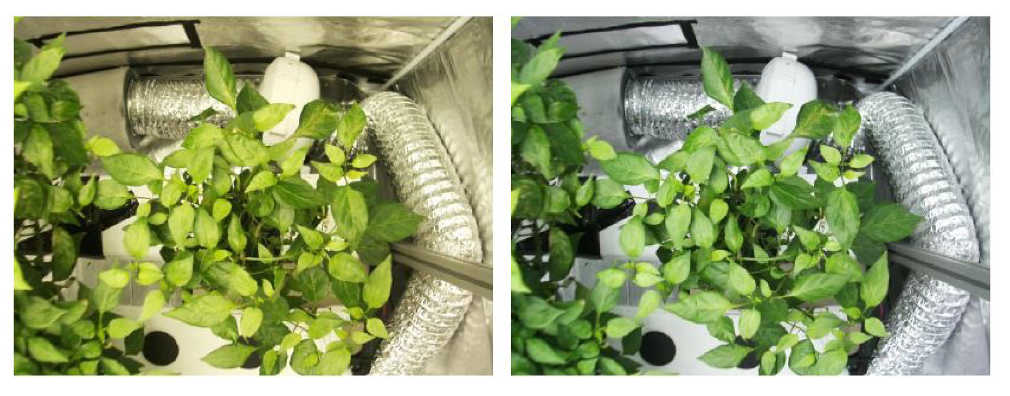
The colouring of the images from the side view reflects the prevailing conditions in the grow box. In contrast, the images from a bird’s eye view, especially during the flowering and fruiting stages of growth, have a yellowish tinge.
Figure 10 shows an image of a plant taken on the same day, with a yellowish cast visible on the left-hand side, while the right-hand side is unaffected. This only occurred when the front of the grow box was closed. As the lens settings were made with the grow box open, the camera system did not adapt to the changed lighting conditions. This lack of white balance led to the yellowish discolouration of the images.
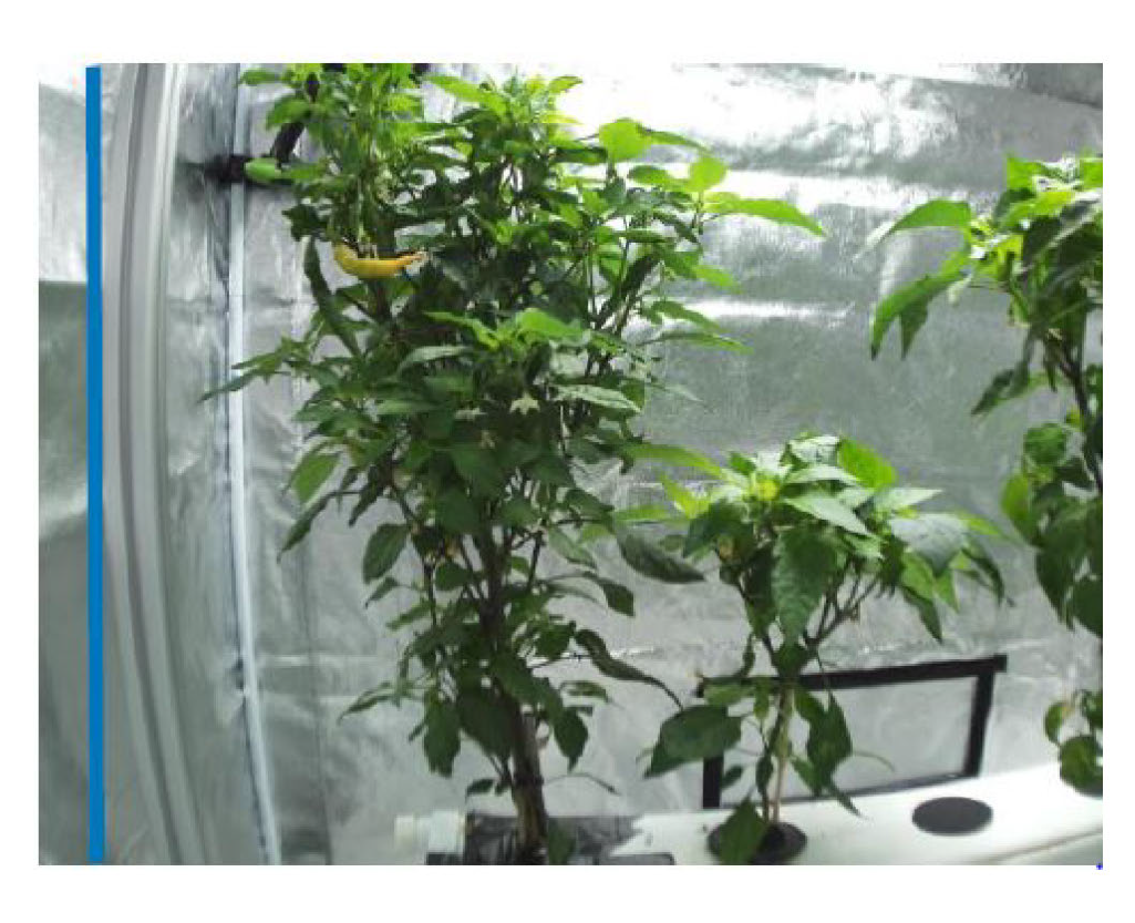
The image recordings of all camera systems show a distortion at the edge of the image. This barrel distortion is clearly recognisable in
Figure 11, particularly at the left edge of the image on the basis of the frame. The course of the frame is curved inwards, which is emphasised by the vertical blue line. At short focal lengths, this distortion occurs mainly with wide-angle lenses. The distance between the camera lens and the plants is determined by the dimensions of the grow box.
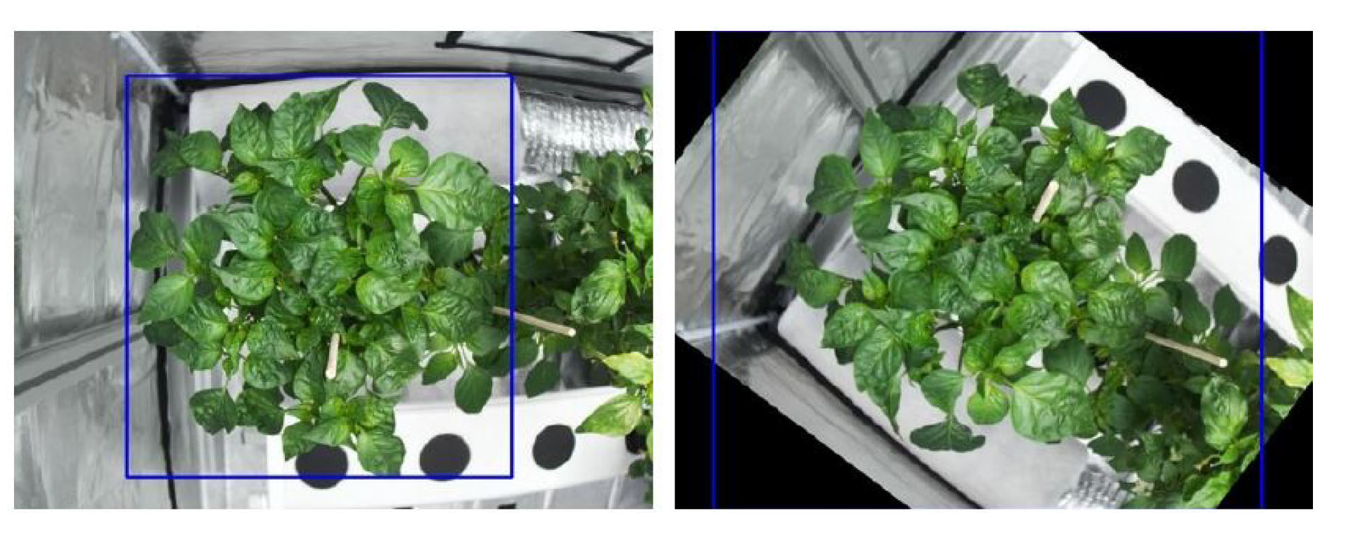
Augmenting the images made it possible to enlarge the dataset. With large rotations of the images, the bounding boxes are expanded, as can be seen on the right of
Figure 12. In contrast, the bounding box on the unprocessed left-hand image is closely aligned with the canopy of the plant.
3.2. Model Training Results
All calculations were carried out under the hardware conditions described in
Section 2.4.3. The evaluation metrics of the training results are the loss functions and the
values as described in
Section 2.5. The loss functions provide information about the inaccuracy of the predictions. The
values provide insights into the classification and localisation of the objects in the model. Both the
and
values are considered here, whereby these differ in their
threshold value. The
value refers to the calculation of an
threshold value of 0.5, while the
value takes into account various
threshold values from 0.5 to 0.95 in 0.05 steps. The test results are additionally described with a confusion matrix and precision and recall are given.
For clear identification, the models with the bird’s eye view training dataset are labelled with a BV (YOLOv8n-BV, YOLOv8m-BV, YOLOv8l-BV) and those with the side and bird’s eye views with a BSV (YOLOv8n-BSV, YOLOv8m-BSV, YOLOv8l-BSV).
3.2.1. Training Results Bird’s Eye View
The YOLOv8n-BV model consists of 3.01 million parameters and 225 layers. Under the hardware conditions described, training for all 300 epochs takes 35 minutes. The finished model size is 6.3 MB.
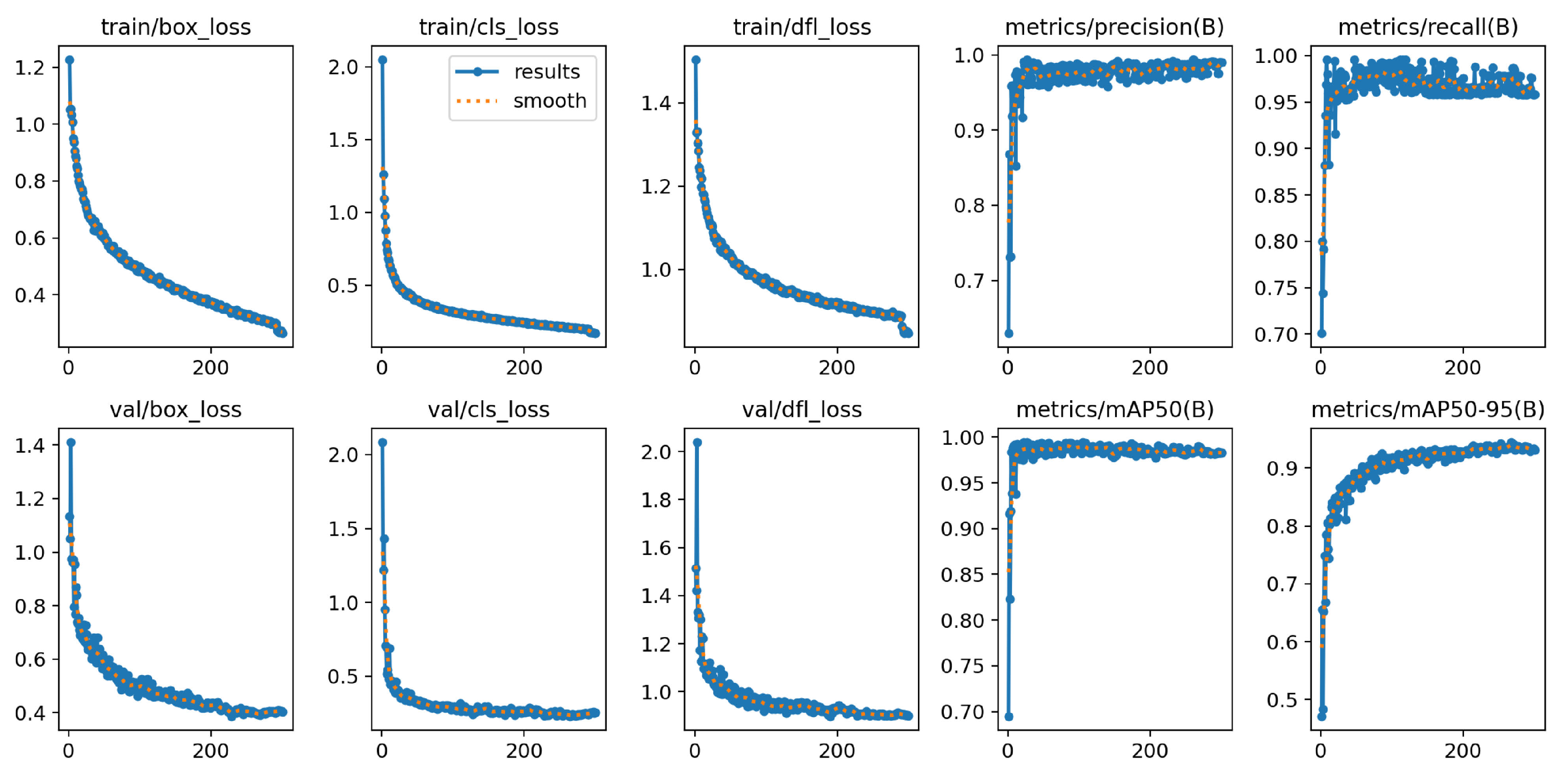
Figure 13 illustrates the overall results of the model calculation over all epochs, with the loss functions during training and validation, the
and
, as well as the precision and recall curve. The graphs of the loss functions decrease steadily over the training epochs. A sudden drop in the
and
can be recognised in the last 10 epochs. The validation curves drop sharply at the beginning and then stabilise at a low level. The
curve converges after a few epochs and the
graph shows an exponential convergence.
The
value of the model on the validation data is 99.0 % and the
value is 94.4 %.
Table 6 shows the distribution of the
values across the three classes Growing, Flowering and Fruiting. The
values of all classes are very high and are separated by a maximum of 1.0 %. Flowering and Fruiting achieve higher
values (96.6 % and 96.5 %) than Growing (90.1 %).
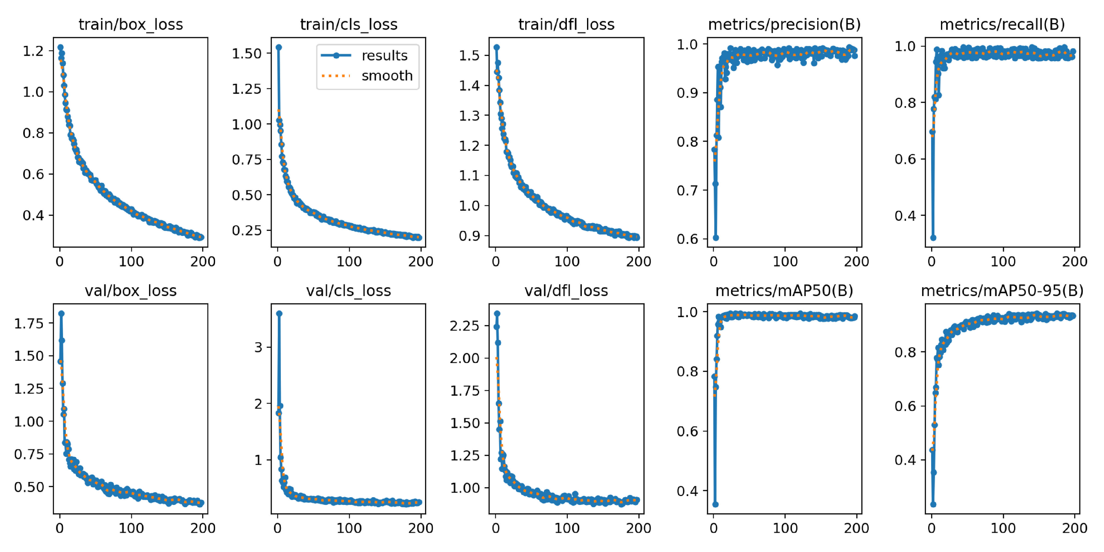
Since the training of YOLOv8m-BV did not show any improvements over the last 50 epochs of validation losses, the training stopped early after 197 epochs. The calculation for the included 25.85 million parameters and 295 layers thus took 1 hour and 2 minutes. The model size of YOLOv8m-BV is 52 MB. The graphs of the
values in
Figure 14 show similar curves to YOLOv8n-BV across all epochs. The loss functions of the training decrease sharply after the first epochs and then change to a constant decrease. On the validation data, the losses are also strongly decreasing at the beginning and then converge to a minimum.
The YOLOv8m-BV model achieves an
value of 99.0 % and an
value of 94.2 % across all classes on the validation dataset, as can be seen in
Table 7. With regard to the
, the values of the individual classes show only slight differences, with Growing achieving the lowest value of 98.0 %. Growing also achieves the lowest value for
at 89.9 %, while Fruiting achieves the highest value at 97.0 %.
The validation of the model across all classes achieves an
value of 98.9 % and an
value of 94.8 %. Looking at the individual classes, Flowering and Fruiting have the same
value of 99.5 % and Growing 97.8 %. Growing, Flowering and Fruiting achieve an
value of 91.0 %, 95.8 % and 97.6 % respectively, as can be seen in
Table 8.
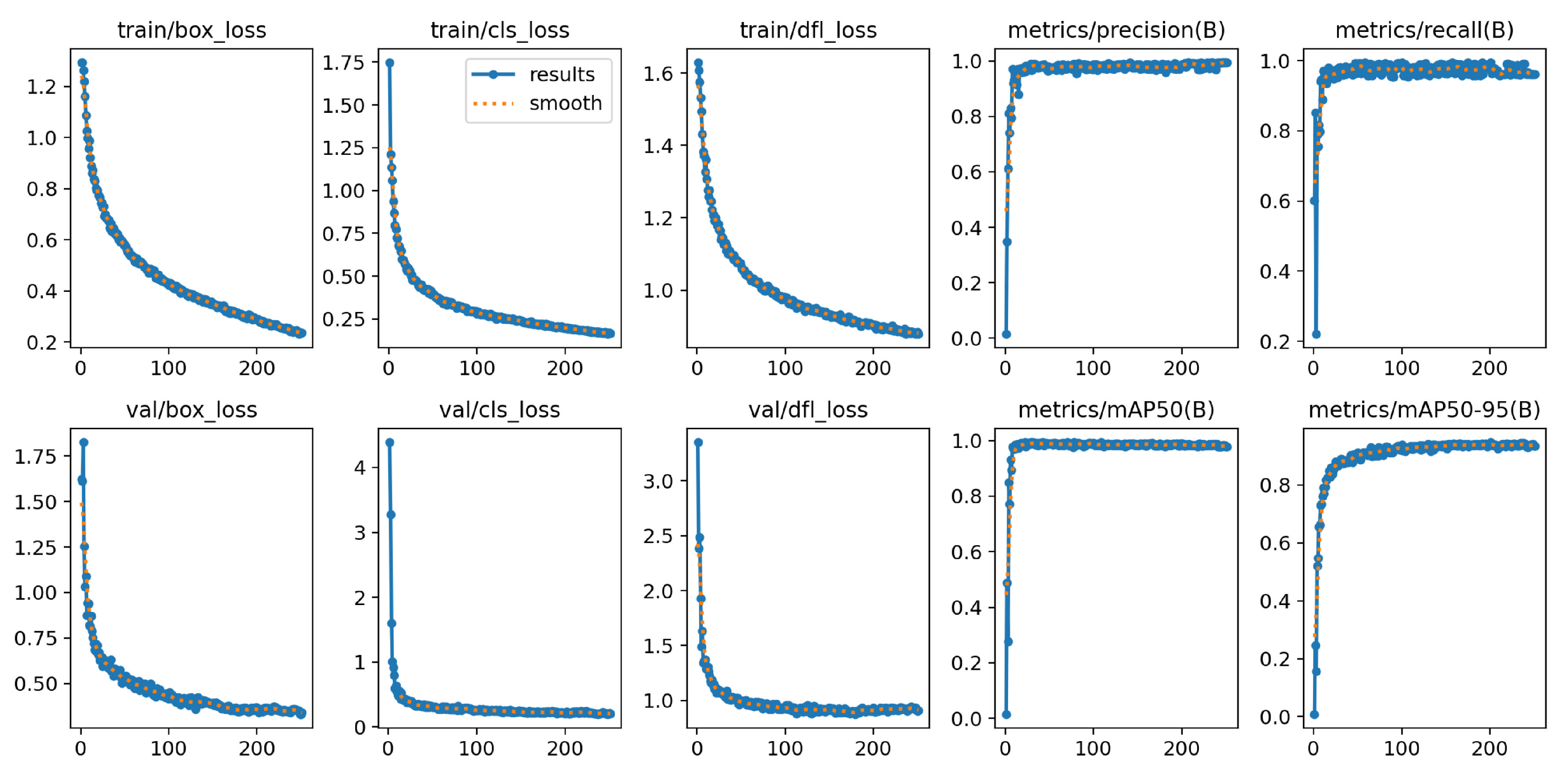
With 43.63 million parameters and 365 layers, the YOLOv8l-BV is the largest model architecture in this study. The training was stopped prematurely after 1:57 hours and ran over 251 epochs. The best model was selected in epoch 201 and has a size of 87.7 MB.
Figure 15 shows that the loss functions decrease continuously during training and converge to a minimum early on the validation dataset. The
graph converges to a maximum after a few epochs. The course of the
approaches the maximum exponentially.
3.2.2. Training Results Bird’s Eye and Side View
As the same YOLO models were used for datasets BV and BSV, the number of parameters, the layers and the model sizes do not differ. This enables a direct comparison of the results between the two datasets and makes it easier to analyse the performance of the YOLO models.
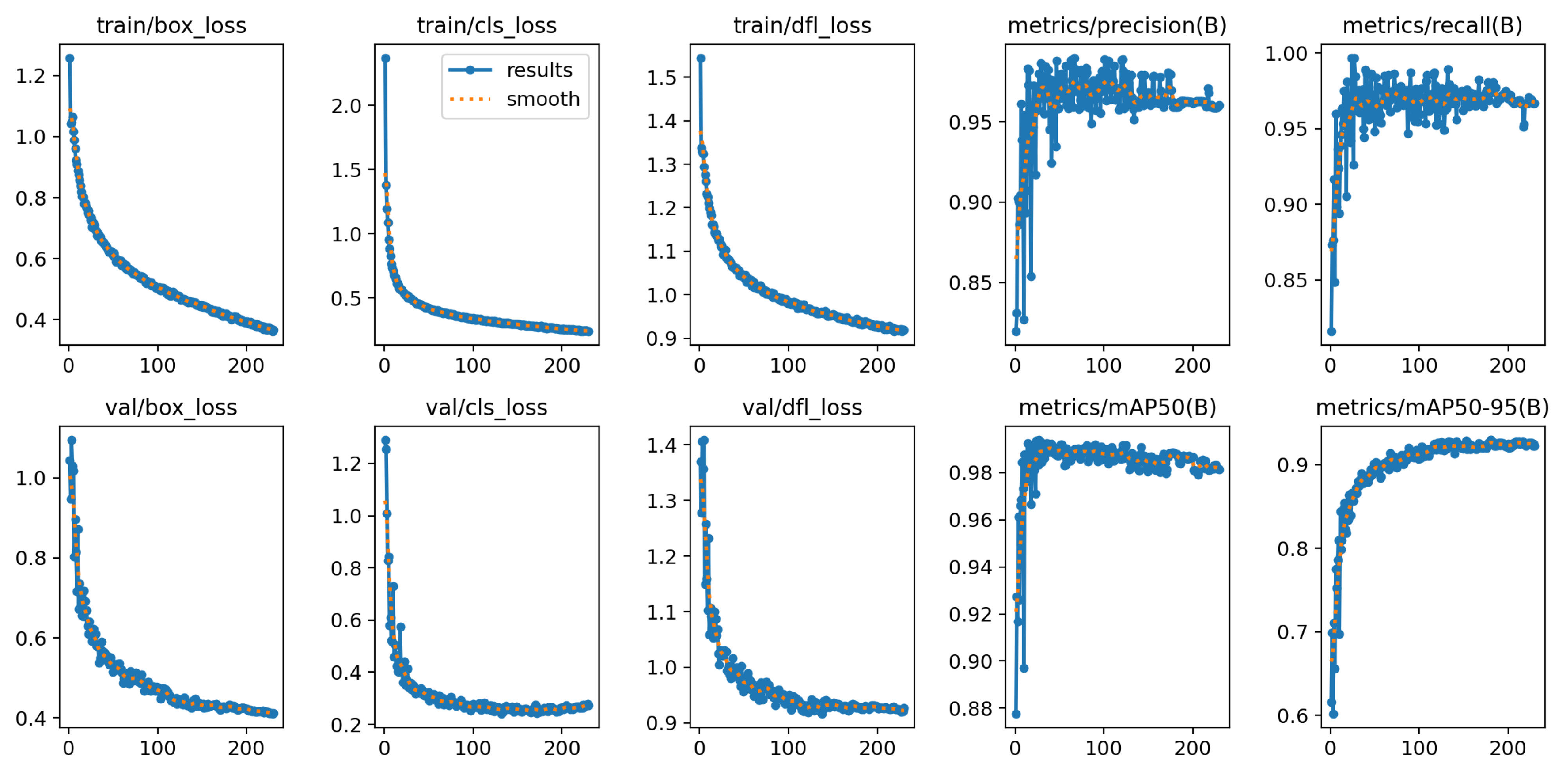
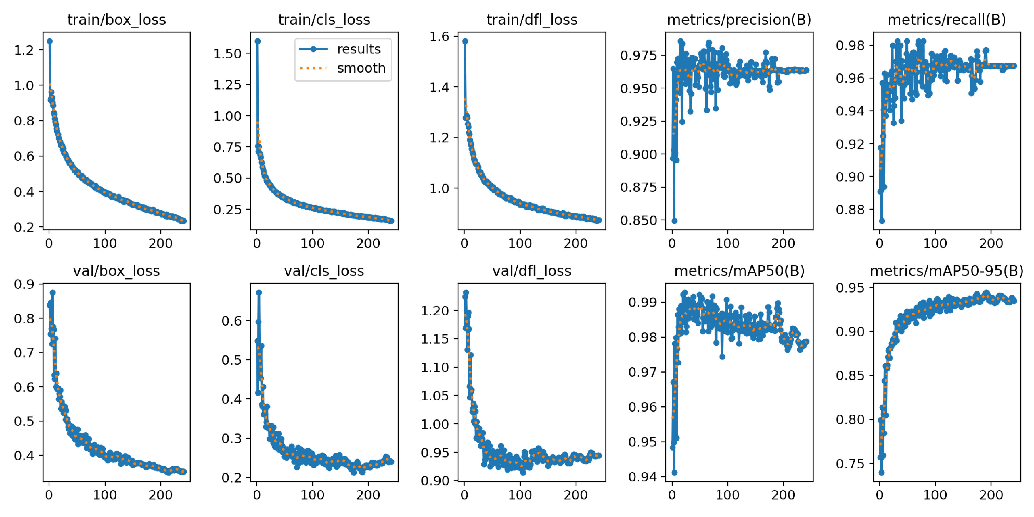
The loss functions of YOLOv8n-BSV during training, as can be seen on the first three graphs of
Figure 16, fall sharply monotonically at the beginning and then transition to a moderate drop after about 30 epochs. The loss functions of the validation converge after a rapid initial decrease. The
graph shows a minimal slope in the last 30 epochs. The training lasted 54 minutes and stopped early after 230 epochs, as the validation loss of the last 50 epochs did not change. The best results were observed in epoch 180. The graph of the
rises sharply at the beginning and flattens out slightly after reaching the maximum, which becomes apparent when the
y-axis is set precisely. The
resembles a logarithmic curve.
The
value is 98.8 % and is almost identical in the respective individual classes, with Flowering achieving the lowest value at 97.8 %. Growing has the lowest
value at 89.1 %. Flowering and Fruiting are almost identical at 95.1 % and 94.9 % and achieve a total of 93.0 %, as shown in
Table 9.
After 2 hours and 28 minutes, the training of YOLOv8m-BSV was finished early over 241 epochs. The best model was achieved in epoch 191. In
Figure 17, the training losses show strongly decreasing curves at the beginning and then approach a minimum. The validation losses
and
increase slightly towards the end of training. The
graph rises sharply and flattens out slightly, which becomes apparent with precise scale adjustment. The
graph also rises sharply at the beginning, but then slows down and converges in the last epochs.
The
value of the trained model on the validation data of the entire classes is 98.8 %. The
value is slightly lower at 94.4 %, as shown in
Table 10. Growing achieves the highest score of 99.4 % for the
and the lowest score of 91.6 % for the
. Flowering achieved the highest value for the
with 96.6 %.
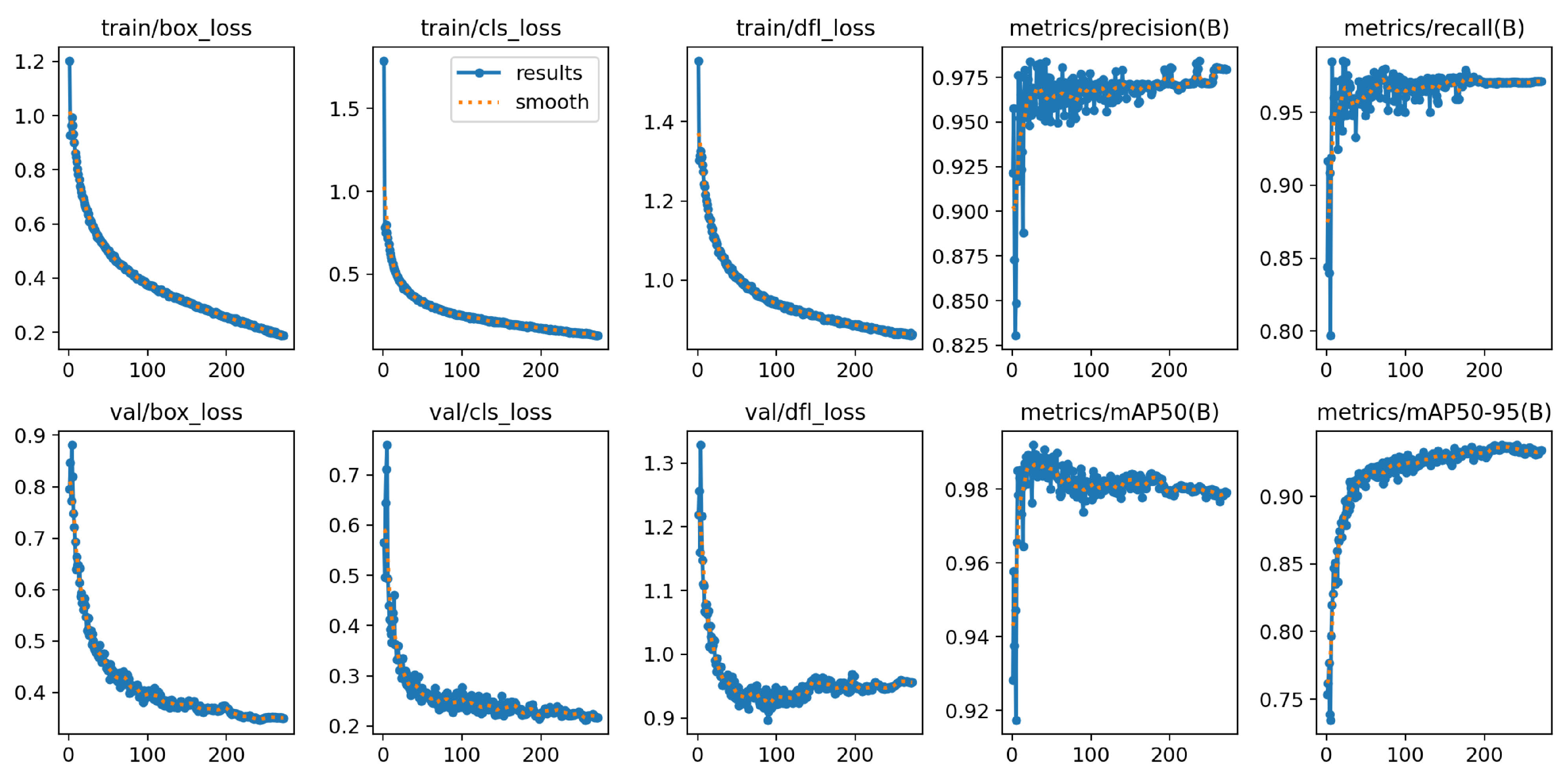
Figure 18 shows the training values of the YOLOv8l-BSV, which stopped prematurely after 272 of 300 epochs. The training thus lasted 4 hours and 8 minutes. The training loss graphs fall sharply at the beginning and then transition to a moderate decline. The validation losses also drop sharply at the beginning, slow down after about 50 epochs and then approach their minimum. A slight increase in
can be seen after 100 epochs. The
and
graphs behave in a similar way to YOLOv8n-BSV.
Table 11 illustrates the values achieved by YOLOv8l-BSV. The
value is 98.0 % and the
value is 93.8 %. An analysis of the individual classes shows that the Growing and Fruiting classes are almost the same for
. Only Flowering achieves a slightly lower value of 96.9 %. Growing achieves the lowest value with an
of 91.7 % and Flowering the highest at 95.8 %.
3.2.3. Summary of the Training Results
The performance of the proposed plant growth stage detection system using YOLOv8n-BV, YOLOv8m-BV and YOLOv8l-BV models was high. The loss functions of the three models indicate improved model learning, as the values of the training losses continuously decrease and those of the validation losses do not increase. This trend indicates that no overfitting has taken place. YOLOv8n-BV shows a sudden drop in training losses at the end of training. This behaviour can be interpreted in the context of the closure of the mosaic augmentation. In the last 10 epochs, the augmentation of the data is closed in order to avoid a deterioration of the training performance. The training losses of YOLOv8n-BSV, YOLOv8m-BSV and YOLOv8l-SBV decrease over all epochs. The validation losses for YOLOv8n-BSV and YOLOv8m-BSV and for YOLOv8m-BSV and YOLOv8l-BSV increase slightly, indicating the beginning of overfitting of the models.
Table 12 summarises the training results for all models. The models achieve similarly high
values, with YOLOv8n-BV and YOLOv8m-BV achieving the highest accuracies of 99.0 % each and YOLOv8l-BSV achieving the lowest value of 98.0 %. With dataset BV, YOLOv8l-BV achieves the highest value
with 94.8 %, while YOLOv8n-BSV achieves the lowest value of 93.0 % with dataset BSV. All models, except YOLOv8n-BV, stop training prematurely. YOLOv8m-BV is the first to stop the calculation after 197 epochs. With the BSV dataset, all models stop the training earlier.
The total training time for all models is 11 hours and 4 minutes. As expected, the small model YOLOv8n-BV with the smaller dataset BV has the shortest training time of 38 minutes. The YOLOv8l-BSV takes the longest to train at 4 hours and 8 minutes.
3.3. Test Results
Test dataset BV, consisting of 149 images and 242 labels, was used for all trained models. This ensures the comparability of all models. For the interpretation of the results, the of all classes is shown on the one hand and the confusion matrix is used on the other hand, as it provides a clear representation of the type of error. Precision and recall can be derived from this.
3.3.1. Test Results Bird’s Eye View
The
of YOLOv8n-BV, YOLOv8m-BV and YOLOv8l-BV are listed in
Table 13. It contains both the results of the individual classes and the overall values. YOLOv8l-BV achieves the highest
value across all classes on test dataset BV with 93.4 %. YOLOv8m-BV achieves the lowest value with 0.8 % less. YOLOv8n-BV achieves 92.9 % and lies between the MEDIUM and LARGE models. All three models achieve almost similar results for the Growing and Fruiting classes. YOLOv8l-BV achieves the highest values. The largest model also achieves the highest accuracy for the Flowering class with 96.1 %. In summary, YOLOv8l-BV has the highest
values overall in all classes, indicating precise object recognition and localisation, especially in the Flowering stage.
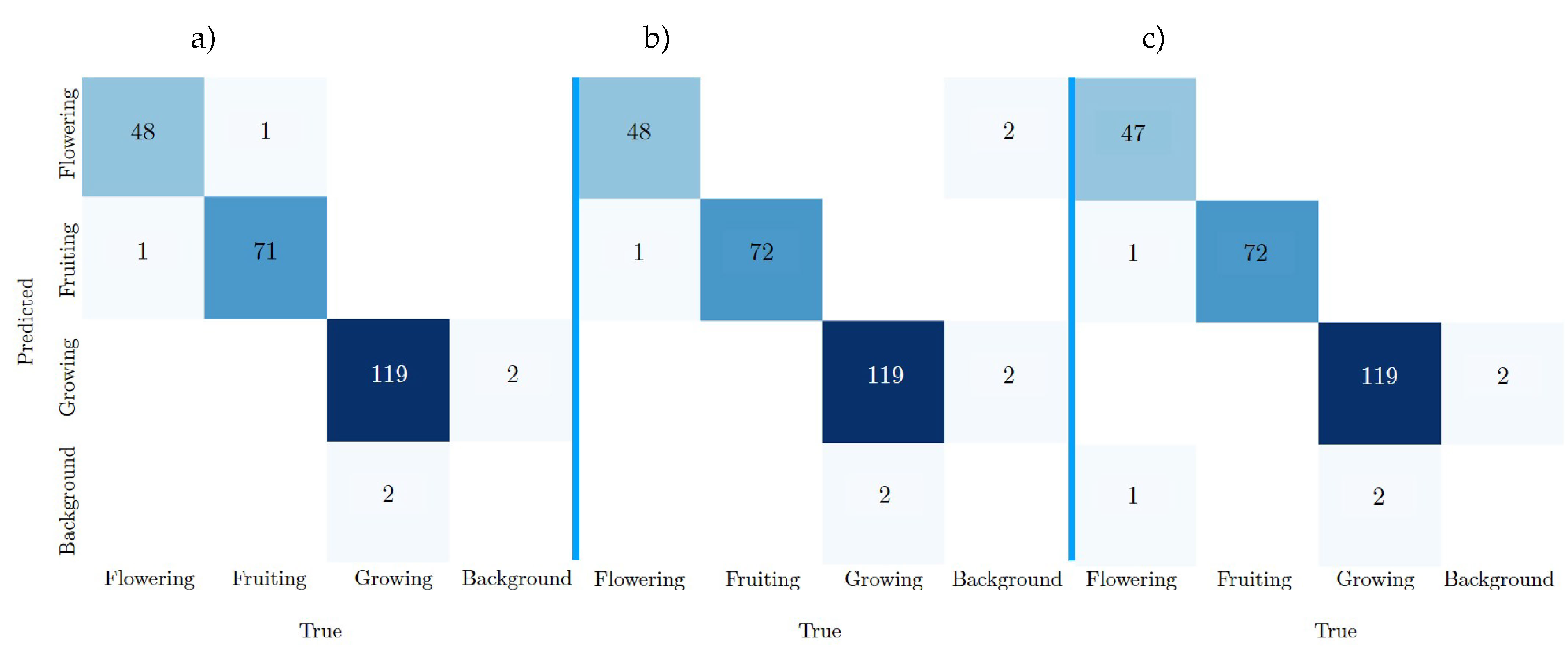
In the context of object recognition, the confusion matrix provides insight into the accuracy of predictions and the frequency of misclassifications. The "Background" class is an essential component of the YOLO algorithm and is automatically output, classifying regions without objects.
Figure 19 shows the confusion matrices of the YOLOv8n-BV, YOLOv8m-BV and YOLOv8l-BV test results. The true classes are shown in the columns, the predicted classes of the calculation are shown in the rows.
Table 2 (in
Section 2.3.3) shows that the test dataset BV contains 242 labels.
YOLOv8m-BV predicts 239 of the labels, which also correspond to the ground truth, as shown in the confusion matrix a). The model thus achieves the highest number of TP values. YOLOv8m-BV (see matrix b)) and YOLOv8l-BV (see matrix c)) follow with 238 TP each. YOLOv8m-BV (b) and YOLOv8l-BV (c) are error free in the Fruiting class, recognising all labels. All models predict Fruiting once, although it corresponds to the class Flowering (row 2, column 1). The same is true for two FNs in the Growing class, which are misinterpreted twice as Background (row 4, column 3). Each model predicts two labels in the Growing class, although it corresponds to the Background class (row 3, column 4). The YOLOv8m-BV achieves the most frequent FP with 4 errors, the YOLOv8l-BV the fewest with 2 errors.
3.3.2. Test Results Bird’s Eye and Side View
Table 14 shows the training results of the YOLOv8n-BSV, YOLOv8m-BSV and YOLOv8l-BSV on the test dataset BV. All models achieved high values on the test dataset. YOLOv8m-BSV achieved the highest
value of 96.3 % and YOLOv8l-BSV achieved the second highest value of 95.6 %, 0.7 % lower. YOLOv8m-BSV also achieves the highest accuracies in the individual Growing, Flowering and Fruiting classes. The YOLOv8n-BSV achieves the lowest overall result with 93.7 %. Looking at the individual classes, it can be seen that all models achieve particularly good results for the Flowering class, with values between 97.3 % and 98.8 %. The lowest scores were achieved by all models in the Growing class.
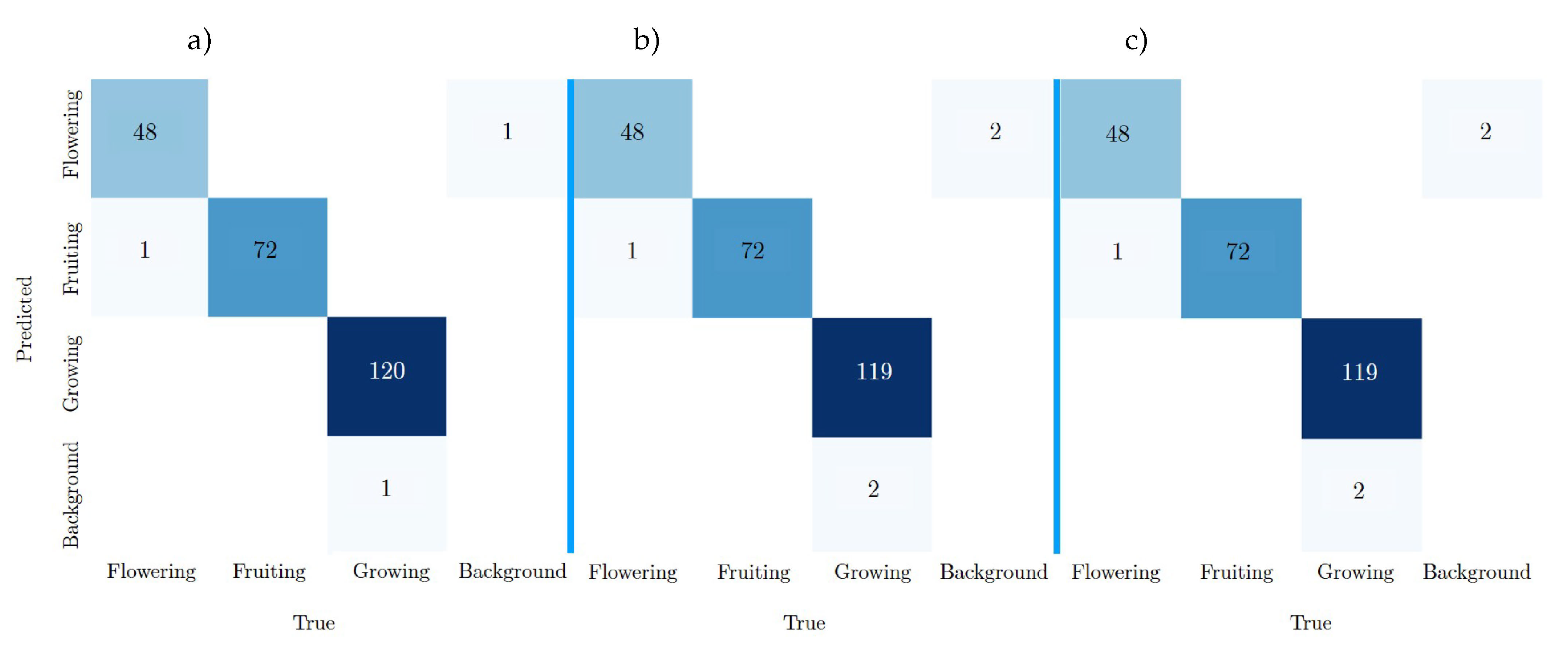
As can be seen in
Figure 20 of the confusion matrix a), YOLOv8n-BSV achieves the most TPs with 240 out of the 242 labels from the test dataset BV. This is followed by YOLOv8m-BSV and YOLOv8l-BSV with 239 true predictions each. YOLOv8m-BSV and YOLOv8l-BSV have exactly the same values. As the models in
Section 3.3.1 already show, all models predict Fruiting once, even though it corresponds to the Flowering class (row 2, column 1). YOLOv8n-BSV has the least FN and FP with two and one errors respectively.
3.3.3. Summary of the Test Results
Table 15 shows the
values achieved by all trained models on the test dataset BV. These are compared with the
values after training on the respective validation datasets. To illustrate the validation results by way of example,
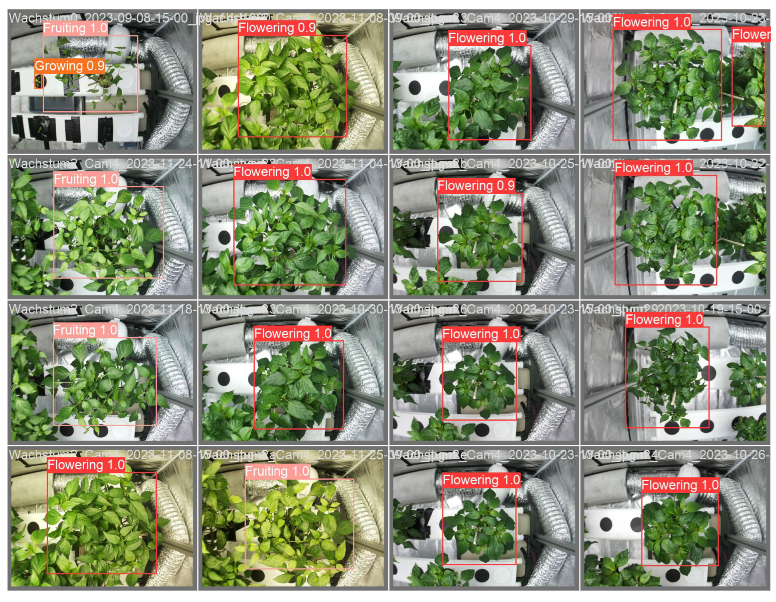
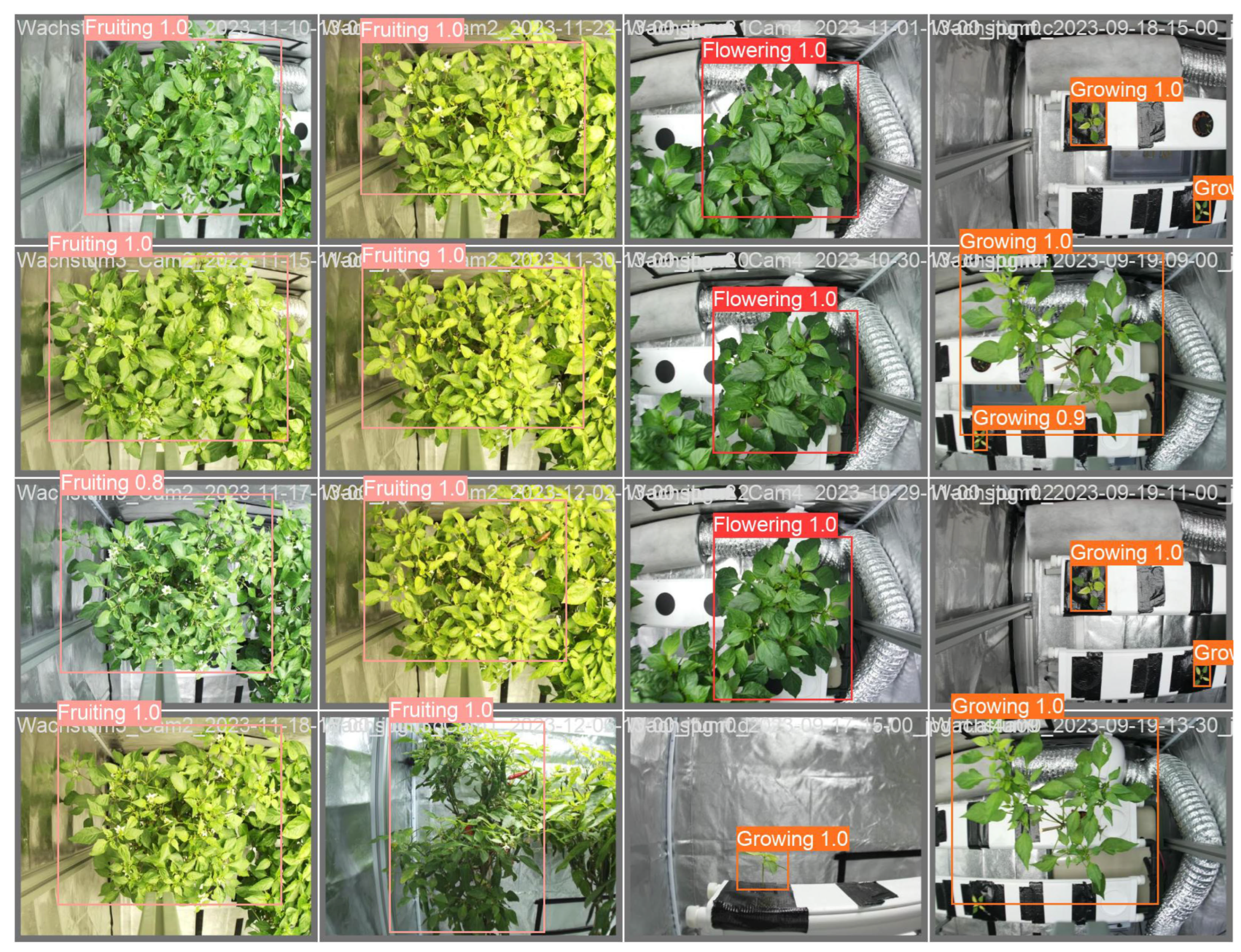
Figure 21 and
Figure 22 are shown.
Table 15.
Key performance figures of the tested YOLOv8 models with comparative values from training.
Table 15.
Key performance figures of the tested YOLOv8 models with comparative values from training.
| Model |
mAP50/% Test |
mAP50-95/% Validation |
Precision/% |
Recall/% |
| Bird’s eye view |
| YOLOv8n-BV |
92.9 |
94.4 |
98.8 |
98.8 |
| YOLOv8m-BV |
92.6 |
94.2 |
98.4 |
98.8 |
| YOLOv8l-BV |
93.4 |
94.8 |
99.2 |
98.4 |
| Bird’s eye and side view |
| YOLOv8n-BSV |
93.7 |
93.0 |
99.6 |
99.2 |
| YOLOv8m-BSV |
96.3 |
94.4 |
99.2 |
98.8 |
| YOLOv8l-BSV |
95.6 |
93.8 |
99.2 |
98.8 |
Overall, all models achieve a high value on the test dataset BV. YOLOv8m-BSV achieves the highest value on the test dataset with 96.3 %. With 3.7 % less, YOLOv8m-BV is the model with the lowest value at 92.6 %. Both models achieve values in the middle of the range on their respective validation datasets.
The precision and recall values are derived from TP, FN and FP. The values of all models are very close to each other. YOLOv8n-BSV achieves the highest precision and recall value with 99.6 % and 99.2 % of all models. The lowest precision value is achieved by YOLOv8m-BV with 98.4 % and the lowest recall value is achieved by YOLOv8l-BV, also with 98.4 %.
Figure 21.
Exemplary validation results using YOLOv8m for the growth stage detection from a bird’s eye view.
Figure 21.
Exemplary validation results using YOLOv8m for the growth stage detection from a bird’s eye view.
Figure 22.
Exemplary validation results using YOLOv8m for the growth stage detection from bird’s eye and side view.
Figure 22.
Exemplary validation results using YOLOv8m for the growth stage detection from bird’s eye and side view.
4. Discussion
4.1. Image Quality
The successful acquisition of data by the camera system over the entire survey period suggests that the chosen image resolution was sufficient to allow reliable identification of features such as buds, flowers, fruit set and fruit. This is confirmed by the results, as all trained models show an accuracy of over 98 % in identifying the classes.
The influence of image quality on model training, in terms of barrel distortion, yellowing and widened bounding boxes due to image rotation, cannot be determined from the results presented. Further research is required to gain a full understanding of the impact of these image quality factors.
4.2. Data and Model Discussion
The results show that all models are able to identify the three growth stages of the plants. They achieved an accuracy of at least 92.6 % on the test dataset BV with respect to the metric .
The best training results were achieved by the YOLO models trained only on the bird’s eye view dataset. This does not confirm the assumption that extending the dataset to include the side view improves training performance. YOLOv8l-BV achieved the highest training values with 94.8 % , which supports the assumption that larger models achieve better accuracies. The smallest YOLOv8n-BV is just behind with 94.4 %. In addition, the model did not converge after 300 epochs. In contrast to YOLOv8l-BV, YOLOv8n-BV shows the potential for improvement by increasing the number of epochs. With regard to the training evaluation, the assumption of higher accuracy with large models cannot be confirmed and requires further investigation.
The test results paint a mixed picture of accuracy depending on model size and data influence. On average, YOLOv8n-BV, YOLOv8m-BV and YOLO-V8l-BV have lower accuracies than YOLOv8n-BSV, YOLOv8m-BSV and YOLOv8l-BSV. This indicates that models trained on the extended dataset BSV show better generalisation. Of all the models, the medium model (YOLOv8m-BSV) trained on the BSV dataset performed best, followed by the two large models YOLOv8l-BSV and YOLOv8l-BV. This suggests that larger models tend to perform better, although this assumption cannot be conclusively confirmed as the medium model (YOLOv8m-BSV) performed best in this particular application.
Looking at the individual classes in more detail, it is noticeable that all models achieved the lowest
values in the Growing class, even though this class had the most labels (see
Table 2). This observation may be due to the quality of the dataset. It is possible that the recording of four images per day and additional augmentation resulted in some redundancy in the data. This may lead to overfitting of the class during training and affect the ability of the models to generalise to previously unseen data.
The precision and recall values of all models on the test dataset BV are very close to each other at a high level. Precision plays a crucial role in this study, as accurate prediction of classes or growth stages should ensure that future environmental conditions for plant growth are optimised. The smallest model with the BSV dataset (YOLOv8n-BSV) gave the best results. However, due to the small differences between the values, no general statement can be made about the effect of data sets and model sizes on accuracy.
In particular, the evaluation of the test results showed incorrect predictions corresponding to the Background class. These errors could be due to the lack of Background images in the dataset. In order to minimise these FP errors and improve the generalisability of the model, it would be advisable to include a dataset with background images in the next calculations. In particular, these should include images of the growth box and future application areas.
It is important to emphasise that the models developed and the results obtained in this work are only valid for the specific use case with the considered plants in the defined grow box environment. The future challenge is to ensure that the developed models can prove their performance in different scenarios and that their robustness and applicability are validated in a broader context.
5. Conclusion and Future Directions
In this work, images of chilli plants of the species Capsicum annuum, grown in a hydroponic environment, were taken from two views over their life cycle, from seedling to fruit. The bird’s eye and side view data were collected over a period of four months and used to train the models. The three models YOLOv8n, YOLOv8m and YOLOv8l were trained using data sets BV and BSV. This resulted in the six models YOLO-V8n-BV, YOLO-V8m-BV, YOLO-V8l-BV, YOLO-V8n-BSV, YOLO-V8m-BSV and YOLO-V8l-BSV.
All six models are able to recognise the growth stages of chilli plants from a bird’s eye view. The high accuracy of the models confirms the objective. The HQ Raspberry Pi camera with a 6mm wide angle lens provided images of sufficient quality to train the YOLO models.
The test results of all models show a comparably high level. Overall, the BSV dataset showed the best results in terms of and precision. The influence of the model size is not clear, as the medium architecture of YOLO gave the best results.
In order to improve the models in the future, the influence of image quality can be analysed. The short distance between the lens and the plants has led to distortion of the images. In addition, part of the dataset has a yellowish tinge. These images can be corrected using image processing algorithms. It is necessary to check whether the corrected images have any effect on the calculation results. In general, these phenomena can be avoided by using appropriate software and high quality hardware. In addition, the dataset should be checked for redundant or inconspicuous features and compared with the results obtained.
Further optimisation could be achieved by hyperparameter tuning. By increasing the number of epochs, the YOLOv8- BV could achieve better results. In addition, the image resolution (image size) can be increased and a k-fold cross-validation can be performed. Expanding the dataset to include background images can also lead to improvements and can be compared with the results obtained in this work.
The next step is to test the generalisability of the model on unknown data. This can be done by compiling a common set of data and evaluating the accuracy of the predictions. The reliability of the system can also be tested by growing new chilli plants. The newly generated images can directly contribute to the improvement of the system by increasing the diversity of the dataset.
In this work, the plant in the images was considered as a whole and fed into the model training. Further research can create a dataset with specific annotations of the buds, flowers and fruits and compare the training results.
The trained models can be used as a holistic image processing system for targeted and intelligent control of the next cultivation process. Depending on the predictions, growth parameters such as light and nutrient composition can be adjusted. The main objectives of the study are energy consumption and yield, which will be compared with cultivation without an image processing system.
Another option for analysing the models is the need for computing power. Can edge computing, such as Raspberry Pi or Raspberry Pi Zero W, be used, or will centralised computing, such as cloud computing, be required? As larger models require more computing resources, the processing speed or inference time of the models needs to be evaluated as a function of performance. These devices could be used in a mobile design in greenhouses or vertical indoor farms.
Other applications of machine vision in hydroponics include disease and nutrient deficiency detection, as well as flower and fruit detection for pollination and targeted harvesting. The YOLO models created can be used as pre-trained models and as a starting point for the development of new computations in these application areas.
Abbreviations
The following abbreviations are used in this manuscript:
| AP |
Average Precision |
| BV |
Bird’s Eye View |
| BSV |
Bird’s Eye and Side View |
| CAISA |
Cologne Lab for Artificial Intelligence and Smart Automation |
| cls loss |
class loss |
| CNN |
Convolutional Neural Network |
| CPU |
Central Processing Unit |
| dfl loss |
defocus loss |
| DL |
Deep Learning |
| EC |
Electric Conductivity |
| FN |
False Negative |
| FP |
False Positive |
| GB |
Gigabyte |
| GPU |
Graphical Processing Unit |
| IDE |
Integrated Development Environment |
| IoU |
Intersection over Union |
| LED |
Light-Emitting Diode |
| mAP |
mean Average Precision |
| MB |
Megabyte |
| ML |
Machine Learning |
| MV |
Machine Vision |
| NFT |
Nutrient Film Technique |
| PAR |
Photosynthetically Active Radiation |
| pH |
potential Hydrogen |
| PPFD |
Photosynthetically Active Photon Flux Density |
| PR |
Precision-Recall |
| SV |
Side View |
| TN |
True Negative |
| TP |
True Positive |
| VIF |
Vertical Indoor-Farming / Vertical Indoor-Farm |
| YOLO |
You Only Look Once |
References
- Despommier, D. D. The Vertical Farm: Feeding the World in the 21st Century; Picador: USA, 2020.
- Polsfuss, L. PFLANZEN. Available online: https://pflanzenfabrik.de/hydroponik/pflanzen/ (accessed on 5 April 2024).
- Available online: https://chili-plants.com/chilisorten/ (accessed on 2 December 2023).
- Drache, P. Chili Geschichte, Herkunft und Verbreitung. Available online: https://chilipflanzen.com/wissenswertes/chili-geschichte/ (accessed on 2 December 2023).
- Azlan, A.; Sultana, S.; Huei, C. S.; Razman, M. R. Antioxidant, Anti-Obesity, Nutritional and Other Beneficial Effects of Different Chili Pepper: A Review. Molecules 2022, 27, 898. https://www.mdpi.com/1420-3049/27/3/898.
- Thiele, R. Untersuchungen zur Biosynthese von Capsaicinoiden – Vorkommen und Einfluss von Acyl-Thioestern auf das Fettsäuremuster der Vanillylamide in Capsicum spp.; Dissertation, Bergische Universität Wuppertal, 2008. Available online: https://elekpub.bib.uni-wuppertal.de/urn/urn:nbn:de:hbz:468-20080466.
- Meier, U. Entwicklungsstadien mono- und dikotyler Pflanzen: BBCH Monografie, Quedlinburg, 2018. https://www.openagrar.de/receive/openagrar_mods_00042352.
- Feldmann, F.; Rutikanga, A. Phenological growth stages and BBCHidentification keys of Chilli (Capsicum annuum L., Capsicum chinense JACQ., Capsicum baccatum L. J. Plant Dis. Prot. 2021, 128, 549–555. [CrossRef]
- Paul, N. C.; Deng, J. X.; Sang, H.-K.; Choi, Y.-P.; Yu, S.-H. Distribution and Antifungal Activity of Endophytic Fungi in Different Growth Stages of Chili Pepper (Capsicum annuum L.) in Korea. The Plant Pathology Journal 2012, 28, 10–19. [CrossRef]
- Paul, A.; Nagar, H.; Machavaram R. Utilizing Fine-Tuned YOLOv8 Deep Learning Model for Greenhouse Capsicum Detection and Growth Stage Determination. In Proceedings of the 2023 7th International Conference on I-SMAC (IoT in Social, Mobile, Analytics and Cloud), Kirtipur, Nepal: IEEE, 11–13 Oct. 2023; pp. 649–656. https://ieeexplore.ieee.org/document/10290335.
- Kamilaris, A. Prenafeta-Boldú, F. X. A review of the use of convolutional neural networks in agriculture. J. Agric. Sci. 2018, 156, 312–322. [CrossRef]
- Tian, H.; Wang, Liu, Y.; Qiao, X.; Li, Y. Computer vision technology in agricultural automation —A review. Information Processing in Agriculture 2020, 7, 1–19. [CrossRef]
- Lin, K.; Chen, J.; Si, H.; Wu, J. A Review on Computer Vision Technologies Applied in Greenhouse Plant Stress Detection. In: Tan, T.; Ruan, Q.; Chen, X.; Ma, H.; Wang, L. (eds) Advances in Image and Graphics Technologies. IGTA 2013. Communications in Computer and Information Science, 363, Berlin: Springer. [CrossRef]
- Wijanarko, A.; Nugroho, A. P.; Kusumastuti, A. I.; Dzaky, M. A. F.; Masithoh, R. E.; Sutiarso, L.; Okayasu, T. Mobile mecavision: automatic plant monitoring system as a precision agriculture solution in plant factories. IOP Conf. Series: Earth and Environmental Science 2021, 733, 012026. https://iopscience.iop.org/article/10.1088/1755-1315/733/1/012026.
- Samiei, S.; Rasti, P.; Ly Vu, J.; Buitink, J.; Rousseau, D. Deep learning-based detection of seedling development. Plant Methods 2020, 16, 103. [CrossRef]
- Yeh, Y.-H. F. ; Lai, T.-C.; Liu, T.-Y.; Liu, C.-C.; Chung, W.-C.; Lin, T.-T. An automated growth measurement system for leafy vegetables. Biosystems Engineering 2014, 117, 43–50. [CrossRef]
- Nugroho, A. P.; Fadilah, M. A. N.; Wiratmoko, A.; Azis, Y. A.; Efendi, A. W.; Sutiarso, L.; Okayasu, T. Implementation of crop growth monitoring system based on depth perception using stereo camera in plant factory. IOP Conf. Series: Earth and Environmental Science 2020, 542, 012068. https://iopscience.iop.org/article/10.1088/1755-1315/542/1/012068.
- Available online: https://www.pflanzenforschung.de/de/pflanzenwissen/lexikon-a-z/phaenotypisierung-10020 (accessed on 2 December 2023).
- Li, Z.; Guo, R.; Li, M.; Chen, Y.; Li, G. A review of computer vision technologies for plant phenotyping. Computers and Electronics in Agriculture 2020, 176, 105672. [CrossRef]
- Redmon, J.; Divvala, S. K.; Girshick, R. B.; Farhadi, A. You Only Look Once: Unified, Real-Time Object Detection. In Proceedings of the 2016 IEEE Conference on Computer Vision and Pattern Recognition (CVPR), Las Vegas, NV, USA, 27–30 June 2016, pp. 779–788. https://ieeexplore.ieee.org/document/7780460.
- Hespeler, S. C.; Nemati, H.; Dehghan-Niri, E. Non-destructive thermal imaging for object detection via advanced deep learning for robotic inspection and harvesting of chili peppers. Artificial Intelligence in Agriculture 2021, 5, 102–117. [CrossRef]
- Coleman, G. R.; Kutugata, M.; Walsh, M. J.; Bagavathiannan, M. Multi-growth stage plant recognition: a case study of Palmer amaranth (Amaranthus palmeri) in cotton (Gossypium hirsutum). arXiv 2023, arXiv:2307.15816. https://arxiv.org/abs/2307.15816.
- Zhang, P.; Li, D. CBAM + ASFF-YOLOXs: An improved YOLOXs for guiding agronomic operation based on the identification of key growth stages of lettuce. Computers and Electronics in Agriculture 2022, 203, 107491. [CrossRef]
- grow-shop24. DiamondBox Silver Line SL150, 150×150×200cm. Available online: https:// www.grow-shop24.de/diamondbox-silver-line-sl150 (accessed on 8 June 2023).
- Available online: https://docs.roboflow.com/ (accessed on 6 December 2023).
- Buslaev, A.; Iglovikov, V. I.; Khvedchenya, E.; Parinov, A.; Druzhinin, M.; Kalinin, A. A. Albumentations: Fast and Flexible Image Augmentations. Information 2020, 11, 125. https://www.mdpi.com/2078-2489/11/2/125.
- Jocher, G.; Chaurasia, A.; Qiu, J. YOLO by Ultralytics. Available online: https://github.com/ultralytics/ultralytics (accessed on 30 November 2023).
- Lou, H.; Duan, X.; Guo, J.; Liu, H.; Gu, J.; Bi, L.; Chen, H. DC-YOLOv8: Small-Size Object Detection Algorithm Based on Camera Sensor. Electronics 2023, 12, 2323. [CrossRef]
- Pan, Y.; Xiao, X.; Hu, K.; Kang, H.; Jin, Y.; Chen, Y.; Zou, X. ODN-Pro: An Improved Model Based on YOLOv8 for Enhanced Instance Detection in Orchard Point Clouds. Agronomy 2024, 14, 697. [CrossRef]
- Liu, S.; Qi, L.; Qin, H.; Shi, J.; Jia, J. Path Aggregation Network for Instance Segmentation. In Proceedings of the IEEE Conference on Computer Vision and Pattern Recognition, Salt Lake City, UT, USA, 18–23 June 2018; pp. 8759–8768. https://ieeexplore.ieee.org/document/8579011.
- Lin, T.; Girshick, R.; He, K.; Hariharan, B.; Belongie, S. Feature Pyramid Networks for Object Detection. In Proceedings of the IEEE Conference on Computer Vision and Pattern Recognition, Honolulu, Hawaii, USA, 21–26 July 2017; pp. 2117–2125. https://ieeexplore.ieee.org/document/8099589.
- Lin, T.Y.; Maire, M.; Belongie, S.; Hays, J.; Perona, P.; Ramanan, D.; Dollár, P.; Zitnick, C.L. Microsoft COCO: Common Objects in Context; Springer: Berlin/Heidelberg, Germany, 2014; Volume 8693, pp. 740–755. https://link.springer.com/chapter/10.1007/978-3-319-10602-1_48.
- Padilla, R.; Passos,W. L.; Dias, T. L. B.; Netto, S. L., da Silva, E. A. B. A Comparative Analysis of Object Detection Metrics with a Companion Open-Source Toolkit. Electronics 2021, 10, 279. [CrossRef]
- Akbarnezhad, E. YOLOv8 Projects #1 "Metrics, Loss Functions, Data Formats, and Beyond". Available online: https://www.linkedin.com/pulse/yolov8-projects-1-metrics-loss-functions-data-formats-akbarnezhad/ (accessed on 16 November 2023).
Figure 1.
Structure of the machine vision system from image acquisition, image pre-processing to modeling process (computer vision).
Figure 1.
Structure of the machine vision system from image acquisition, image pre-processing to modeling process (computer vision).
Figure 2.
(Experimental setup for image generation with the camera systems outlined in blue.
Figure 2.
(Experimental setup for image generation with the camera systems outlined in blue.
Figure 3.
(a) Experimental set-up with dimensions labelled in black/bold for the growth stage Growing and in blue/bold for the stages Flowering and Fruiting; (b) Mounted camera systems for the side view (left) and the bird’s eye view (right).
Figure 3.
(a) Experimental set-up with dimensions labelled in black/bold for the growth stage Growing and in blue/bold for the stages Flowering and Fruiting; (b) Mounted camera systems for the side view (left) and the bird’s eye view (right).
Figure 4.
The same picture after applying the transformations three times with bounding box.
Figure 4.
The same picture after applying the transformations three times with bounding box.
Figure 5.
Data distribution of the labels according to the classes Growing, Flowering and Fruiting for (a) the bird’s eye view; (b) the bird’s eye and side view.
Figure 5.
Data distribution of the labels according to the classes Growing, Flowering and Fruiting for (a) the bird’s eye view; (b) the bird’s eye and side view.
Figure 6.
Training flow of the developed growth stage detection procedure.
Figure 6.
Training flow of the developed growth stage detection procedure.
Figure 9.
Images of the 3 growth stages from a bird’s eye view.
Figure 9.
Images of the 3 growth stages from a bird’s eye view.
Figure 10.
Left image with and right image without yellow tint.
Figure 10.
Left image with and right image without yellow tint.
Figure 11.
Image distortion with straight blue bar.
Figure 11.
Image distortion with straight blue bar.
Figure 12.
Bounding box after rotation of the image.
Figure 12.
Bounding box after rotation of the image.
Figure 13.
Loss functions and values after 300 epochs of the YOLOv8n-BV model with the dataset BV.
Figure 13.
Loss functions and values after 300 epochs of the YOLOv8n-BV model with the dataset BV.
Figure 14.
Loss functions and values after 300 epochs of the YOLOv8m-BV model with the dataset BV.
Figure 14.
Loss functions and values after 300 epochs of the YOLOv8m-BV model with the dataset BV.
Figure 15.
Loss functions and values after 300 epochs of the YOLOv8l-BV model with the dataset BV.
Figure 15.
Loss functions and values after 300 epochs of the YOLOv8l-BV model with the dataset BV.
Figure 16.
Loss functions and values after 300 epochs of the YOLOv8n-BSV model with the dataset BSV.
Figure 16.
Loss functions and values after 300 epochs of the YOLOv8n-BSV model with the dataset BSV.
Figure 17.
Loss functions and values after 300 epochs of the YOLOv8m-BSV model with the dataset BSV.
Figure 17.
Loss functions and values after 300 epochs of the YOLOv8m-BSV model with the dataset BSV.
Figure 18.
Loss functions and values after 300 epochs of the YOLOv8l-BSV model with the dataset BSV.
Figure 18.
Loss functions and values after 300 epochs of the YOLOv8l-BSV model with the dataset BSV.
Figure 19.
Confusion matrices of the test results for the daset BV: (a) YOLOv8n; (b) YOLOv8m; (c) YOLOv8l.
Figure 19.
Confusion matrices of the test results for the daset BV: (a) YOLOv8n; (b) YOLOv8m; (c) YOLOv8l.
Figure 20.
Confusion matrices of the test results for the daset BSV: (a) YOLOv8n; (b) YOLOv8m; (c) YOLOv8l.
Figure 20.
Confusion matrices of the test results for the daset BSV: (a) YOLOv8n; (b) YOLOv8m; (c) YOLOv8l.
Table 1.
Components of the camera system used in this study.
Table 1.
Components of the camera system used in this study.
| Item |
Quantity |
Item description |
| 1 |
4 |
HQ Raspberry Pi camera |
| 2 |
4 |
6MM WW Raspberry Pi lens |
| 3 |
4 |
Raspberry Pi Zero W |
| 4 |
1 |
Raspberry Pi 4 B |
| 5 |
2 |
Mantona 17996 travel tripod |
| 6 |
4 |
USB-A to USB-B-Mini 3 m cable |
| 7 |
1 |
USB-C power adapter |
| 8 |
5 |
Memory card SanDisk Ultra microSDHC 32GB |
| 9 |
1 |
Energenie Uni-4-fold USB charger |
Table 2.
Listing of labels by class and view.
Table 2.
Listing of labels by class and view.
| |
Bird’s eye view |
Bird’s eye and side view |
| |
Train (BV) |
Val (BV) |
Test B(V) |
Train (BSV) |
Val (BSV) |
Test (BSV) |
| Growing |
446 |
77 |
121 |
2,112 |
107 |
121 |
| Flowering |
498 |
28 |
49 |
914 |
39 |
49 |
| Fruiting |
624 |
26 |
72 |
1,932 |
95 |
72 |
Table 4.
Calculation setup.
Table 4.
Calculation setup.
| Data |
Values |
| CPU |
12th Gen Intel Core i9-13900 |
| RAM |
64 GB DDR5 |
| GPU |
NVIDIA RTX A5000 |
| Algorithm |
YOLOv8n, -v8m, -v8l |
Table 5.
Assignment of recognised bounding boxes with explanation.
Table 5.
Assignment of recognised bounding boxes with explanation.
| Assignement |
Explanation |
| True Positive (TP) |
Bounding box in the correct position (positive) and correct prediction (true) |
| False Positive (FP) |
Bounding box in the right place (positive), but wrong prediction (false) |
| False Negative (FN) |
Bounding box not recognised (negative) and incorrect prediction (false) |
| True Negative (TN) |
Bounding box not recognised (negative) and correct prediction (true); no influence for multiclass tasks |
Table 6.
mAP values of the YOLOv8n-BV model on the validation set V.
Table 6.
mAP values of the YOLOv8n-BV model on the validation set V.
| Classes |
mAP50 / % |
mAP50-95 / % |
| All |
99.0 |
94.4 |
| Growing |
98.3 |
90.1 |
| Flowering |
99.3 |
96.6 |
| Fruiting |
99.5 |
96.5 |
Table 7.
values of the YOLOv8m-BV model on the validation set V.
Table 7.
values of the YOLOv8m-BV model on the validation set V.
| Classes |
mAP50 / % |
mAP50-95 / % |
| All |
99.0 |
94.2 |
| Growing |
98.0 |
89.9 |
| Flowering |
99.4 |
95.9 |
| Fruiting |
99.5 |
97.0 |
Table 8.
values of the YOLOv8l-BV model on the validation set V.
Table 8.
values of the YOLOv8l-BV model on the validation set V.
| Classes |
mAP50 / % |
mAP50-95 / % |
| All |
98.9 |
94.8 |
| Growing |
97.8 |
91.0 |
| Flowering |
99.5 |
95.8 |
| Fruiting |
99.5 |
97.6 |
Table 9.
values of the YOLOv8n-BSV model on the validation set BSV.
Table 9.
values of the YOLOv8n-BSV model on the validation set BSV.
| Classes |
mAP50 / % |
mAP50-95 / % |
| All |
98.8 |
93.0 |
| Growing |
99.4 |
89.1 |
| Flowering |
97.8 |
95.1 |
| Fruiting |
99.3 |
94.9 |
Table 10.
values of the YOLOv8m-BSV model on the validation set BSV.
Table 10.
values of the YOLOv8m-BSV model on the validation set BSV.
| Classes |
mAP50 / % |
mAP50-95 / % |
| All |
98.8 |
94.4 |
| Growing |
99.4 |
91.6 |
| Flowering |
97.8 |
96.6 |
| Fruiting |
99.2 |
95.2 |
Table 11.
values of the YOLOv8l-BSV model on the validation set BSV.
Table 11.
values of the YOLOv8l-BSV model on the validation set BSV.
| Classes |
mAP50 / % |
mAP50-95 / % |
| All |
98.0 |
93.8 |
| Growing |
98.5 |
91.7 |
| Flowering |
96.9 |
95.8 |
| Fruiting |
98.7 |
94.0 |
Table 12.
Key performance indicators of the trained YOLOv8 models.
Table 12.
Key performance indicators of the trained YOLOv8 models.
| Model |
mAP50/% |
mAP50-95/% |
Epochs |
Training time/h |
Model size/MB |
| Bird’s eye view |
| YOLOv8n-BV |
99.0 |
94.4 |
300 |
0.576 |
6.3 |
| YOLOv8m-BV |
99.0 |
94.2 |
197 |
1.032 |
52 |
| YOLOv8l-BV |
98.9 |
94.8 |
251 |
1.956 |
87.7 |
| Bird’s eye and side view |
| YOLOv8n-BSV |
98.8 |
93.0 |
230 |
0.895 |
6.3 |
| YOLOv8m-SBV |
98.8 |
94.4 |
241 |
2.474 |
52 |
| YOLOv8l-BSV |
98.0 |
93.8 |
272 |
4.138 |
87.7 |
Table 13.
values of YOLOv8n-BV, YOLOv8m-BV and YOLOv8l-BV on the training dataset BV.
Table 13.
values of YOLOv8n-BV, YOLOv8m-BV and YOLOv8l-BV on the training dataset BV.
| |
YOLOv8n-BV |
YOLOv8m-BV |
YOLOv8l-BV |
| |
/% |
| All |
92.9 |
92.6 |
93.4 |
| Growing |
91.2 |
91.2 |
92.1 |
| Flowering |
95.6 |
95.4 |
96.1 |
| Fruiting |
91.9 |
91.1 |
91.9 |
Table 14.
values of YOLOv8n-BSV, YOLOv8m-BSV and YOLO-v8l-BSV on the training dataset BSV.
Table 14.
values of YOLOv8n-BSV, YOLOv8m-BSV and YOLO-v8l-BSV on the training dataset BSV.
| |
YOLOv8n-BSV |
YOLOv8m-BSV |
YOLOv8l-BSV |
| |
/% |
| All |
93.7 |
96.3 |
95.6 |
| Growing |
91.8 |
94.5 |
94.4 |
| Flowering |
97.3 |
98.8 |
98.3 |
| Fruiting |
92.0 |
95.7 |
94.2 |
|
Disclaimer/Publisher’s Note: The statements, opinions and data contained in all publications are solely those of the individual author(s) and contributor(s) and not of MDPI and/or the editor(s). MDPI and/or the editor(s) disclaim responsibility for any injury to people or property resulting from any ideas, methods, instructions or products referred to in the content. |
© 2024 by the authors. Licensee MDPI, Basel, Switzerland. This article is an open access article distributed under the terms and conditions of the Creative Commons Attribution (CC BY) license (http://creativecommons.org/licenses/by/4.0/).
