1. Introduction
Corrosion can weaken the structural integrity of a vessel, increasing the risk of catastrophic failure, such as hull breaches or structural collapses, and may lead to loss of life, environmental damage, and costly repairs. Operators can continuously improve corrosion management practices by close periodic monitoring of corrosion trends and identifying patterns, which allows for longitudinal evaluation of the effectiveness of mitigation measures. Inasmuch, inspectors pinpoint areas of accelerated deterioration, allowing for targeted inspections and preventive measures. This helps optimize maintenance efforts and ensures that critical components receive adequate attention.
In addition, assuming protective coatings have been used used, marine vessels must complete an inspection of the hull in a dry dock at least three times in a five-year period, with intermediate surveys being performed within 36 months. This relates to visual hull inspection requirements due to the Convention for Safety of Life At Sea (SOLAS) [
1]. The automation of such a laborious visual task would produce massive savings both in terms of person hours, as well as time required for a vessel to not being operational.
The problem of corrosion visual surveying (RGB images) by human inspectors and its automation, can be seen as an extension of semantic segmentation in images; i.e. the association of pixels to a specific class / label (corrosion) [
2,
3,
4]. Corrosion as isolated area units on a vessel surface is difficult to both detect and predict in RGB images, with a diverse geometrical shape, which makes it difficult to postulate prior knowledge on the basis of a generalised morphology in terms of image processing. Recent advances in deep learning models [
5,
6] have examined the applicability and potential of machine vision for the inspection of large structures [
7,
8,
9,
10] and segmentation of corrosion in marine vessels [
3,
11,
12,
13].
Especially for deep learning models, Feed-Forward Neural Networks (FFNN) [
14], Fully Convolutional neural Networks (FCN) [
15], Convolutional Neural Networks (CNN) [
7], and Bayesian Neural Networks (BNN) [
3], as types of deep (supervised) learning architectures, have been demonstrated to exhibit good performance in segmenting images of corroded versus uncorroded surface areas. These techniques seem to achieve good performance with respect to detection/classification, with relative precision and accuracy. However, these methods depend on the size of the training datasets, the structure of a data-driven approach, and the environmental variability factors (e.g. sunlight conditions) in the produced scenes. As a result, these deep learning trained models produce many false positives.
Respectively, said deep-learning models seem to exhibit a decreased recognition accuracy when in the training images appears increased crack-like texture, and/or locally dispersed illumination due to crack depth. This surface texture produces high `colour’ similarity between groups of pixels that results in reduced precision and accuracy [
4,
11,
12]. A possible solution is to fine tune the neural network during its training phase in order to enhance specificity, although this leads to decreased method generalisation. Finally, there is limited availability of corrosion datasets with significant image numbers inclusive of ground truth (labeled images), and difficulty in producing semi-synthetic sets due to the morphology of corrosion.
In this paper, we devise an Eigen tree decomposition module that can act upon pre-trained neural network models, and correctly segment identified areas of corrosion. We provide evidence of the methods validity by means of comparison to other methods used in camera based corrosion detection from the literature. Examples that illustrate the performance of all methods over the dataset are also provided. An analysis of standard performance metrics used in the literature are also summarised by means of statistical visualisation (box-plots) alongside total average of said metrics over the dataset. We conclude that our convolutional neural network in conjunction with the Eigen module (referred to as YOLO-Eigen) performs better in terms of accuracy and precision over all other methods, albeit with reduced sensitivity and specificity, whilst maintaining its significance score against other methods used for comparison.
2. Methodology
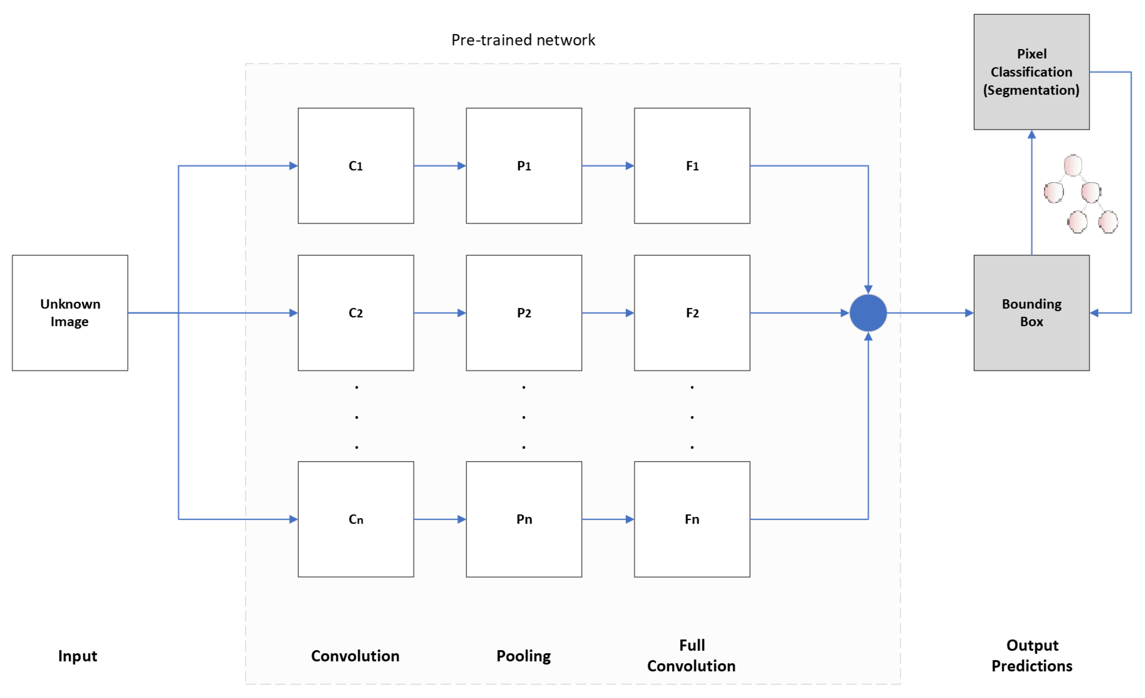
The overall schema of our method is illustrated in
Figure 1. The pre-trained (indicated by the light gray background in
Figure 1) multi-layer neural network is composed of the convolution layer (
), the pooling layer (
, and a full convolution / connection layer (
). The convolution layer contains of
n filters, each of which is weighted matrix. These filters are convolved with the input image, and subsequently transformed with a non-linear activation function. This way a number of feature maps are produced, albeit with redundant information. To reduce redundancy a pooling layer (
) summarizes feature maps into smaller local subsets. The convolution and pooling layer are led to the fully connected layer (
) for categorization; that is the production of the bounding box of a predicted segmentation area. This bounded box area is further refined by means of the Eigen tree decomposition (dark gray boxes in
Figure 1), enriched by decision criteria for segmenting specific areas of interest (pixel segmentation).
We use a dataset devised from dry-dock conditions described in
Section 2.1, both for training and testing input of a convolution neural network, namely YOLOv8, thus produce a new model for corrosion based on our dataset. This produced model is then used for output prediction. The implementation of the YOLOv8 trained model is described in
Section 2.2. The output prediction (bounding boxes) are refined and segmentation of pixels is produced by means of the Eigen decomposition module (
Section 2.3).
2.1. Data
In order to explore performance characteristics of the selected methods, we use the corrosion images dataset for marine vessels in dry-dock conditions[
12,
16]. The dataset incorporates several artifacts due to environmental conditions (e.g. changing lighting conditions, sky, sea) and objects in front of the hull (e.g. maintenance ladders, rudders) not belonging to the marine vessel surface. The data-set contains: (a) high resolution RGB images of 3799 × 2256 pixels (72 dpi, 24bit depth), (b) low resolution RGB images of 1920 × 1080 pixels (96 dpi, 24 bit depth), alongside (c) labelled (ground truth) images that have RGB triplet values for each pixel that corresponds to corrosion and zero valued elsewhere. The labelled areas in the image are manually annotated by human inspectors, denoting regions of interest characterised by rust but may include areas that are suspected to produce surface rust in the near future.
However, for supervised training required by techniques such as neural nets, a larger dataset would be needed. As such, we split all images in the original dataset (either high or low resolution) into four equally sized images maintaining their original form. We then resize the new split images into bounded 512 × 512 pixels. In effect, the two image sets (high and low resolutions) are re-sized to produce a larger dataset of 930 images of pixel analysis 512 × 512 pixels of 72 dpi and bit depth 24 bit.
2.2. YOLO v8 Trained Model
As previously mentioned, we have used the
YOLO v8 architecture, since it has been known to predicting fewer boxes, and has a faster non-maximum suppression process. The architecture offers five different scaled versions, known as : nano (YOLOv8n), small (YOLOv8s), medium YOLOv8m, large (YOLOv8l), and extra-large (YOLOv8x). We have experimented in training all versions with our dataset under a 60:40 split (training to testing) ratio, for 600 epochs of batch size 1, with early stopping set at 10 epochs. Under these conditions, the YOLOv8l variant produced the best trained models and achieved increased corrosion recognition accuracy, under mosaic augmentation (not enabled in the last ten epochs to avoid bias).
A single-stage object detection model was employed, which performs object localization (position of objects in image frame) and classification within the same network (production of bounding boxes). The trained backbone architecture includes the corrosion feature maps, an aggregation operator (merge corrosion maps), and a head to produce the final predictions in the form of bounding boxes, of some confidence assigned to each box. In effect, the trained model divides each image into grids, and for each grid (equal size) predicts a number of bounding boxes alongside the confidence. The confidence reflects the accuracy of the bounding box, which contains an object regardless of class. The classification score for each box and for every class in training can be combined to produce the probability of each class being present in a predicted box.
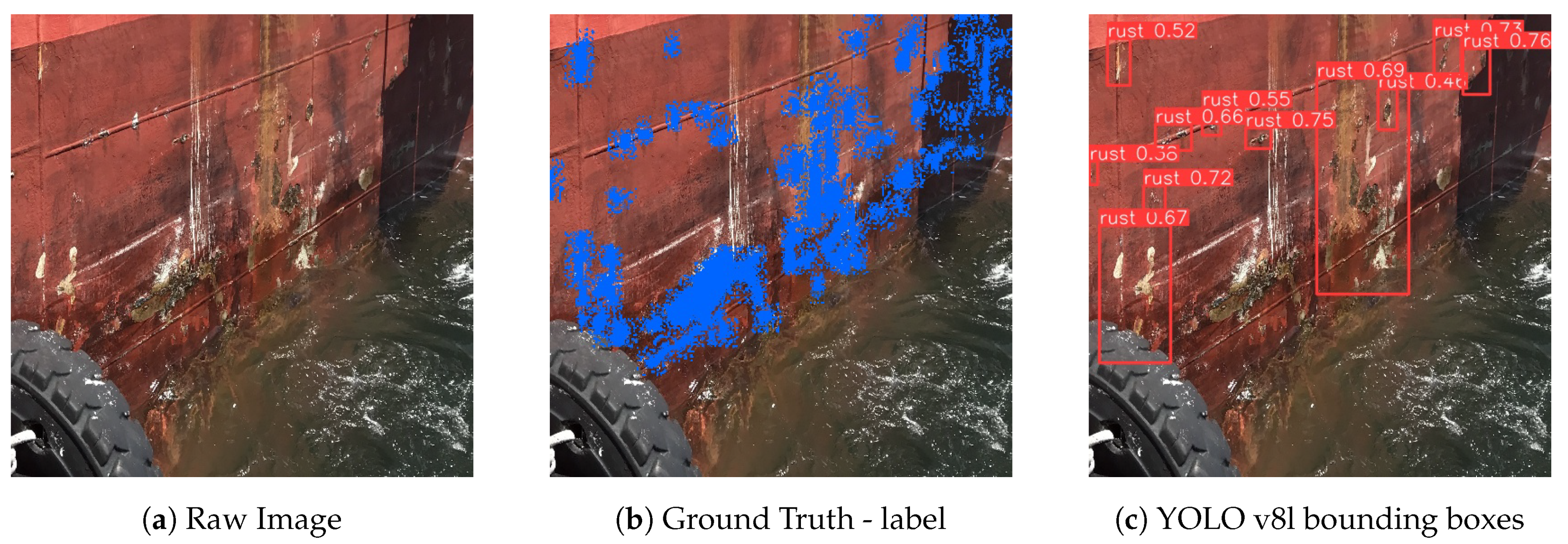
An example output of the trained YOLOv8l model can be observed in
Figure 2(c), alongside the raw image (
Figure 2(a)) and ground truth (
Figure 2(b)). This example visually illustrates the performance of the trained model; that is, the image artefacts (e.g. sea level, block tire) are correctly ignored, alongside the reported confidence for each bounding box. Furthermore, by means of comparison to the ground truth, the produced bounding boxes only include areas of corrosion. Specific performance metrics will be examined in latter sections.
2.3. Proposed Eigen Module (YOLO-Eigen)
Our Eigen module acts upon the YOLO v8l trained model (
Section 2.2) produced bounding boxes (as per example of
Figure 2), in a binary tree structure. The Eigen tree decomposition selects a candidate node and under certain conditions produces a split into leaf nodes. In our case this manifests as a binary slit of two leaf nodes whereas two quantisation levels (
are estimated and each member of a cluster is associated to that of the closest quantisation level [
17]. It is assumed that the mean intensity value of each colour channel is the histogram point with the least variance in the eigen space, leading to a specific quantisation level value
. The quantization level value of each colour channel, and for each node, is defined as
, where
is the number of pixels belonging to some cluster, and
is the number of clusters.
The module is based upon a representation of decision trees which performs binary splits so that an appropriate hyperplane is selected; that is, hierarchically separates data into clusters in a sequence. Inasmuch, current iteration clusters are not re-evaluated in their totality but only in the sequence of a current branch. For a binary split decision tree, this means that the average of square distances of all data points (image pixel quantisation levels ) sequentially generate leaf nodes of new clusters .
In effect, a node split is determined by its eigenvector being that of the largest eigenvalue over all previous nodes, which in turn determines the pixel indices in cluster
that will be assigned into the new clusters
,
. The binary split for node image indices
ℓ association over cluster
is performed using the schema:
In order to identify the leaf node that best captures the corroded regions found within the input frame, the YOLO-Eigen module iterates over the leaf nodes
,
, where
k the pruning invariant depth, identifying the nodes that correspond to the maximum eigenvalue
and maximum entropy
. In the event that
,
point to different leaf nodes, the node of
is eliminated from the candidate pool. Conversely, if both max values refer to the same node, we assume that the selected node converges to the maximum of all entropy values. Since the predicted leaf node contains only pixel indices, the prediction methodology preserves the and reconstructs the predicted frame based on said cluster indices. The handling of eigenvectors
and information entropy
are further described in [
12].
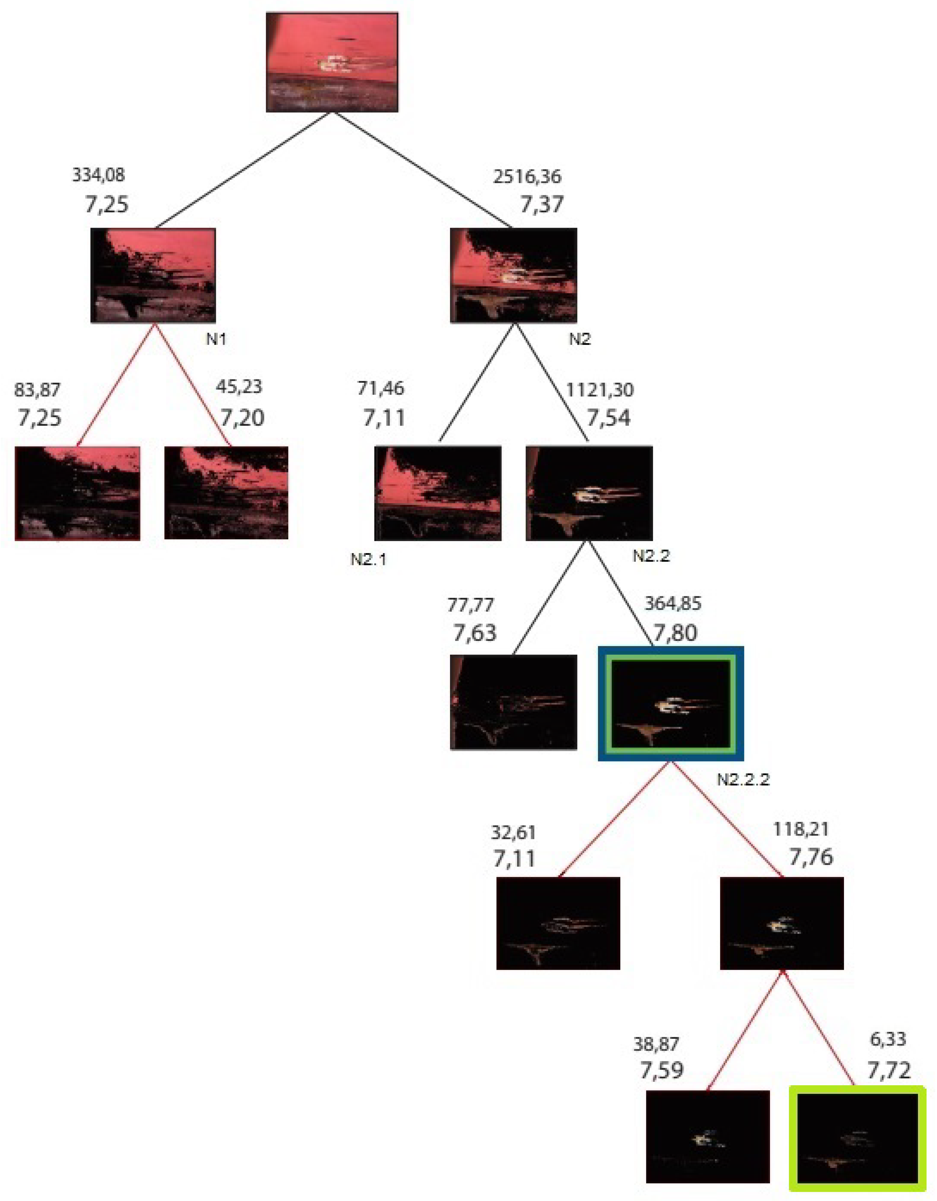
An example of the tree generation can be inspected in
Figure 3. It should be evident that the top image is split into corresponding nodes N1, N2 of eigenvalues (
). Node N2 is of the largest value (i.e. 2516) and thence split into nodes N2.1 and N2.2, producing eigenvalues
. The new node splits will be performed at node N2.2 due to largest eigenvalue (1121). In this example, the tree continues forming in such a way, until tree depth
is reached. Note that for the right hand side direction (RHS) of the tree, the bottom most nodes have an entropy of
and
, with a parent node of
. This means that the leaf nodes do not hold more information than their parent, and are pruned. Similarly, the remainder leaf nodes of entropy
and
do not hold more information than their parent node of entropy
, and are also pruned. In the final step for RHS leafs, the remainder leaf nodes of
and
, hold more information than their parent node of entropy
and are preserved. Since there are no further steps at RHS, the process moves to LHS accordingly. In line with this specific example , the selected `best’ node is framed in green colour, with the ground truth being framed in `blue’ colour. Notice that for the unprunned tree, the selected node is that of light green colouring and has less overall coverage versus that of the ideal annotated ground truth (blue node). However, in the case of the pruned tree the decision criteria identifies a node (green) that coincides to the ground truth (blue). This is a bottom up approach, whereas from all nodes below N2.2 are eliminated, and the selected as dominant (green) node has both the largest information entropy and the largest eigenvalue. Notice that the parent node N2.2 has a higher eigenvalue but lower entropy and thus would not be selected by the decision criteria.
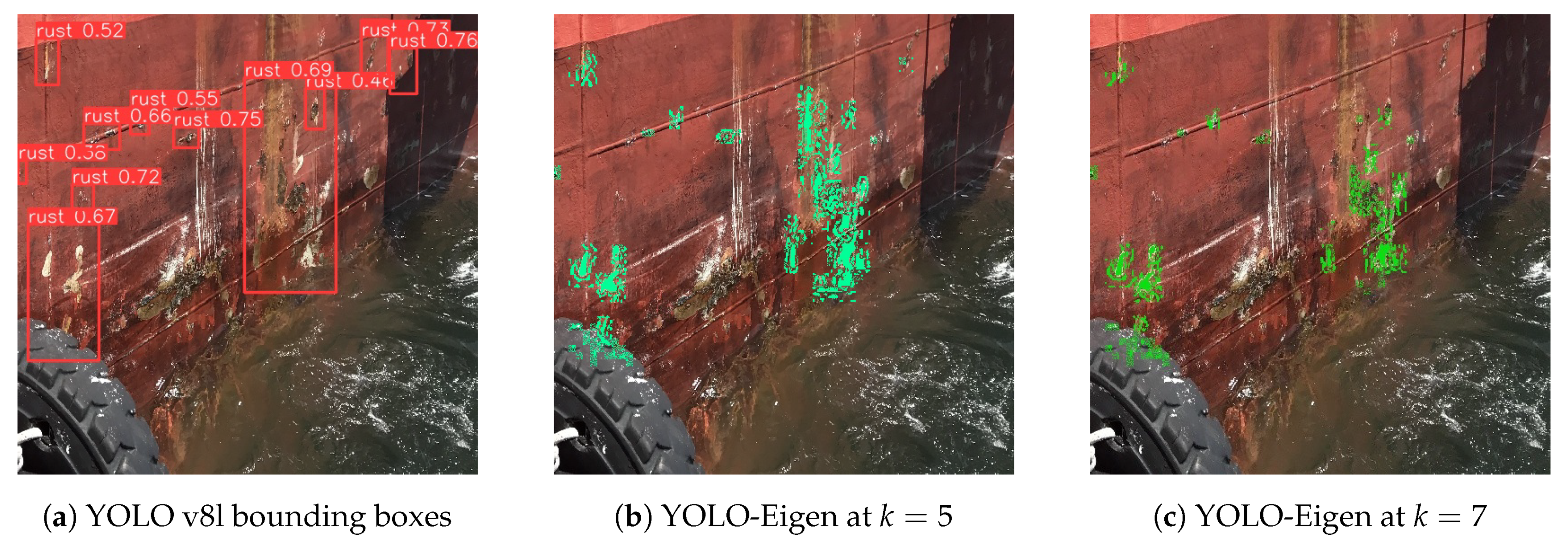
We conclude by expanding upon the example of
Figure 2. The use of our Eigen module refines the trained YOLOv8 produced bounding boxes, and proceeds by means of the decision criteria to the segmentation result is shown in
Figure 4. In this particular example, it should be obvious that refinement of YOLO bounding boxes at Eigen tree
, produces better coverage than for
, at the expense of producing more false negatives (FN). For
there is smaller but more specific segmentation coverage (reduced FN), at the expense of simultaneous reduction in true positives (TP). This example serves as the starting point for our further investigations in
Section 3.
3. Research Findings
We compare our method with standard deep-learning image segmentation methods as provided in freely available implementation, and we train new models from our dataset. All methods used are trained upon the dataset as described in
Section 2.1. In the case of a Bayesian Neural Network (BNN) implementation we use
SpotRust [
3], which relies on a base network derived from
HRNetV2 [
18]. For Convolutional Neural Network (CNN) we use the optimised implementation
U-Net [
19] through the Sensitive Residual Network blocks (SEResNet). As previously mentioned our hybrid method uses a CNN implementation of
YOLO v8 [
20] for bounding the areas of corrosion interest, and subsequently segments these areas using the Eigen decision tree hierarchies.
The U-Net implementation was trained and tested under a split of the dataset using the SEResNet, which incorporates Squeeze-and-Excitation (SE) blocks that enhance the network’s ability to capture and utilize information. n principle, this is expected to lead to improved performance in image segmentation, distinguishing between true positive/negative and false positive/negative pixel areas, depending on the number of SE blocks used. In our case we have reported results from use of 18 and 34 SE blocks. Furthermore, we utilized a sigmoid activation function and the Adam optimizer, with binary cross-entropy loss function enabled for training the model. The learning rate was set at for 50 epochs.
The BNN implementation (SpotRust) was trained and tested under a training to testing split, using the variational inference (VI) as well as Monte-Carlo dropout (DO) methods. The drop out rate was set at , a learning rate at , and max epochs at 550. However, it should be noted that despite model fine-tuning to our dataset, the produced models the dataset Gaussian noise increased the aleatoric uncertainty. Both variational (VO) and Monte Carlo (MC) models produced outputs of reduced performance.
The YOLO-SAM implementation consists of using our trained YOLO v8l backbone (
Section 2.2), and enforce segmentation by means of the Segment Anything (
SAM) methodology [
21]. The SAM model was configured to run inference via CPU utilisation and for each extracted bounding box that the trained YOLO model will produce on a single image. We then prompted the input of the SAM model by identifying the corresponding coordinates of the bounding box within the label image. However, SAM is a computationally expensive model and there were some images where the model was unable to produce predictions due to RAM constraints. Thus, in the event of RAM depletion, predictions of classified images were set as empty images; i.e. no regions of interest (ROI) found. This can most likely be attributed to the complexity of the scenery found within the input ROIs and their corresponding labels. To minimize the number of affected images, morphological closing on the prompt labels has been applied, with various kernel sizes. This operation was performed until either the model produced an output, or the kernel size reached the same size as the ROI in question.
3.1. Performance Metrics
To assess the performance of corrosion detection, the pixel coordinates of corrosion in an image under investigation are found by comparison to the ground truth annotated images. This is performed by applying the labeled image mask on the input raw image thence generating the dominant cluster result. The pixels defined as `True Positive’ pixels (TP) of a cluster are those that match the labeled mask, and `False Positive’ pixels (FP) are those that do not fall within the labeled mask. Inasmuch, TP explores the number of pixels in the image that are correctly identified as being corrosion; TN presents the number of pixels in the image that are correctly identified as not being corrosion; FP indicates the number of pixels in the image that are incorrectly identified as corrosion; and FN indicates the number of pixels in the image that should be identified as corrosion but are not. Under the aforementioned pixels’ definitions, we employ specific metrics that measure: sensitivity, specificity, precision, accuracy, and significance (i.e. the f-score).
Sensitivity is defined as the measure of the number of pixels that were correctly predicted, with respect to the incorrectly predicted as negative pixels. The expression for the described metric is:
Specificity is defined as the measure of the number of pixels that were incorrectly predicted, with respect to the correctly predicted as negative pixels. The expression is:
Precision is defined as the measure of the number of pixels that were predicted correctly, out of total positively predicted pixels. The expression is:
Accuracy is defined as a measure of the number of pixels predicted correctly (either positive, or negative) out of all possible predictions. The expression is:
The
f-score is a metric that relates the calculated sensitivity to precision or accuracy instances. It is a special case of the harmonic mean, of the measures as expressed in Equations
2, by using that of Eq.
4 or
5. It measures the relative significance of the results in terms of a method’s precision or accuracy given its sensitivity. The expression is:
These performance metrics can be though of as constituting a standard (in the machine learning literature) confusion matrix of `observability’ versus `predictability’. T’That is to say, the sensitivity metric relates to how sensitive the predicted pixel segmentation is to false negatives (FN), while the precision metric relates to how precise the segmentation is upon observing false positives (FP). This leads to the corresponding precision based f-score, hence the precision significance of the segmentation result. Similar argumentation applies for the accuracy based significance.
3.2. Segmentation Performance
The segmentation performance of all methods can be investigated by means of the average behaviour of pixels correctly and incorrectly classified as corrosion, with example instances provided in
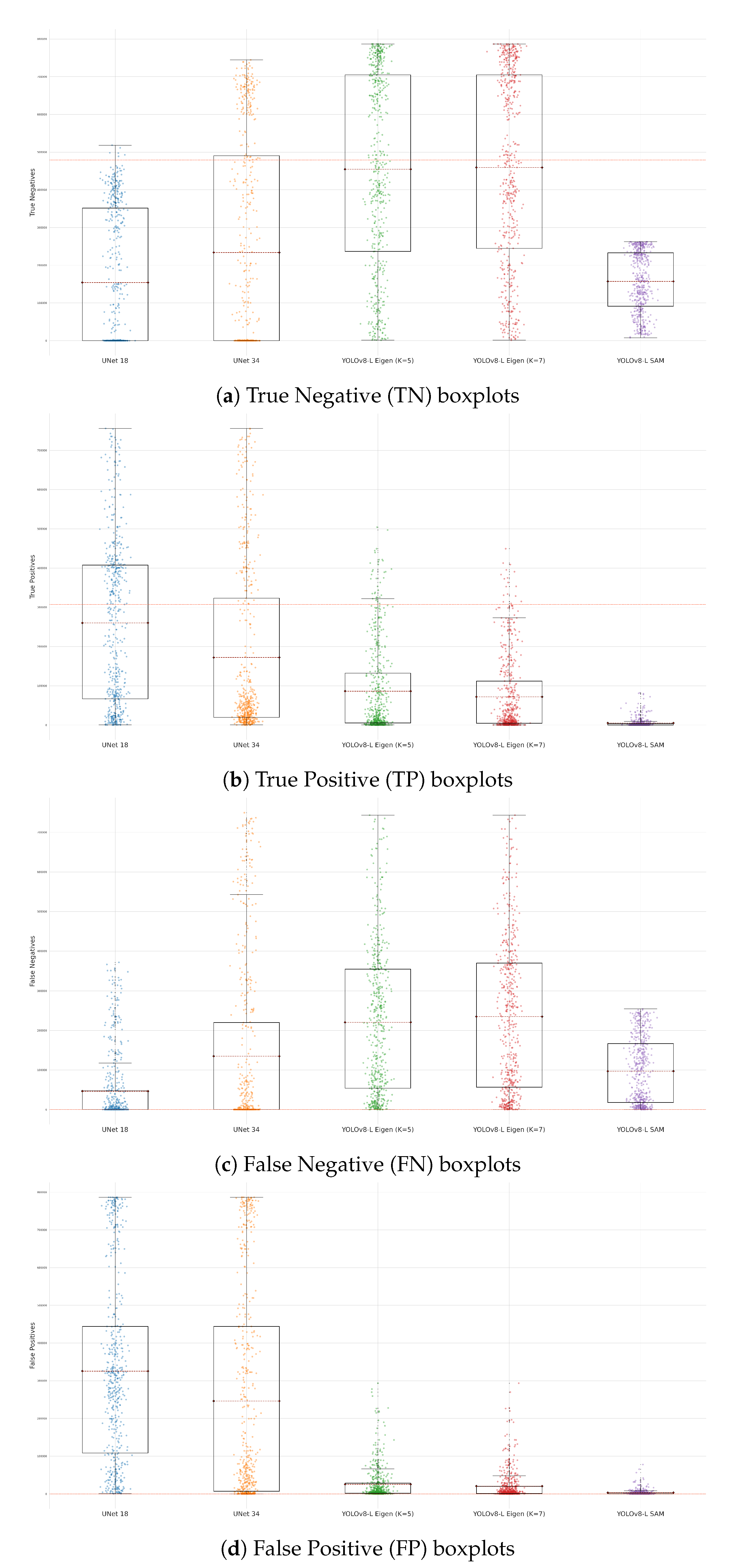
Figure 5. The overall behaviour of correctly classified pixels (TP and TN) and incorrectly classified pixels (FP and FN) is presented in
Figure 6 by means of boxplots. In general, an ideal scenario would be that the output prediction matches the labeled (ground truth) image, as illustrated by example outputs. Consequently, the boxplot presents itself with a spread of one standard deviation length from the average value, and the average value is close to the total average of the entire dataset for True positive or negative predictions, and close to zero for False positive or negative predictions.
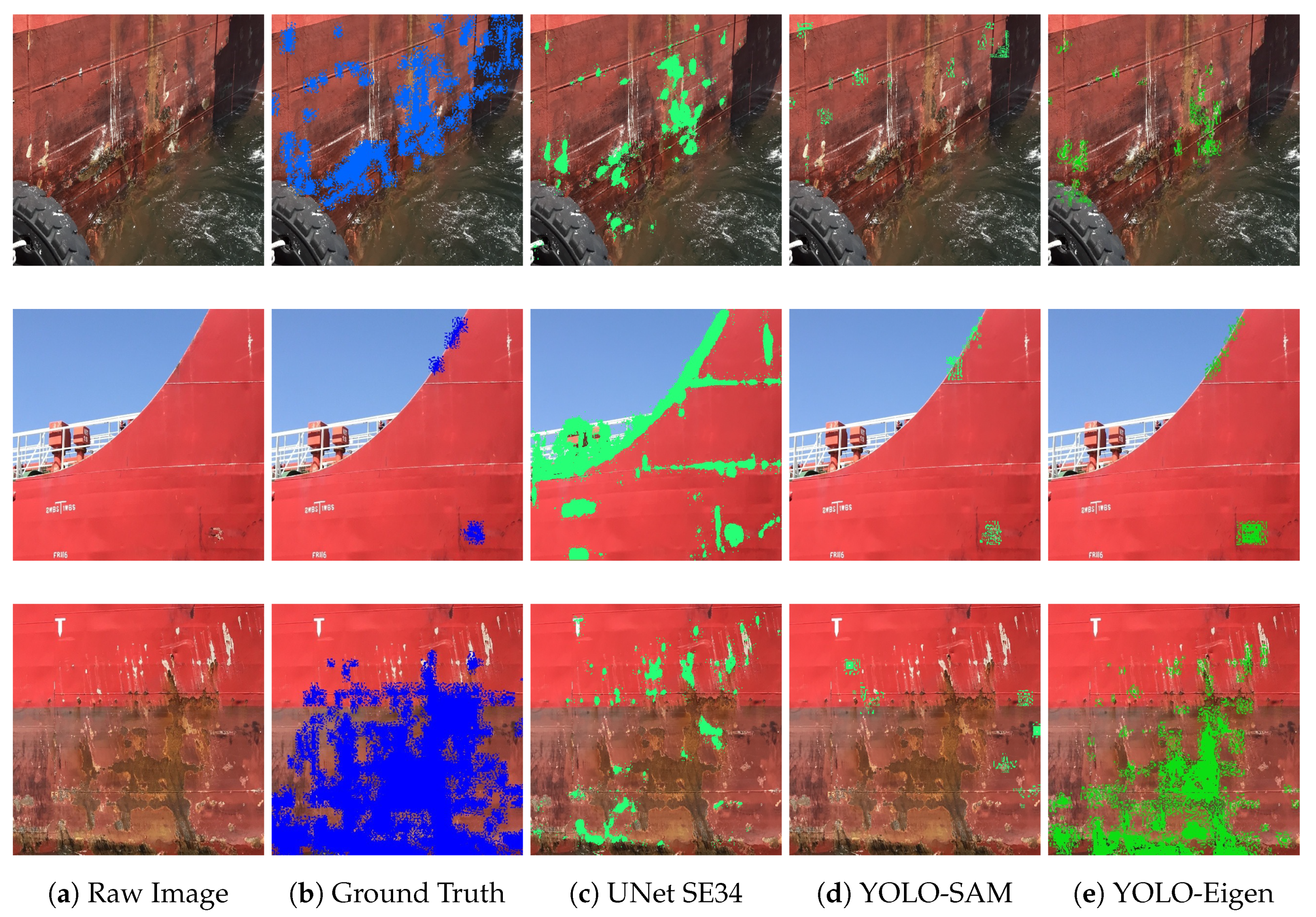
In
Figure 5, three characteristic cases in the dataset are depicted. That is to say, the raw image alongside the ground truth denoted as corrosion (blue pixels), alongside results from different methods. In these specific cases it can be evident in
Figure 5(c) that the UNet model produces an increased number of False Positives (FP), especially in the case of background segments (e.g. sea water, skyline, variable light and shadows). The YOLO-SAM iapproach in
Figure 5(d)appears to lack sufficient coverage of corrosion patterns, thus making it more likely to not produce false positives (FP) or negatives (FN). Conversely, our YOLO-Eigen approach in
Figure 5(e) seems to provide adequate coverage and exhibits high accuracy, particularly when visually compared to the ground truth, even for specific artifacts present in the background.
However, the visual inspection of the examples in
Figure 5, does not provide the full case and the population performance over the whole dataset. As a result we have produced the box plots of
Figure 6. These boxplots and for the defined group of pixels (i.e. FN, TN, FP, TP), illustrate the spread of the detected pixel group (size of box) with respective average value (line inside the box). For True Negative group of pixels of
Figure 6(a), the best performance seems to be that of YOLO-Eigen with the rest of the methods being significantly away from the ground truth TN average. However, the inverse statement is true for the True Positive pixels in
Figure 6(b). This provides us with the indication that the UNet approach is more accurate in its prediction of True Positive, and less accurate in the prediction of True Negative pixels. The YOLO-Eigen approach seems to be more accurate with True Negative as opposed to True Positive pixels. Further to the box plots investigation on the predictive power of the methods with respect to pixel group association, it also be observed in
Figure 6(c) and (d) that the UNet approach produces significant number of erroneously predicted False Positive pixels and significantly less False Negative pixels. The exact opposite is true for our YOLO-Eigen approach, as it produces significantly fewer erroneous predictions of false positives, albeit at the expense of increased false negatives.
It is thus evident in this performance evaluation that in terms of predictive accuracy, and respective significance of predictions, the UNet and our YOLO-Eigen methods produce similar results, as opposed to the BNN and YOLO-SAM approaches. However, an important conclusion is that the UNet approach correctly predicts more positive than negative pixels, albeit at the expense of incorrect predictions of the same type. Therefore, the important conclusion is that the UNet approach correctly predicts more Positive than Negative pixels, at the expense of incorrect predictions of the same type; for our YOLO-Eigen approach the exact opposite seems to be the case.
3.3. Results Analysis
Following our main conclusion from
Section 3.2, it follows that the UNet approach is biased to providing more positive segmentation pixel predictions, as opposed to our YOLO-Eigen approach that generates more negative segmentation pixel predictions. The BNN and YOLO-SAM methods seem to not maintain sufficient coverage of corrosion segmentation when compared to the ground truth. As a consequence we proceed in utilising the metrics of
Section 3.1 to provide specific analysis on the methods’ segmentation results over the entire data-set. These results are reported in
Table 1.
Table 1.
Methods Comparison: all reported values are mean values over the testing dataset portion. Best metric score is reported in Dark Blue colour, with next best score reported in Light Blue
Table 1.
Methods Comparison: all reported values are mean values over the testing dataset portion. Best metric score is reported in Dark Blue colour, with next best score reported in Light Blue
| |
BNN (SpotRust) |
UNet (SEResNet) |
YOLO-Eigen |
YOLO-SAM |
| |
Variational |
Drop Out |
SE-18 |
SE-34 |
|
|
|
| |
|
|
|
|
|
|
|
|
Accuracy (%) |
14.70 |
10.58 |
45.68 |
51.57 |
68.74 |
67.42 |
61.82 |
|
Sensitivity (%) |
83.28 |
86.06 |
50.76 |
56.04 |
28.09 |
25.39 |
16.35 |
|
Specificity (%) |
85.31 |
89.43 |
44.29 |
51.29 |
25.27 |
25.71 |
17.83 |
|
Precision (%) |
11.25 |
11.21 |
34.02 |
41.12 |
77.28 |
73.97 |
64.89 |
| |
|
|
|
|
|
|
|
|
f-score (precision) |
0.19 |
0.19 |
0.41 |
0.47 |
0.41 |
0.39 |
0.25 |
|
f-score (accuracy) |
0.25 |
0.18 |
0.47 |
0.53 |
0.39 |
0.36 |
0.24 |
With reference to
Table 1, it can be deduced that BNN approach is more sensitive and specific in the predictions it produces, but since it does not have sufficient coverage it achieves reduced performance in terms of accuracy and precision. The YOLO-SAM approach seems to over-fit in terms of accuracy and precision, since said predictions seem to be neither specific enough, nor sensitive enough. As a result, the significance score (f-score) is sufficiently smaller than the YOLO-Eigen and UNet methods.
Further to results analysis, it should be evident from
Table 1 that the best results accuracy as well as precision is that of our YOLO-Eigen method, with significance (f-score) comparable to that of the UNet method. One should notice that the UNet method produces comparably good results in all metrics that we have examined. As a result, the UNet method seems to be producing higher significance scores than any other method. This verifies the discussion of
Section 3.2, whereas YOLO-Eigen and UNet were significantly better as opposed to the other methods in terms of true corrosion pixel predictions; albeit, YOLO-Eigen producing more TP versus TN pixel predictions, and vice-versa for UNet.
However, observing
Table 1 and closely compare the significance scores between UNet and YOLO-Eigen, we can conclude that our YOLO-Eigen for
produces the same score as that of UNet SE-18 (both at 0.41), and have a maximum difference of less than 0.09. As a result, and although the UNet approach seems to produce better significance scores upon its accuracy and precision, our YOLO-Eigen approach significantly outperforms all methods in both accuracy and precision. It is thus evident from the results analysis that our YOLO-Eigen approach produces significantly more accurate and precise corrosion segmentation results, with significance score comparable to that the next best method (i.e. UNet).
4. Conclusions
In this paper we have proposed an Eigen tree decomposition module for pre-trained YOLO v8 neural network models, referred to as YOLO-Eigen. The YOLO v8 model was trained via a custom marine corrosion data-set used. We have compared our YOLO-Eigen against other state-of-the-art methods, such as freely available source code for the UNet Convolutional Neural Network, the Bayesian Neural Networks, and SAM as an add-on module to our pre-trained YOLO v8 model. We have hypothesized that due to the multiple pixel quantisation levels of the Eigen Tree decomposition, the YOLO model would produce better segmentation results than other similar in nature techniques for corrosion in marine vessels.
We have verified that for the YOLO v8 pre-trained models our Eigen module segments corrosion on vessel surfaces more accurately and is more precise, with good significance score across the data-set testing inputs. Inasmuch, the next best method (UNet) although it produces higher significance scores it achieves lower accuracy and significantly lower precision performance. However, our YOLO-Eigen method seems to be biased to predictions of higher false positives, as opposed to false negatives that the UNet method produces. It remains a question of risk assessment for the inspection surveyor as to whether having false positive predictions (YOLO-Eigen) is more preferable than having more false negative (UNet) predictions.
As future work we aim to examine further enhancing our technique with three dimensional point-clouds, in the hope that these will correlate to further identifying different types of corrosion. That is, assuming a 3D point-cloud with chroma (RGB) values, it may be possible to identify cracks on the surface, and subsequently correlate to corrosion spread it may also be possible to predict the extent of hull damage and/or predictive maintenance to avoid failure. In addition, we propose future work whereas a full integration of mobile robot arms with computer vision and algorithm described in this paper, to proceed to targeted micro-indentation mapping, and consequently used as a novel procedure to corrosion detection types (e.g. microbial) and predict potential fatigue damage.
Author Contributions
Conceptualization, G.C. and S.V.K.; methodology, G.C.; investigation, G.C. and S.V.K.; data curation, I.T.; validation, I.T. and G.C.; software, I.T. and G.C.; formal analysis, G.C. and I.T.. All authors have read and agreed to the published version of the manuscript.
Funding
This research received no external funding
Data Availability Statement
The raw data used in this study are freely available at [
16].
Conflicts of Interest
The authors declare no conflict of interest.
References
- International Maritime Organization. International Convention for the Safety of Life At Sea. https://www.refworld.org/docid/46920bf32.html. Regulation 3-6: Access to and within spaces in, and forward of, the cargo area of oil tankers and bulk carriers [Last Accessed: May 2023].
- Bonnin-Pascual, F.; Ortiz, A. On the use of robots and vision technologies for the inspection of vessels: A survey on recent advances. Ocean Engineering 2019, 190, 106420. [CrossRef]
- Nash, W.; Zheng, L.; Birbilis, N. Deep learning corrosion detection with confidence. npj Materials Degradation 2022, 6. [CrossRef]
- Ali, A.A.I.M.; Jamaludin, S.; Imran, M.M.H.; Ayob, A.F.M.; Ahmad, S.Z.A.S.; Akhbar, M.F.A.; Suhrab, M.I.R.; Ramli, M.R. Computer Vision and Image Processing Approaches for Corrosion Detection. Journal of Marine Science and Engineering 2023, 11. [CrossRef]
- Coelho, L.B.; Zhang, D.; Van Ingelgem, Y.; Steckelmacher, D.; Nowé, A.; Terryn, H. Reviewing machine learning of corrosion prediction in a data-oriented perspective. npj Materials Degradation 2022, 6. [CrossRef]
- Hussein Khalaf, A.; Xiao, Y.; Xu, N.; Wu, B.; Li, H.; Lin, B.; Nie, Z.; Tang, J. Emerging AI technologies for corrosion monitoring in oil and gas industry: A comprehensive review. Engineering Failure Analysis 2024, 155, 107735. [CrossRef]
- Atha, D.J.; Jahanshahi, M.R. Evaluation of deep learning approaches based on convolutional neural networks for corrosion detection. Structural Health Monitoring 2018, 17, 1110–1128. [CrossRef]
- Forkan, A.R.M.; Kang, Y.B.; Jayaraman, P.P.; Liao, K.; Kaul, R.; Morgan, G.; Ranjan, R.; Sinha, S. CorrDetector: A framework for structural corrosion detection from drone images using ensemble deep learning. Expert Systems with Applications 2022, 193, 116461. [CrossRef]
- Guzmán-Torres, J.A.; Domínguez-Mota, F.J.; Martínez-Molina, W.; Naser, M.; Tinoco-Guerrero, G.; Tinoco-Ruíz, J.G. Damage Detection on Steel-Reinforced Concrete Produced by Corrosion via YOLOv3; A detailed guide. Frontiers in Built Environment 2023, 9, 41. [CrossRef]
- Brandoli, B.; de Geus, A.R.; Souza, J.R.; Spadon, G.; Soares, A.; Rodrigues, J.F.; Komorowski, J.; Matwin, S. Aircraft Fuselage Corrosion Detection Using Artificial Intelligence. Sensors 2021, 21. [CrossRef]
- Das, A.; Ichi, E.; Dorafshan, S. Image-Based Corrosion Detection in Ancillary Structures. Infrastructures 2023, 8, 2412–3811. [CrossRef]
- Chliveros, G.; Kontomaris, S.V.; Letsios, A. Automatic Identification of Corrosion in Marine Vessels Using Decision-Tree Imaging Hierarchies. Eng 2023, 4, 2090–2099. [CrossRef]
- Pimentel de Figueiredo, R.; Nordborg, S.; Bøgh, S.; Rodriguez, I. A Complete System for Automated 3d Semantic-Geometric Mapping of Corrosion in Industrial Environments 2024. [CrossRef]
- Ortiz, A.; Bonnin-Pascual, F.; Garcia-Fidalgo, E.; Company-Corcoles, J. Vision-Based Corrosion Detection Assisted by a Micro-Aerial Vehicle in a Vessel Inspection Application. Sensors 2016, 16, 2118. [CrossRef]
- Nash, W.; Drummond, T.; Birbilis, N. Deep Learning AI for corrosion detection. NACE International CORROSION Conference Proceedings. NACE-2019-13267, 2019.
- Chliveros, G.; Tzanetatos, I.; Kamzelis, K. MaVeCoDD Dataset: Marine Vessel Hull Corrosion in Dry-Dock Images. Mendeley Data, v1 2021. [CrossRef]
- Orchard, M.T.; Bouman, C.A. Color Quantization of Images. IEEE Transactions on Signal Processing 1991, 39, 2677–2690. [CrossRef]
- Wang, J.; Sun, K.; Cheng, T.; Jiang, B.; Deng, C.; Zhao, Y.; Liu, D.; Mu, Y.; Tan, M.; Wang, X.; Liu, W.; Xiao, B. Deep High-Resolution Representation Learning for Visual Recognition. IEEE Transactions on Pattern Analysis and Machine Intelligence 2021, 43, 3349–3364. [CrossRef]
- Ronneberger, O.; Fischer, P.; Brox, T. U-Net: Convolutional Networks for Biomedical Image Segmentation. Medical Image Computing and Computer-Assisted Intervention; Navab, N.; Hornegger, J.; Wells, W.M.; Frangi, A.F., Eds. Springer International Publishing, 2015, pp. 234–241.
- Redmon, J.; Divvala, S.; Girshick, R.; Farhadi, A. You Only Look Once: Unified, Real-Time Object Detection. IEEE Conference on Computer Vision and Pattern Recognition (CVPR); IEEE Computer Society: Los Alamitos, CA, USA, 2016; pp. 779–788. [CrossRef]
- Kirillov, A.; Mintun, E.; Ravi, N.; Mao, H.; Rolland, C.; Gustafson, L.; Xiao, T.; Whitehead, S.; Berg, A.C.; Lo, W.Y.; Dollar, P.; Girshick, R. Segment Anything. Proceedings of the IEEE/CVF International Conference on Computer Vision (ICCV), 2023, pp. 4015–4026. [CrossRef]
|
Disclaimer/Publisher’s Note: The statements, opinions and data contained in all publications are solely those of the individual author(s) and contributor(s) and not of MDPI and/or the editor(s). MDPI and/or the editor(s) disclaim responsibility for any injury to people or property resulting from any ideas, methods, instructions or products referred to in the content. |
© 2024 by the authors. Licensee MDPI, Basel, Switzerland. This article is an open access article distributed under the terms and conditions of the Creative Commons Attribution (CC BY) license (http://creativecommons.org/licenses/by/4.0/).
