3.1. Datasets
To ensure an exhaustive appraisal of the proposed model, it is tested on five datasets spanning three languages: English, Arabic, and German. To comprehensively train models using DL, a certain sample size is needed, which this study does not meet. Therefore, DA is applied to all the datasets. The following paragraphs summarize each of the datasets employed here.
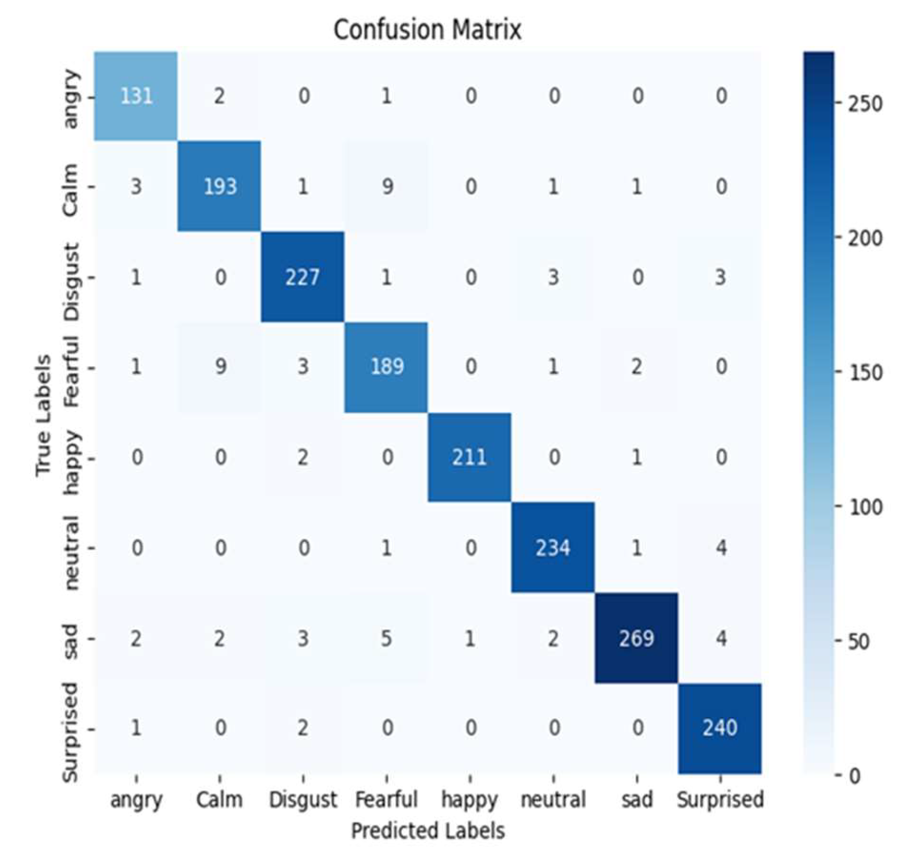
The RAVDESS is a validated multimodal database containing emotional speech and song recordings. The database comprises 7,356 audio files recorded by 24 professional actors, divided equally between men and women. The actors were recorded speaking two linguistically neutral statements while adopting a neutral or standardized accent to minimize the influence of regional variations on the emotional content of the speech. By having professional actors record these controlled statements, high-quality emotional portrayals devoid of confounding regional accents were obtained. RAVDESS provides a substantial corpus of emotional speech and song for research and development in fields such as affective computing. The standardized validation protocols embedded in the dataset aid in comparative benchmarking and reproducibility across studies. Additionally, the spectrum of emotions conveyed by the speech in this dataset encompasses an array of affective states, including but not limited to tranquility, satisfaction, elation, melancholy, indignation, trepidation, astonishment, and revulsion [
25]. Each expression is associated with a distinct level of emotional intensity, ranging from neutral to normal to strong.
The EMO-DB was created by the Technical University of Berlin Institute of Communication Science [
26]. It is a free German emotional speech database [
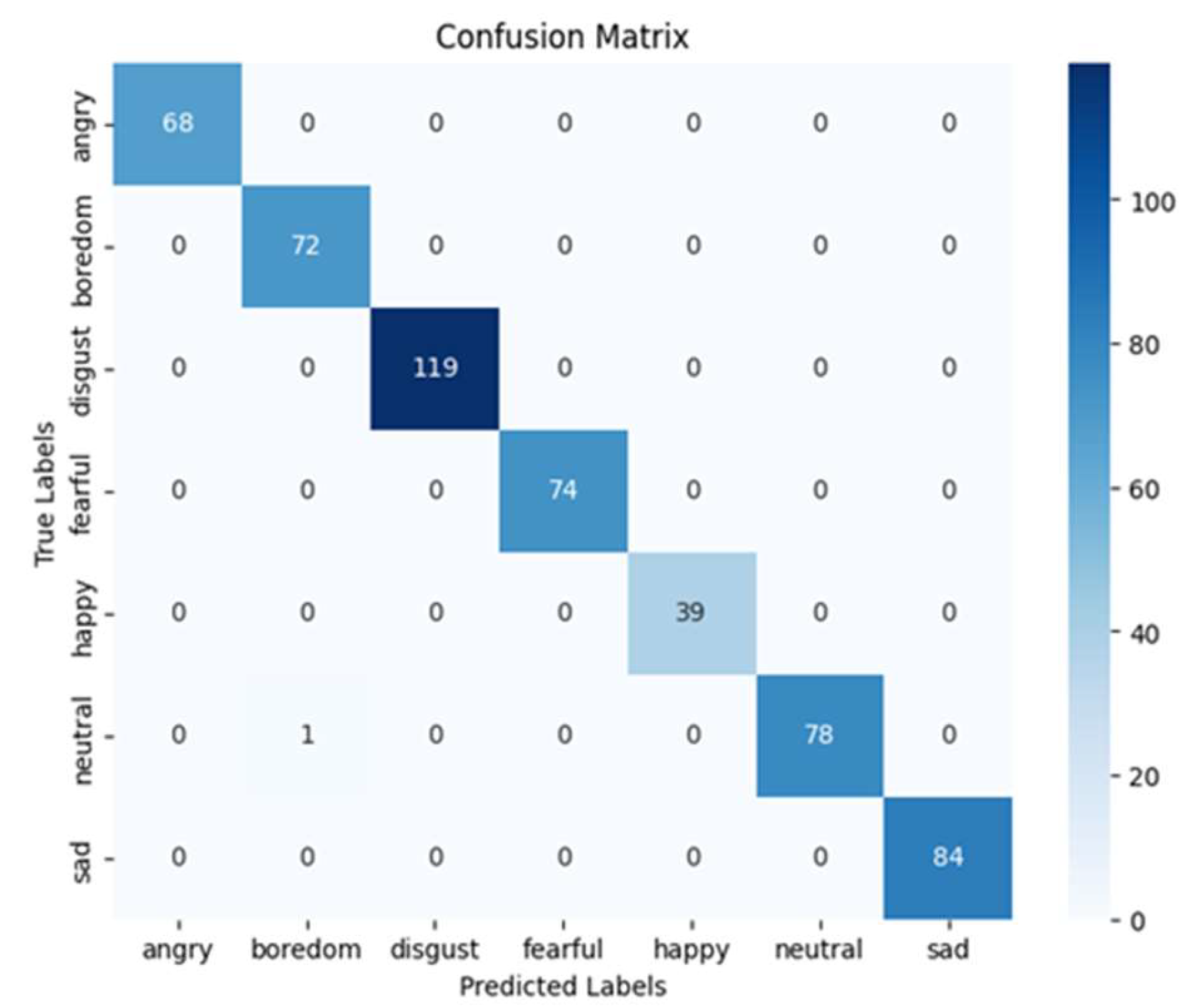
26] that includes 535 context-variable sentences used in everyday communication delivered by 10 expert actors (five men and five women) who, while speaking, simulated either happiness, anger, anxiety, fear, boredom, disgust, or neutrality. The 48-kHz data were down-sampled to 16-kHz.
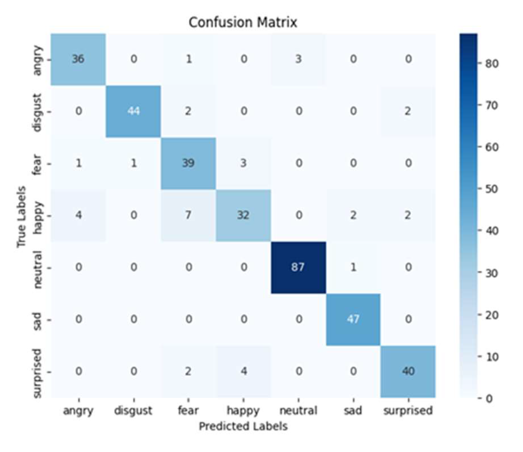
The SAVEE dataset comprises 480 utterances in British English recorded by four male postgraduate students and researchers at the University of Surrey, all of whom were native English speakers aged between 27 and 31 [
27]. Seven different emotions were expressed through these utterances (happiness, sadness, surprise, fear, disgust, neutral, and anger), with sentences from the phonetically balanced Texas Instruments/Massachusetts Institute of Technology corpus chosen for each emotion (See
Table 1).
The
IEMOCAP was developed by the Signal Analysis and Interpretation Laboratory (SAIL) at the University of Southern California. This database represents an acted multimodal, multi-speaker collection of data. The dataset spans 12 hours and includes videos, audio, face tracking, and text transcriptions of paired performances in which actors try to elicit a particular feeling from the viewer using a combination of improvisation and prepared scenes. Multiple annotators contributed labels to the IEMOCAP database, classifying the data according to dimensional labels, including valence, activation, and dominance, as well as category labels, such as anger, happiness, sadness, and neutrality [
28].
The SHEIE dataset is a unique emotional speech dataset developed to test the model proposed herein. It features real interactions from the realm of higher education and focuses on instructors. Recognizing the scarcity of datasets comprising genuine interactions, this dataset was designed to address the gap in existing speech emotion studies. It includes six universal emotions: anger, happiness, sadness, excitement, boredom, and neutrality. The data were collected from the various synchronous online lectures held for the Computer Science Department at King AbdulAziz University and the Islamic Studies Department at Al Jouf University, which were delivered in both Arabic and English. The dataset contains a total of 20 hours and 50 minutes of speech data from 19 lecture sessions. The audio data were collected by two instructors (one male, one female) and were carefully segmented and labeled. Developing the SHEIE dataset involved a four-step process. First, it was determined that real interactions rather than acted emotions would be recorded during live lectures via the Blackboard e-learning system. Second, the emotions represented in the dataset were selected based on their relevance to an instructor’s experience during a lecture. Third, volunteer instructors from the two universities were selected to participate in the study, and they provided the speech data via their lecture recordings. Finally, the emotions in the dataset were labeled based on self-reporting by instructors, which meant selecting an emotion from a prompt every ten minutes during their lectures. The time interval was chosen in response to research indicating that student attention begins to wane around the ten-minute mark. The SHEIE dataset underwent extensive pre-processing, which included splitting the data into ten-minute segments, manually labeling the emotions, cleaning the data to exclude noise and unwanted sounds, and normalizing the data into equal three-second intervals. This produced a total of 7,515 audio files, each labeled with a specific emotion and formatted for use in SER research: 490 files for anger, 1,888 files for happiness, 1,439 files for sadness, 516 files for boredom, 1,654 files for excitement, and 1,528 files for neutrality.
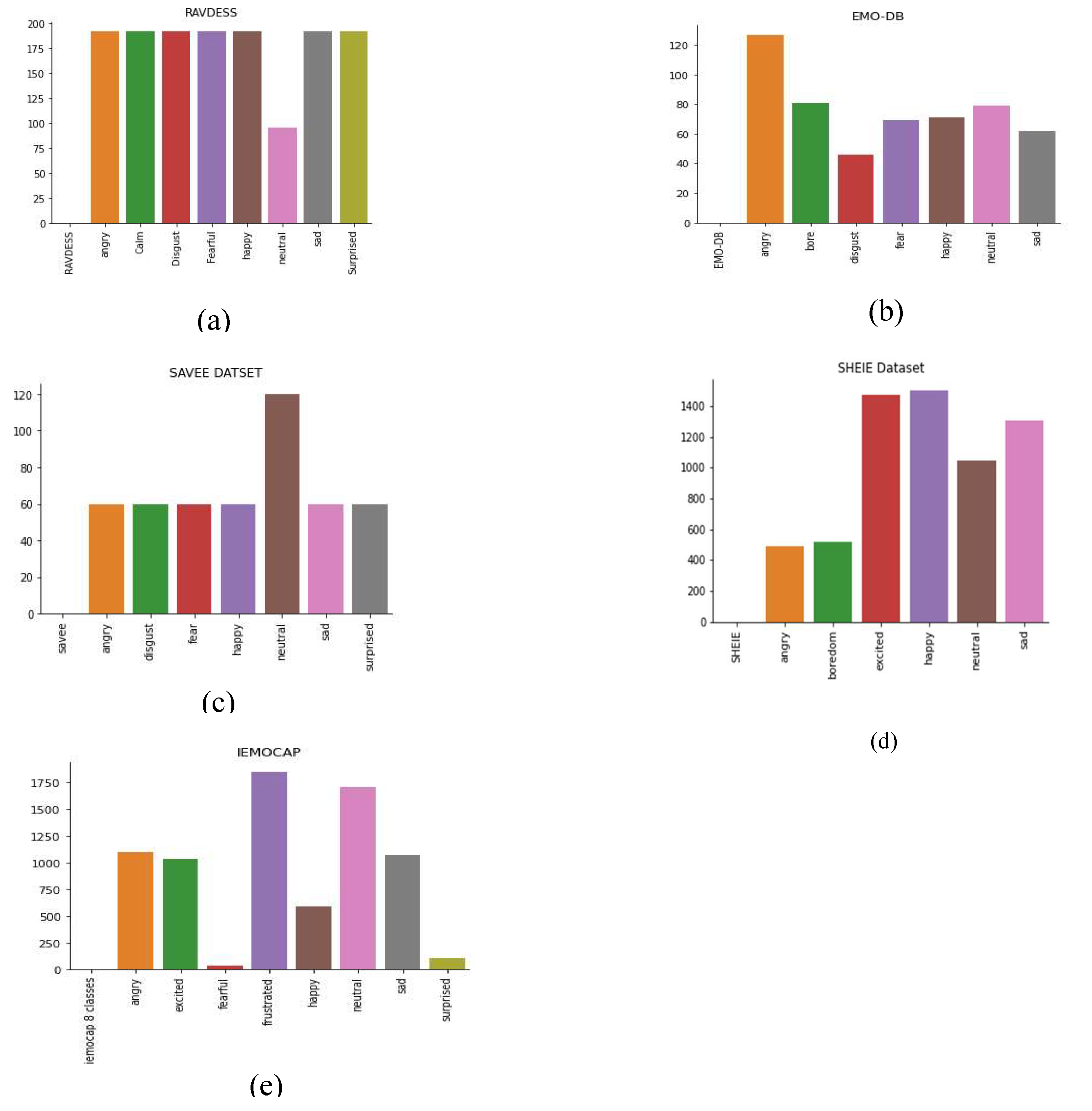
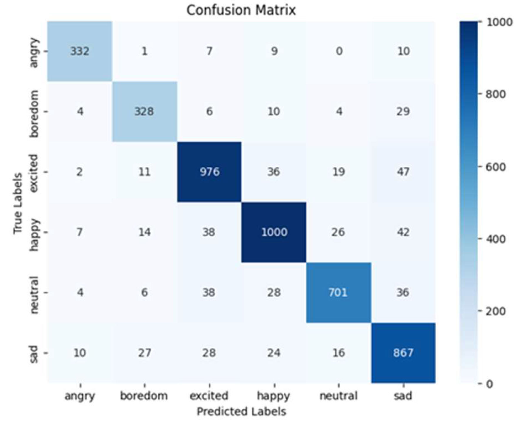
Figure 2 details the distribution of the different emotional classes in these five datasets. Some emotional classes occur more often in most datasets, while others demonstrate the inverse. Thus, there are imbalances in the emotional class distributions across the datasets, indicating the need for DA before model training.
Table 1 presents a description of all five datasets as well as the distribution of the classes in these datasets.
3.2. Data Augmentation
DA is essential for assessing SER model performance because SER systems often lack sufficient and diverse training data. This is observed in the imbalance between emotional classes in this study’s datasets as shown in
Figure 2. Therefore, speed, pitch, noise, and time stretching are used to generate variant data to give the model more context. This DA greatly improves the ability of SER systems to generalize and recognize emotions from speech under uncontrolled and varied conditions [
29]. DA reduces overfitting, making the SER model more stable during the training process.
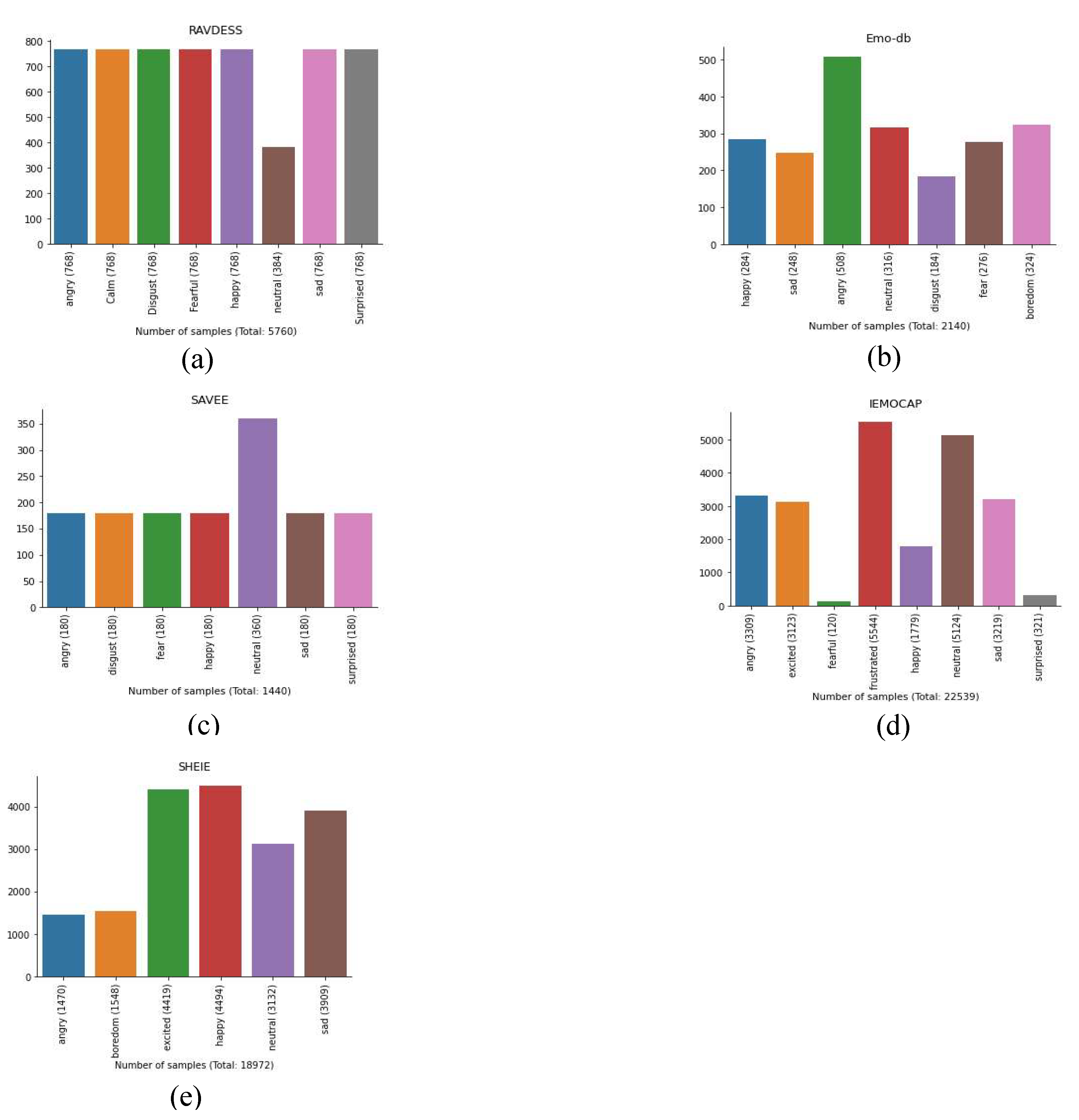
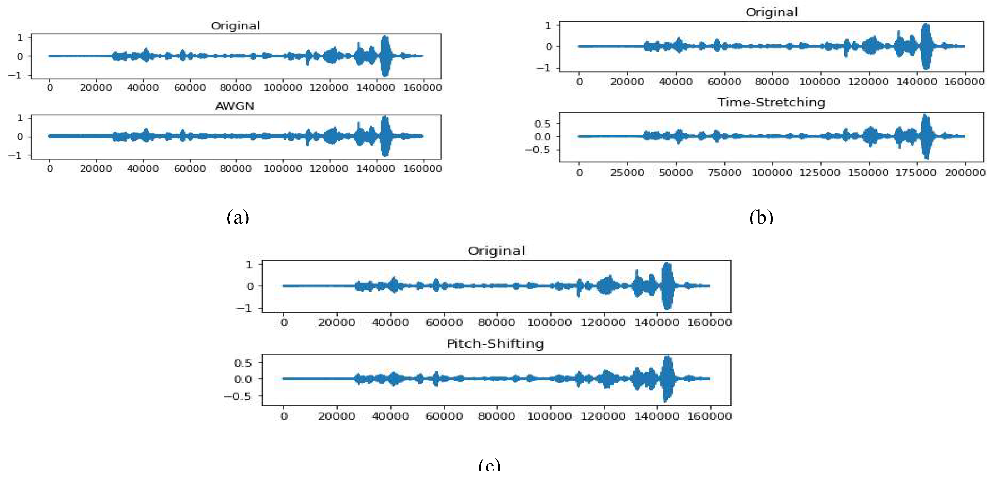
Figure 3 illustrates the influence of DA on SER tasks for this study’s five different datasets. DA techniques, such as adding additive white Gaussian noise (AWGN) to the samples, are employed to balance class distributions across these datasets, effectively addressing the imbalances in the class distributions. Furthermore, a custom noise function is used to add AWGN to the samples, as shown in
Figure 4. This results in DA by adding random noise that is multiplied by 0.01 to the data. In addition, time stretching is used to stretch the data by the given rate, and the pitch shift function is applied with factors of 0.5 and 0.6. Time shifting is also employed using a custom shift function that incorporates the data, sampling rate, maximum shift value, and shift direction. A random shift value within the maximum shift value that is multiplied by the sampling rate is also generated. The shift value is negated for the right shift direction, and if the direction is labeled as “both,” the direction is deemed to be random. The positive shift values set the first shift values of the DA to 0, and the last shift values are 0 if the shift values are negative, resulting in DA.
Figure 4 indicates the changes in the waveforms after applying these DA techniques.
3.3. Feature Extraction
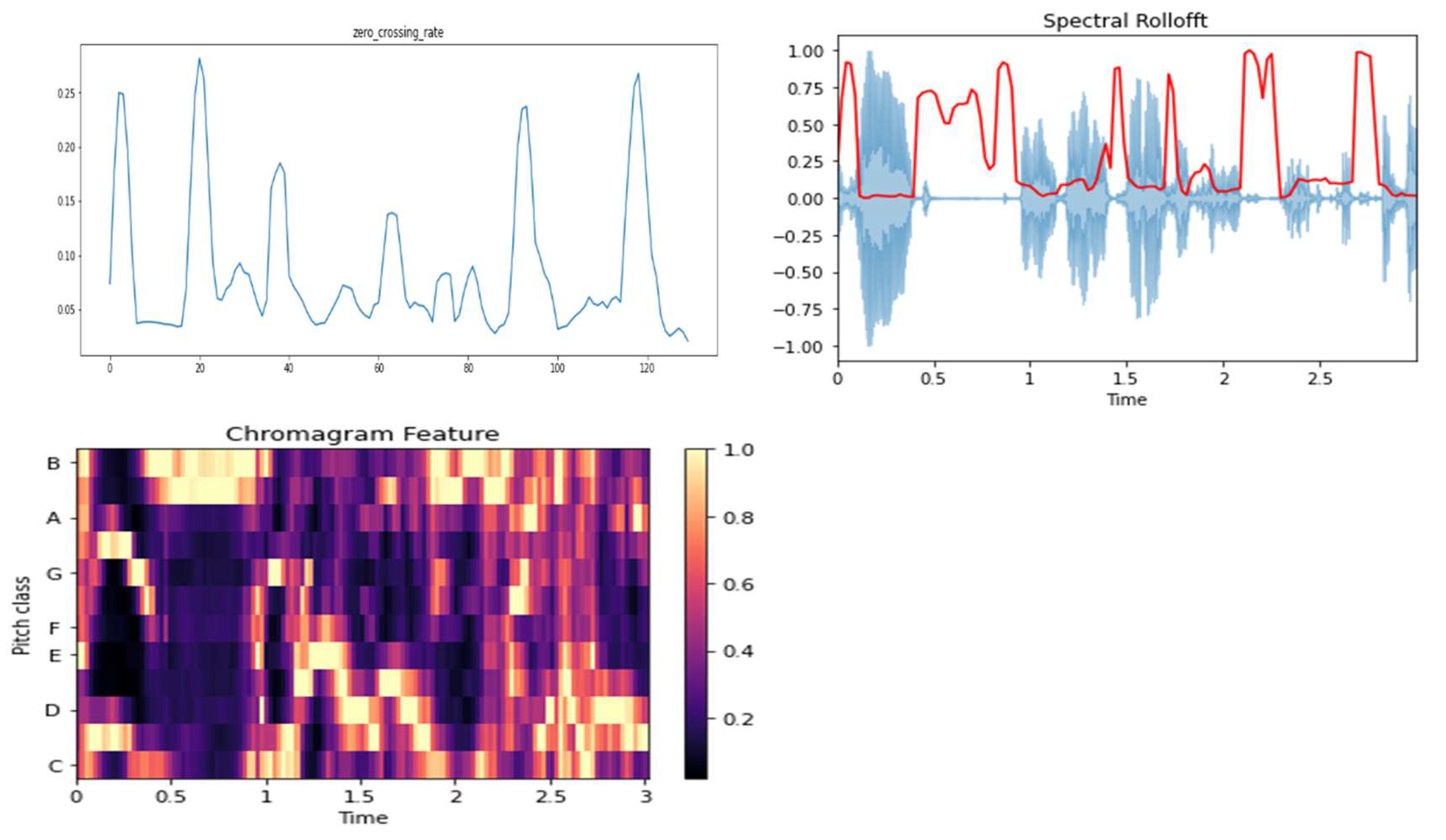
SER extracts features from speech waves to determine a person’s emotional state because transforming speech into features or parameters allows for the determination of emotional characteristics. Features that can be extracted from the time domain include ZCR, energy, and amplitude, which can be used to identify anger and excitement by revealing speech rate and volume. Pitch, formant, and other features can be extracted from the frequency domain, with ZCR, chroma, and roll-off representing some of these features, as
Figure 5 shown. Formants (the vocal tract's resonant frequencies) reveal the shape of the vocal tract, which determines the characteristics of articulated speech sounds. Pitch (the perceived fundamental frequency of a sound) can indicate emotions such as fear and surprise. MFCC, spectral contrast, and chroma also affect the spectral domain [
30]. MFCC offer the best approximations of the human ear’s nonlinear frequency perception and represent a sound’s short-term power spectrum. Thus, they allow systems to more effectively understand emotions due to the systems acting like a human. This means that combining features from different domains guarantees a complete speech signal representation, allowing SER systems to identify emotions accurately and precisely.
ZCR measures how often a signal crosses the zero axis by determining signal sign changes per frame [
31]. As such, it denotes the total number of times the wave flips from positive to negative, and it is contrariwise distributed by frame. Mathematically, ZCR can be determined using the following equation:
where s is a signal of length (T) and 1R<0 is a sign function.
A
chromatogram visualizes audio by mapping frequencies onto 12 bins that match the 12 semitones of an octave using Chroma features [
32]. This compresses pitch content into time windows, enabling music analysis applications to recognize chords and harmonic similarity despite timbre and instrumentation changes.
The Mel spectrogram visualizes audio signals by mapping frequencies onto the Mel scale, which aligns with human hearing. This technique captures important sound characteristics, facilitating its widespread use in speech and audio processing.
Spectral contrast, centroid, bandwidth, and roll-off are features extracted from sound signals. The differences in the levels between spectrum peaks and valleys can reveal a sound’s timbre, while the spectrum’s “center of mass” (also called the spectral centroid) can indicate sound brightness. Additionally, spectral bandwidth indicates a sound’s spectral shape by measuring the spectrum’s spread around its centroid, with spectral roll-off used to determine a sound’s high-frequency content.
RMS is a feature that can be extracted from a speech wave and used in SER tasks [
33]. It is used to measure the energy of a signal and provides information about the overall loudness of the signal.
MFCC is used in SER applications to parametrize speech signals generated by the Mel spectrogram. This scale matches the human auditory system more closely than linear frequency bands. To obtain the MFCC, the Mel spectrogram is transformed using discrete cosine transform (DCT) [
26,
27] These coefficients capture speech signal characteristics and are resistant to timbre and instrumentation changes. This process entails determining the energy band of the speech wave, mapping the power spectrum onto the Mel scale using corresponding deltoid windows to obtain the Mel spectrogram logarithm, and applying the DCT to this logarithm to obtain the MFCC. The formula for mapping a frequency (f) in Hertz to a Mel frequency (m) is as follows:
The inverse formula for mapping a Mel frequency (m) to a frequency (f) in Hertz is:
Emotion classification studies typically use 40 MFCC coefficients for feature extraction, but a more nuanced representation of speech data using more coefficients can improve the detection of emotional states. MFCC, especially when combined with RMS and ZCR, has performed well in the complex task of SER [
28,
29].
3.4. Proposed Model
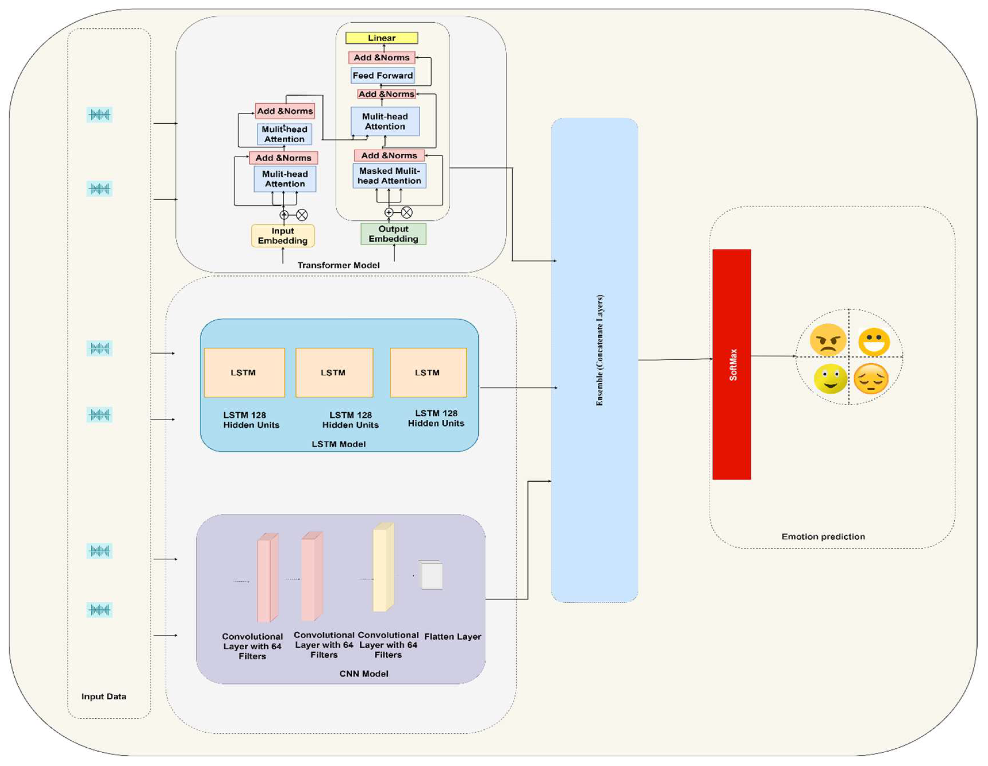
This study’s methodology centers around the construction of an ensemble model that combines Transformer, CNN, and LSTM architectures. Transformer models use self-attention mechanisms to extract contextual features from input sequences, CNN filters extract local temporal features from input sequences, and LSTM models infer long-term dependencies from input sequences using recurrent connections. Therefore, in the study context, the Transformer self-focuses on the interconnectedness of the input elements regardless of sequence, the CNN layers identify the local audio feature patterns, and the LSTM layers capture and learn the long-term dependencies and temporal relationships within the audio sequences. LSTM layers use a series of gates (input gate, forget gate, and output gate) and a memory cell to selectively retain, update, or forget information from previous time steps, enabling them to effectively model and learn from long-term dependencies in the input sequences. The outputs of these three models are then merged and input into a dense final layer for classification, as
Figure 6 shows. Thus, these architectures are combined to determine a feature of the input sequence that accounts for contextual, local temporal, and long-term dependencies. The SoftMax activation function in the dense layer classifies the combined feature representation to produce the final output. The transformer model features three Transformer block layers that contain multi-head self-attention layers and feedforward neural networks (FFNNs). The multi-head self-attention layer embeds 64 units and eight heads, and the FFNNs have 64-unit hidden layers with rectified linear unit (ReLU) activation functions. The CNN model comprises four Conv1D layers with 64 filters and three kernel sizes, with the ReLU activating each Conv1D layer. The flatten layer then flattens the last Conv1D layer outputs, which comprise three 64-unit layers. The first two LSTM layers then return the sequences, with the last layer returning the final hidden state. Then, the final output for emotion classification is generated by concatenating the outputs of the Transformer, CNN, and LSTM architectures and running them through a dense final layer comprising six to eight units and a SoftMax activation function.
- 1)
Transformer Block: Transformer DL models use self-attention mechanisms to focus on different words in the input sequence when producing an output, with the Transformer block using multi-head self-attention to focus on different positions and understand data. FFNNs and dropout layers reduce overfitting, with layer normalization stabilizing learning [36].
The matrices W_Q, W_K, and W_V are subject to training and are capable of being modified by the learning process. Furthermore, attention scores (S) are calculated by multiplying the query and key matrices by the square root of their dimension using the following equation:
W denotes the SoftMax (S), which yields the attention weights, and the attention layer output is a weighted sum of the value matrices: Z = WV.
The FFNN comprises a nonlinear activation function and two linear transformations: W_1, b_1, W_2, and b_2. These denote the adjustable weights and biases for the attention layer. The FFNN outputs are residually connected by adding the input to the output using the following equation:
Layer normalization is the process by which the feature dimension input is normalized according to the attention layer and FFNN output using the following equation:
Y = (X – mean(X))/std(X). * gamma + beta (trainable scale and shift parameters).
The Transformer block in this model comprises an architectural component that accepts a feature vector of size (192, 1) as input (see
Table 2). It consists of a multi-head self-attention mechanism and an FFNN, each of which employs residual connections and layer normalization. In addition, the multi-head self-attention’s embed_dim and num_heads parameters represent the size of the input embeddings and the number of attention heads. Each attention head individually processes the input, allowing the model to concurrently learn different types of information from a singular input sequence. In this mechanism, the query_dense, key_dense, and value_dense are the dense layers that transform the inputs into their corresponding query, key, and value vectors. These vectors are further separated into different heads in the separate_heads method, ensuring parallel and independent computations for each head. The call method subsequently orchestrates the self-attention mechanism’s computation flow by calling the previous components in order. After these computations, the combine heads dense layer merges the outputs from all the attention heads back into the original embedding dimension. The Transformer block also features an FFNN characterized by ffdim, which denotes the size of its hidden layer. To prevent overfitting, two dropout layers that are defined by rate are employed. The FFNN, denoted as ffn, essentially comprises two dense layers: The first applies a ReLU activation function; the second, which is the same size as the embed_dim, applies none. Post ffn, the output enters another dropout layer and residual connection before undergoing normalization using a second layer normalization layer. In summary, the Transformer block transforms the input embedding and outputs a transformed embedding of the same size that has tunable hyperparameters, such as the number of attention heads and the size of the hidden layer in the FFNN. To prevent overfitting, two dropout layers with a rate defined by the hyperparameter 'rate' are employed. The feed-forward network (FFN) in the Transformer block consists of two dense layers: the first one applies a "relu" activation function, and the second one, which has the same size as 'embed_dim', applies no activation function. The FFN is applied to the output of the multi-head attention mechanism, which computes the attention weights between all pairs of positions in the input sequence using multiple attention heads. The purpose of the FFN is to process the concatenated output from the different attention heads, allowing the model to capture more complex dependencies and transformations. After the FFN, the output traverses another dropout layer and undergoes a residual connection, followed by normalization using a second LayerNormalization layer. The Transformer block transforms the input embedding, outputting a transformed embedding of the same size, with tunable hyperparameters like the number of attention heads and the size of the hidden layer in the FFN.
- 2)
CNN: After the Transformer block, the CNN is used, which comprises two Conv1D layers. The (192, 1) feature vector feeds these layers. Each filter (f) is a vector of the weights of size (k), which denotes the kernel size. The output of the convolutional layer at position I is determined using the following equation:
If padding is utilized, the input sequence is expanded with zeroes before the filters are applied. Additionally, when a nonlinear activation function, such as ReLU, is employed, it is implemented on every individual element of the convolutional layer’s output.
The Conv1D layers comprise 64 filters and three kernel sizes. The padding technique known as “same” is utilized to pad the sides of the input to achieve a width that matches that of the output. The ReLU activation function then introduces non-linearity to the model by producing the input value as an output if it is positive and zero if it is negative. The CNN layers then use filters to obtain the local features from the input vectors through convolution.
- 3)
LSTM: The model’s long-term LSTM layers process the sequence data, with the LSTM accepting the original (192, 1) input feature vector. The LSTM comprises two 64-unit layers. The first outputs its hidden state at every time step because the return sequences are labeled “True,” and the text LSTM layer receives each output. This means that this setting is required when stacking LSTM layers. The second LSTM layer does not include this parameter, so it only returns the last output, which is then fed into dense layers to obtain the final predictions. Notably, LSTM networks can predict sequence data, remember information, and avoid the vanishing gradient problem of traditional recurrent neural networks.
For each time step (t), the LSTM simultaneously receives x_t from the input sequence as well as c_t-1 and h_t-1. The LSTM then calculates the input gate (i_t), an output gate (o_t), and a cell candidate (g_t) using various combinations of the present input, the preceding hidden state, and trainable weights according to the following equations:
