1. Introduction
Autonomous robots are machines equipped with sensors and actuators to collect data from their environment and leverage their knowledge of their world to navigate safely and purposefully, without direct human control [
1]. Because of their ability to perform tasks precisely and efficiently, autonomous mobile robots are essential in industrial applications as well as in other areas, such as medicine, entertainment, education, space, mining, military, rescuing, and agriculture[
2]. Human-robot interactions in these scenarios are becoming more common, and they require robots to plan their trajectories safely, in an environment with both static and dynamic obstacles, a problem that has been widely researched.
While numerous authors have presented works regarding static obstacle avoidance, few have presented algorithms specific for dynamic obstacle avoidance. Some of the solutions presented come from artificial intelligence (AI) models. Machine learning (ML), a sub-field of AI, improves systems’ performance by learning from experience through computational methods [
3]. According to Ehlert [
1], several ML techniques, such as reinforcement learning, neural networks, and genetic algorithms, can be applied to autonomous robots to improve their performance. Machine learning can help the robot’s trajectory planning since it allows for the robot to calculate its optimal trajectory, avoiding obstacles [
4].
Bakdi et al. [
5] proposed an offline path planning strategy using a Genetic Algorithm, Piecewise Cubic Hermite Interpolating Polynomial, and an Adaptive Fuzzy-Logic controller for keeping track of the robot on the desired path. This implementation proved to be efficient in a static environment, allowing the robot to plan its path and execute it without collisions. Orozco-Rosas et al. [
6] developed an approach combining a genetic algorithm with membrane computing and the artificial potential field (APF) method, creating the membrane evolutionary artificial potential field (memEAPF) approach. This implementation resulted efficient for both path planning and execution time whilst enhanced by the genetic algorithm, which proved to be more efficient than other APF strategies in both static and dynamic environments. Chang et al. [
7] proposed an improved dynamic window approach (DWA) path-planning strategy based on Q-learning, a reinforcement learning algorithm. By modifying and extending the original evaluation functions of the DWA and combining it with Q-learning, they obtained higher navigation efficiency in unknown static and dynamic environments. However, dynamic obstacles were not used in the training process, which could lead to less efficiency in more complex dynamic environments. Wan et al. [
8] present a deep reinforcement learning (DRL)-based method for motion control of unmanned aerial vehicles (UAVs) while flying autonomously through unknown dynamic environments providing good adaptability and navigation through them. Wang et al. [
9] proposed a globally guided reinforcement learning approach (G2RL) that incorporates a novel reward structure that generalizes to arbitrary environments and that, when applied to solve the multi-robot path planning problem, proved to be robust, scalable, and generalizable and outperformed existing distributed multi-robot path planning methods.
Shen and Zhai [
10] proposed a combination of arc trajectory and Fuzzy Neural Network approach for navigation in an unknown static environment, which produced successful obstacle avoidance for the robot and it was stated that the approach could be applied in a dynamic environment. Wang et al. [
11] created a hybrid method for path planning in a dynamic environment using a fuzzy APF to create high-quality training samples for an extensible neural network, obtaining an excellent path planning performance. Furthermore, Yuan et al. [
12] proposed a gated recurrent unit-recurrent neural network (GRU-RNN) dynamic path planning model that uses an improved APF and Ant Colony Optimization (ACO) algorithm for generating sample sets that provide the inputs and tags for the network. The simulation results showed the algorithm was more robust to differences in robot structure than traditional path planning models and it provided smooth, real-time path planning. The APF method was used for emergency collision avoidance, implemented when obstacles were detected at a distance shorter than 2 meters. Chen et al. [
13] used an adaptive NN-based control scheme for an uncertain nonholonomic wheeled mobile robot to successfully constrain velocity and obtain a tracking error that converges to zero. Shamsfakhr and Sadeghibigham [
14] implemented two feedforward NNs based on function approximation. These networks use backpropagation with a conjugate-gradient method and were trained on 3000 patterns for obstacle avoidance in an unknown, dynamic environment. The simulation experiments generated a smooth and safe path from the start point to the target position, avoiding obstacles. Inoue et al. [
15] combined the rapidly exploring random tree (RRT) algorithm with a long short-term memory (LSTM) NN, and a convolutional encoder, obtaining high success for non-fluctuating path planning in previously trained environments and unknown environments similar to the trained environments. Chen et al. [
16] presented a neural dynamics approach for robot collision-free path planning in dynamic environments without prior information. They corrected the traditional neural dynamic model that tends to choose a sub-optimal path when navigating by using a padding mean neural dynamic model (PMNDM) that resulted in obtaining a more efficient path generation in unknown dynamic environments.
Regarding Convolutional Neural Networks (CNN), Medvedev et al. [
17] proposed a neural-based navigation system using a trained collision avoidance D*algorithm that allows the robot to learn from its experiences and update the parameters of a CNN, allowing the robot to navigate its environment by analyzing the situation through deep learning. The algorithm proved to be useful for supervised and reinforcement learning. Azimirad et al. [
18] proposed a new approach based on a Generalized Regression Neural Network (GRNN) and optimal control. Their work first used an indirect open-loop optimal control for trajectory planning and the neural network model was employed to reduce the time of the procedure, which trained the GRNN. With this method, path planning took an approximate time of 3.06 seconds. Afterwards, the optimal control was replaced by the trained GRNN for path planning which reduced the computation time from to 0.303 seconds, proving the superior efficiency of the trained GRNN.
Zhu et al. [
19] introduced a novel approach regarding multi-robot motion planning and neural networks. They proposed a trajectory prediction model based on recurrent neural networks (RNN) that learned multi-robot motion behaviors from demonstrated trajectories generated using a centralized sequential planner that was then implemented into a decentralized model predictive control (MPC) framework capable of multi-robot motion planning and obstacle avoidance with accurate trajectory predictions. Zheng et al. [
20] proposed a laser-based people detection system based on a Deep Neural Network (DNN) using a Sliding Window to classify the points in a laser scan, as well as a sampling-based local trajectory planner for avoiding obstacles in a hospital environment. The experiments showed the algorithm performed successfully in real-world environments.
Yin and Yuschenko [
21] proposed using a Convolutional LSTM NN to achieve motion planning in one step. This was achieved by using an RGB picture with obstacles, target position, and starting position as input for the LSTM network which outputs the angular and linear velocity of the mobile robot and uses the convolutional layer for marking obstacles, goal position, and initial position, providing an accurate path in a static environment with good fault tolerance that can be later implemented in an environment with dynamic obstacles. Molina et al. [
22] used an LSTM NN with an Adam optimization for both static and dynamic obstacle avoidance in a simulated environment, obtaining a training accuracy of above 99% with the model being able to generalize non-trained trajectories of under 2 meters.
This work presents a physical implementation and assessment of a method for dynamic obstacle avoidance in mobile robotics using an LSTM neural network model that obtains information from the robot’s LiDAR and allows it to go from a starting point to a target point while avoiding two dynamic obstacles and multiple static obstacles. The developed algorithm is validated in a simulation and implemented in a real-life scenario within a controlled Motion Capture environment to prove the effectiveness of the proposed method.
The rest of the paper is organized as follows:
Section 2 describes artificial neural networks, ROS, Gazebo, and motion capture systems.
Section 3 describes the experimental setup for the investigation.
Section 4 presents results for the experiments and
Section 5 refers to conclusions and discussion.
3. Experimental Setup
3.1. TurtleBot3 Waffle Pi
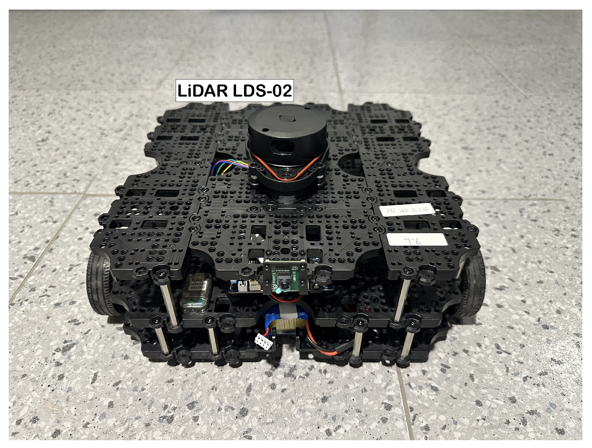
The robotic platform in which the implementation was tested was the TurtleBot3 Waffle Pi by ROBOTIS (ROBOTIS Co., Ltd. 37, Magokjungang 5-ro 1-gil, Gangseo-gu, Seoul, Republic of Korea). It is a ROS-based, programmable robot that can be customized in various ways depending on the assembly of its mechanical parts. The robot is equipped with a 2D LiDAR LDS-02 sensor, a Raspberry Pi4 single board computer (Raspberry Pi Foundation, Hills Road, Cambridge, England, UK), a 32-bit ARM Cortex®-M7 with FPU (216 MHz, 462 DMIPS) MCU (Arm, 110 Fulbourn Road Cambridge, UK), an OpenCR 1.0 board, two DYNAMIXEL XM430-W210-T motors, and a Raspberry Pi Camera Module v2.1 (Raspberry Pi Foundation, Hills Road, Cambridge, England, UK). It has a maximum translational velocity of 0.26 m/s and a maximum rotational velocity of 1.82 rad/s. The robot was assembled and its components were connected following the ROBOTIS e-Manual for the TurtleBot3 Waffle Pi. The setups for both the Raspberry Pi and the OpenCR board were also done following the e-Manual.
The 2D LiDAR LDS-02 sensor in the robot is a 360-degree laser distance sensor used to perceive the environment. It emits a laser and measures its intensity and flight time after being reflected from the object to obtain the distance at which it is located. It has a sampling rate of 2.3 kHz, an operating range from 160 mm to 8000 mm, and an angular resolution of 1
∘, which can vary depending on the scan frequency of the LiDAR. The robot and its LDS-02 LiDAR sensor are shown in
Figure 3.
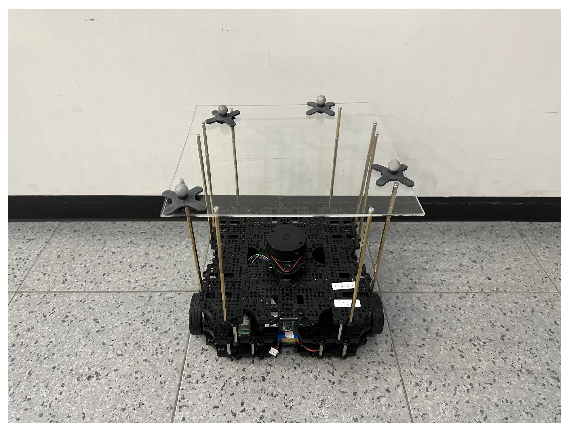
For the MoCap system to be able to provide the location of the robot in the area, four retroreflective markers were attached to the robot. These markers reflect light to the cameras in the MoCap system so their location can be triangulated and shown in the software. The markers must be at a height of 30 centimeters and positioned in an asymmetrical pattern for the system to work accurately when calculating the position of the rigid body, thus an extra platform was attached to the robot for the markers to be at the desired height.
Figure 4 shows the chosen placement of the markers in the TurtleBot3.
3.2. OptiTrack-Motive Motion Capture System
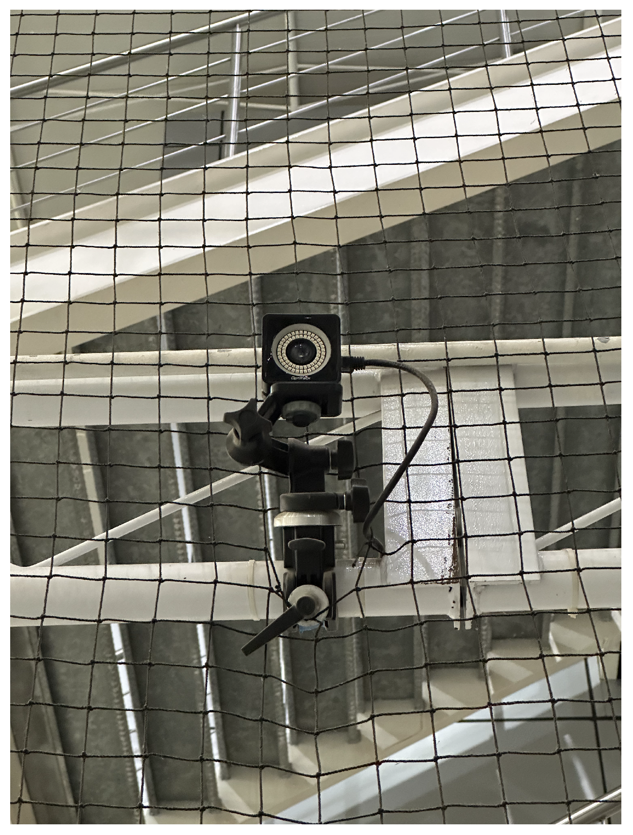
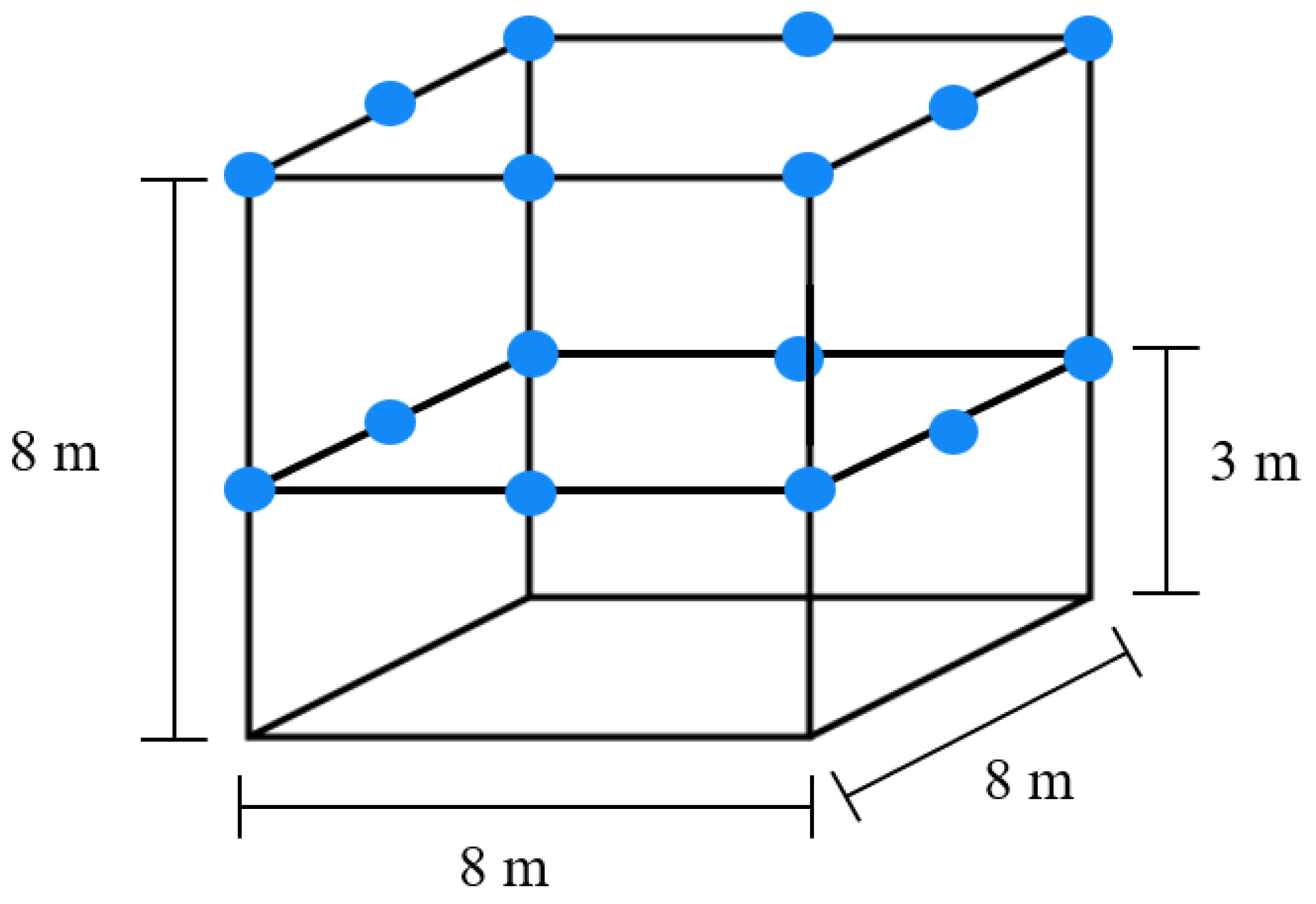
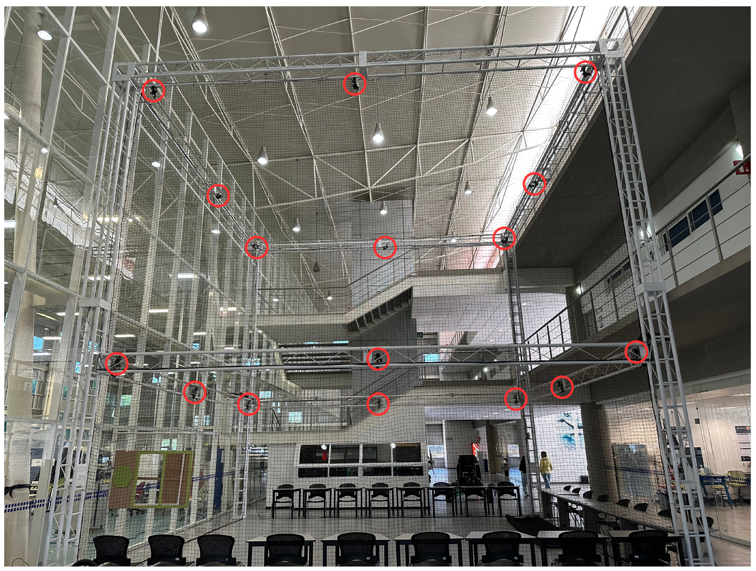
The physical implementation occurred in the OptiTrack-Motive Motion Capture System at Tecnológico de Monterrey Campus Querétaro. It consists of a space measuring 8m x 8m x 8m, enclosed by a net. It contains 16 OptiTrack Prime 13 MoCap cameras by NaturalPoint Inc. (NaturalPoint, 3658 SW Deschutes St, Corvallis, OR, USA), shown in
Figure 5, encircling the space. 8 of the cameras are located at a height of 3 meters from the ground and the other 8 cameras are at a height of 8 meters. The cameras are calibrated and referenced to a point in the center of the arena at a height of 3 meters.
A simple model of the system is shown in
Figure 6, where the blue circles represent the position of each of the 16 cameras. A picture of the MoCap system is shown in
Figure 7, where the cameras are marked with red circles. The cameras provide accurate positioning of markers in a 3D plane through the Motive 2.2 software, which will be used in the implementation for obtaining the robot’s position. Since the robots are located at near-ground height, only the data from the 8 lower cameras was used.
The data obtained from the Motive 2.2 software was migrated to ROS Noetic through a ROS driver developed by Thakker [
33], which is compatible with the NatNet 4.0 protocol that is used by the Motive software. With these data and the data obtained from the 2D LDS-02 LiDAR sensor, the neural network’s performance was tested in the physical environment using the TurtleBot3 Waffle Pi.
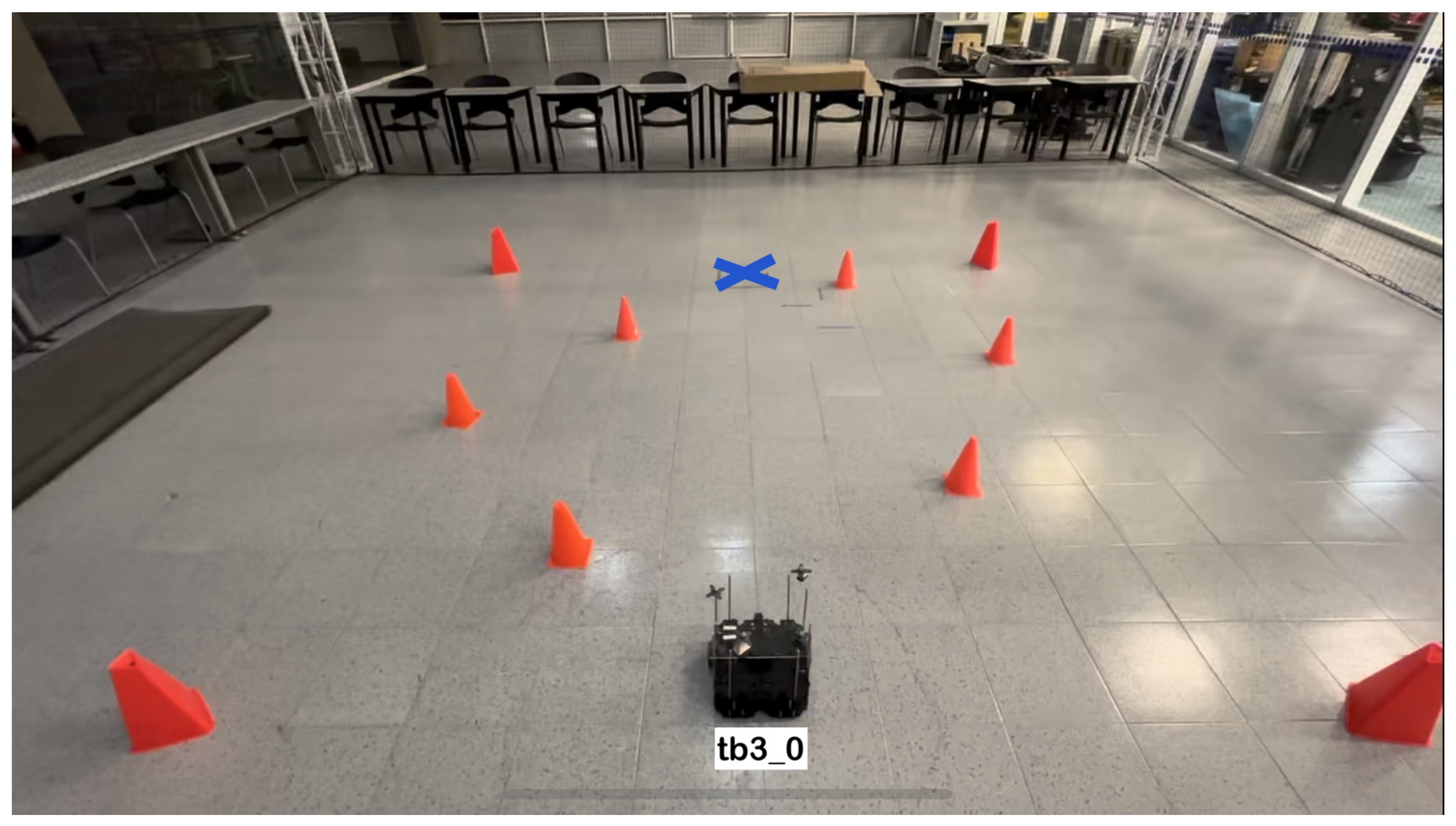
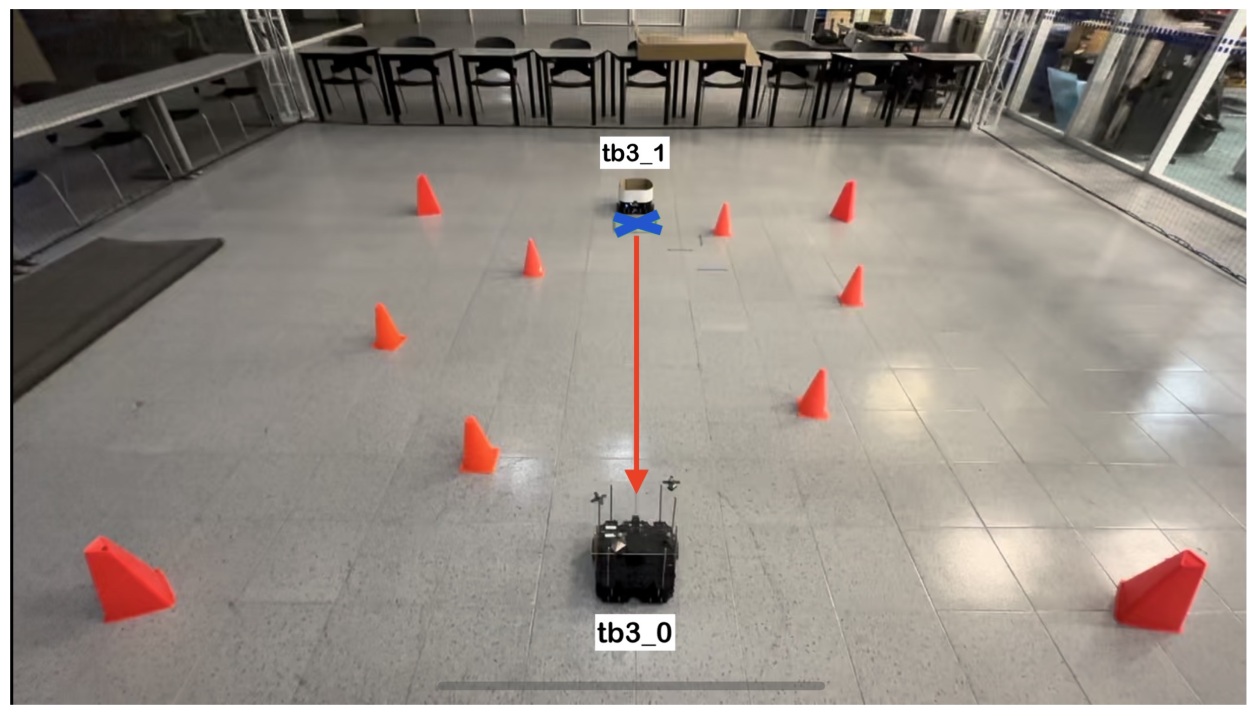
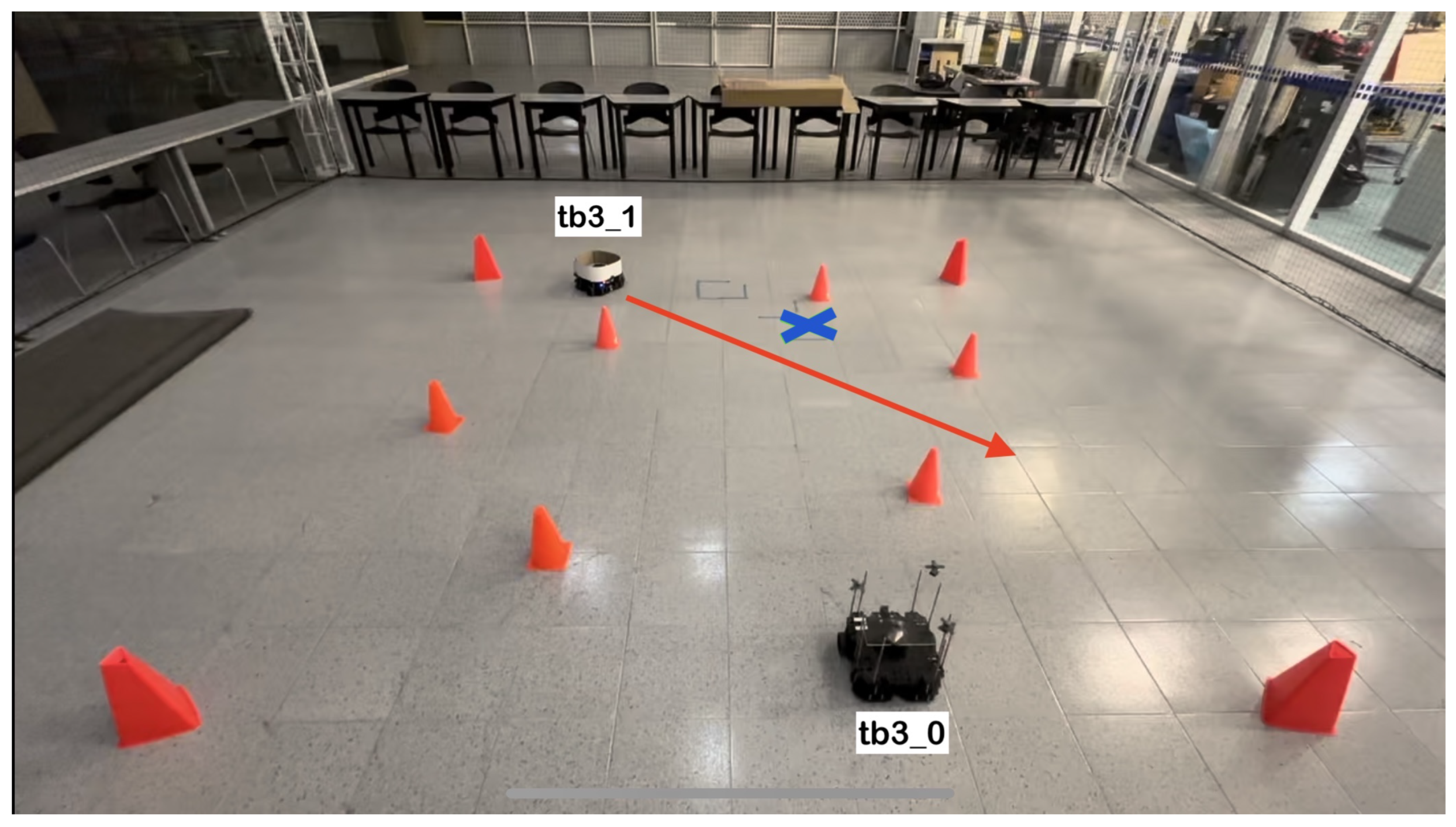
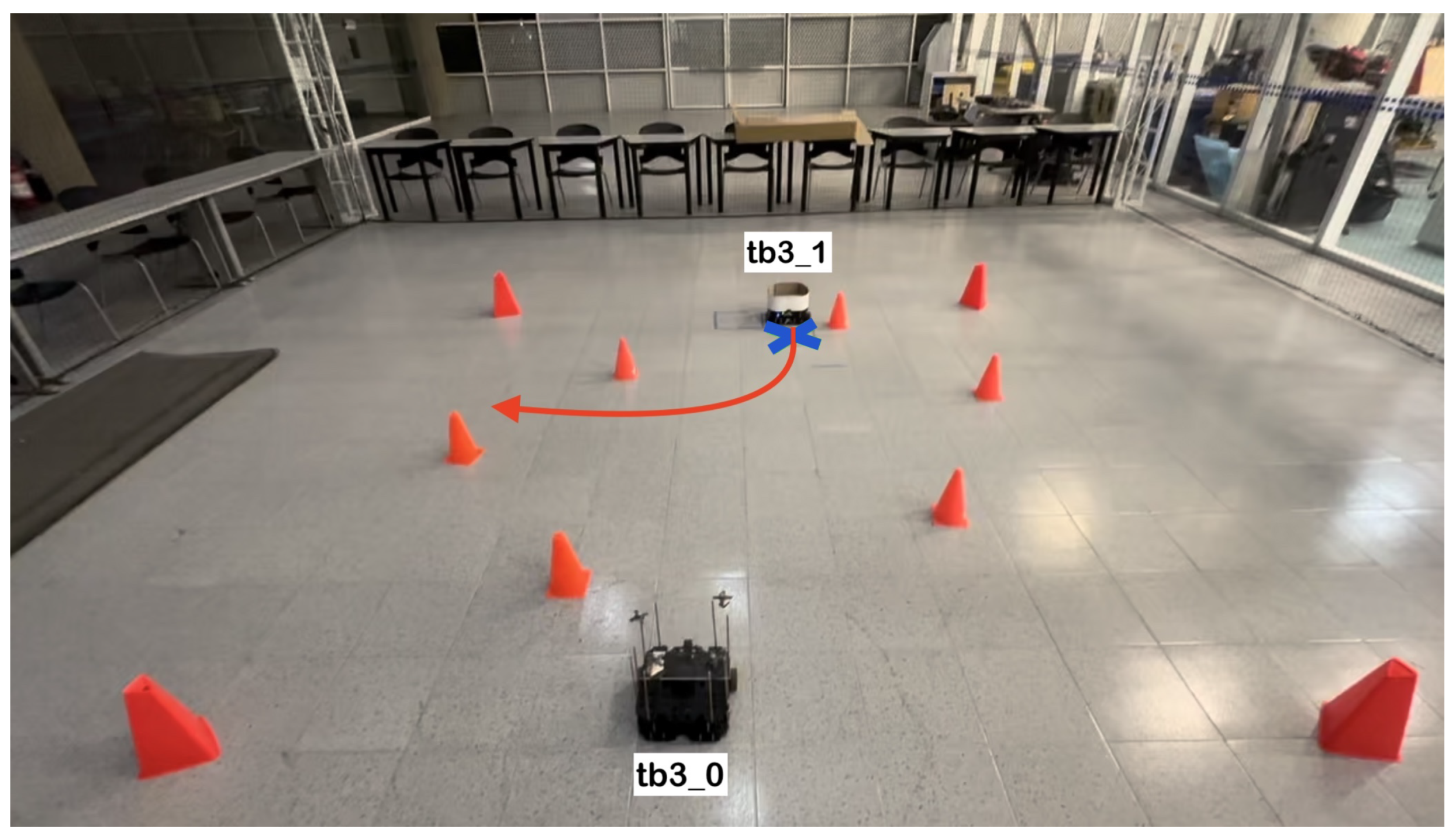
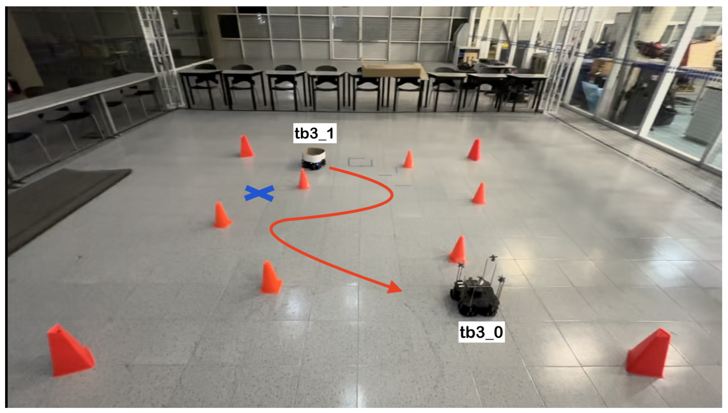
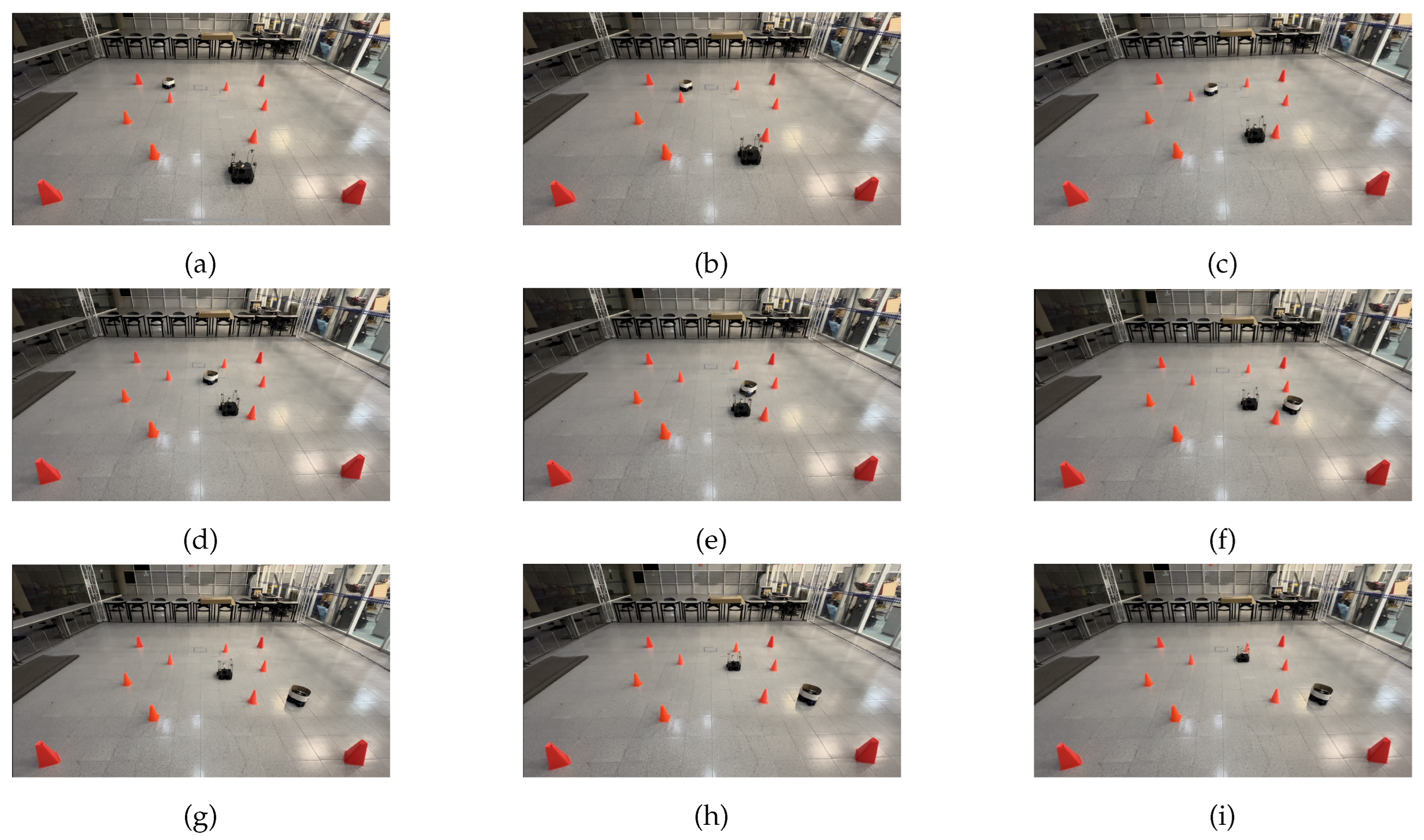
The physical setup inside the MoCap system consisted of six static obstacles simulating a narrow aisle and a dynamic obstacle represented by a TurtleBot3 Waffle Pi with different starting points depending on the training scenario. Five different navigation scenarios for the mobile robot were implemented. These scenarios are shown in
Figure 8,
Figure 9,
Figure 10,
Figure 11 and
Figure 12, with tb3_0 being the mobile robot and tb3_1 being the dynamic obstacle.
3.3. Software
Multiple software tools were required for the implementation of this project. Most of these were run using a Dell G15 5520 computer (Dell Technologies, 1 Dell Way Round Rock, TX, US) running with an Intel Core i7 12700H processor (Intel, 2200 Mission College Blvd, Santa Clara, CA, USA), 16 GB RAM, and an Nvidia GeForce RTX 3060 graphics card (Nvidia, 2788 San Tomas Expy, Santa Clara, CA, USA). The experiments were run using the Ubuntu 20.04 (Ubuntu, 5 Blue Fin Bldg, 110 Southwark St, LDN, UK) Linux distribution.
Using Ubuntu 20.04, ROS Noetic was installed, along with the required packages. It was also necessary to install Python 3.8.10 for writing scripts to control the dynamic obstacle, write to a .csv file, and train, validate, and test the neural network, as well as Keras 2.13.1 for modeling the LSTM network.
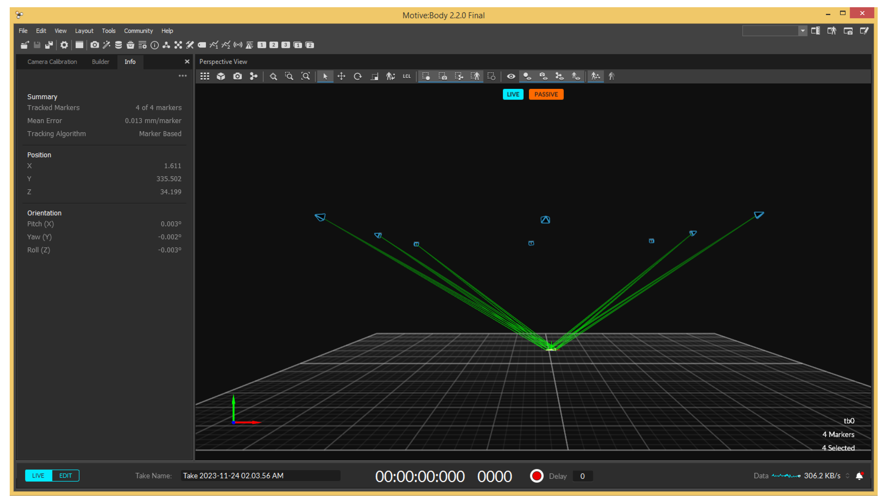
For the motion capture system, an extra computer running the Motive 2.2 software was used. Motive pairs with the OptiTrack cameras in the physical setup to track the motion of retroreflective markers attached to the robot, providing real-time position data with a high level of accuracy. An example of how the software’s interface looks is shown in
Figure 13.
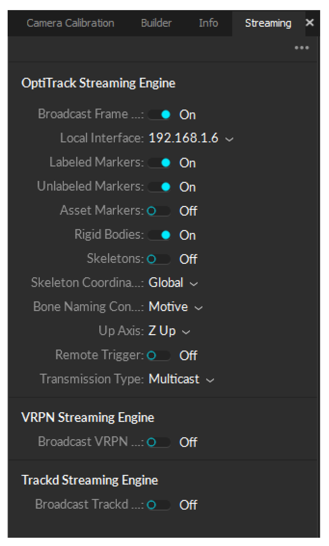
The data obtained from the software was migrated to ROS using the NatNet protocol, which streams live MoCap data across a network shared between the streaming and receiver computers so it can be used for training the neural network. Certain settings must be modified in the streaming pane of the Motive software for the protocol to work correctly. These settings are shown in
Figure 14.
3.4. Data Acquisition
The data used for the neural network’s training consisted of the target point for the robot, the LiDAR sensor’s readings, the robot’s linear and angular velocities, and the robot’s position given by the motion capture system every 0.2 seconds. The LiDAR readings used were those taken every two degrees, spanning the front 180∘ of the robot. Due to the varying sampling rate of the physical LiDAR, the values were filtered using a code that obtains the laser’s readings and organizes them into an array that contains the 90 readings from the front of the robot, and publishes them to a new topic. A ROS node subscribes to the new laser scan topic of the TurtleBot3 LiDAR scan data, the linear and angular velocities of the robot given by the "cmd_vel" topic at each time instance, and the robot’s position given by the MoCap system.
The robot’s position at each time instance was obtained through the Motive 2.2 software. Four retroreflective markers were positioned on the robot in an asymmetric pattern so the cameras could track its position accurately. The position in the x and y axis obtained by the OptiTrack MoCap system was streamed in Motive using the NatNet protocol driver and the data was migrated to ROS, which was then recorded to a .csv file, along with the 90 laser readings, the target point for the robot and the linear and angular velocities of the robot for training the LSTM neural network.
3.5. LSTM Neural Network
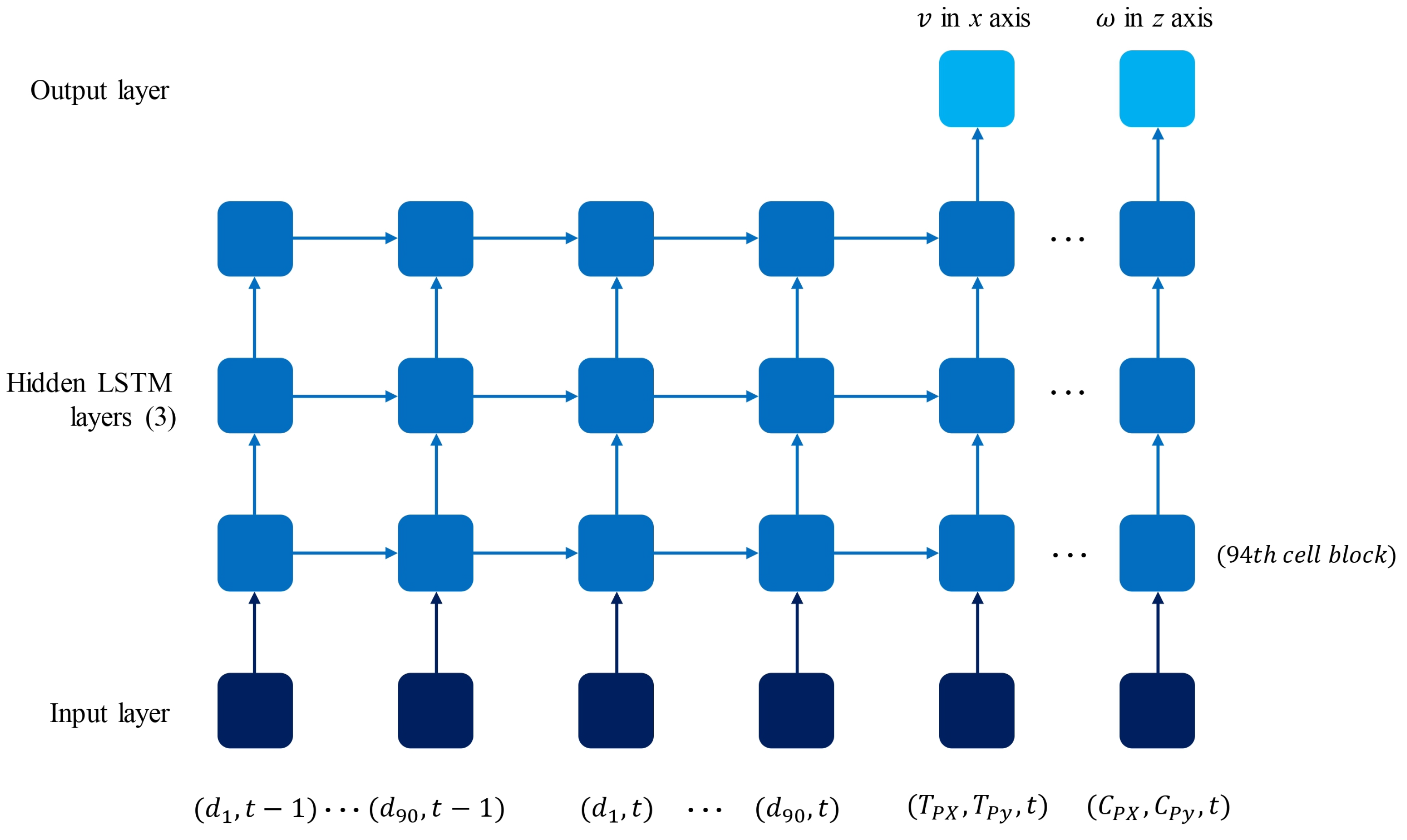
The architecture of the implemented LSTM neural network,
Figure 15, consists of an input layer of 188 blocks that contain 94 features that describe the position of the robot (
), the target location (
), and the data from the laser scan (
), all in timestamp
t, as well as the data from the laser scan in timestamp
. Next, it contains three hidden layers of 94 LSTM cell blocks each. The first two of these layers are set to return a sequence output, meaning they provide an output for each timestep to the layer below. The output layer contains two neurons that return the linear and angular velocity of the mobile robot in
x and
z, respectively. The loss of the network is calculated as the mean squared error, optimized with an Adam model, and trained for 400 epochs with a batch size of 32. The recorded data in .csv format was reshaped using the Keras library to fit the
batch size,
time steps, and
features parameters of the LSTM model, considering the features and the previous time step.
Since the model deals with a large number of trainable parameters, dropout is used as a solution for overfitting. 30% dropout layers were added between the hidden layers. A ROS node, “testing”, subscribes to the laser scan topic and obtains online LiDAR sensor data, publishing it to the twist (velocity) topic with the LSTM model predicted velocities for tb3_0. The
roslaunch tool was used to start three ROS nodes: one with the obstacle controller algorithm, “speed_controller”, one with the LSTM model testing navigation, “testing” [
22], and a third one that obtains the motion capture system’s data so that the navigation of the mobile robot with the proposed model could be tested in the designated area.
4. Results
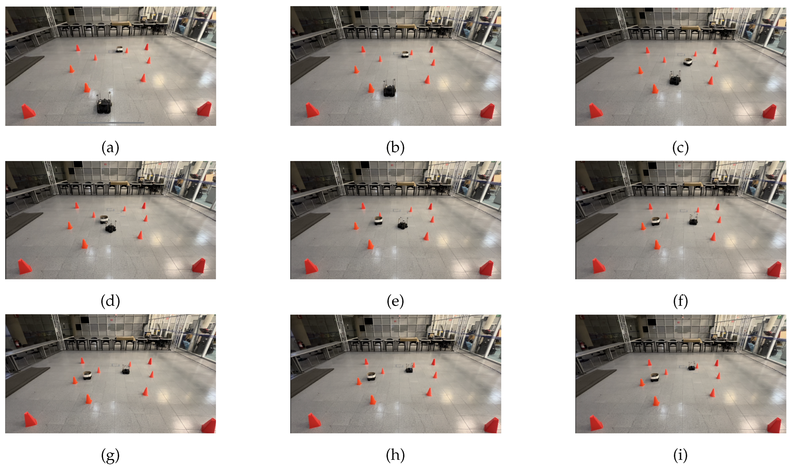
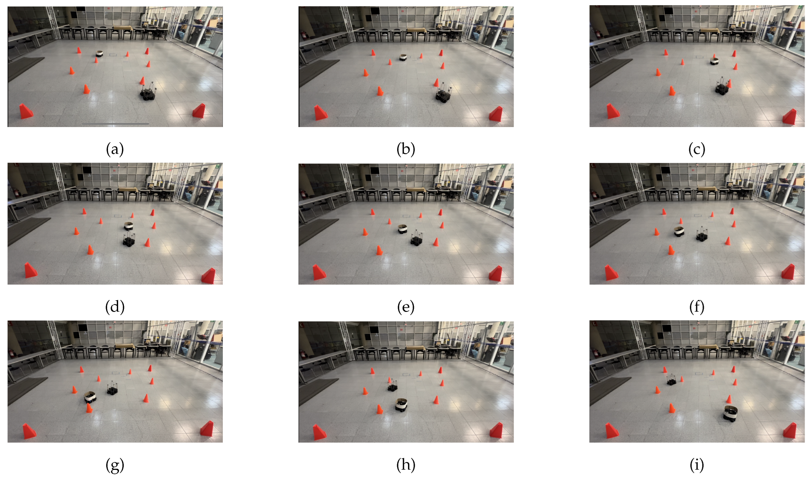
The model was trained using 100 different trajectory examples through five different scenarios, consisting of an instance where there was no dynamic obstacle and another four scenarios with different starting and target points for the mobile robot, as well as different trajectories for the dynamic obstacle in each of them. The first two scenarios analyze what the robot would do when moving through a narrow aisle with no obstacles versus encountering a dynamic obstacle directly in front of it. The other three scenarios study the behavior of the robot when the dynamic obstacle presents more complex trajectories, such as crossing its path diagonally, changing directions suddenly, or following a more complex, curved, zigzag-like path that crosses the robot’s trajectory toward its goal.
The criteria used for determining whether the model was successful in its task are as follows: the mobile robot must reach its target within a 10 cm radius of the original goal point, and it must do so while avoiding collisions with both static and dynamic obstacles. The time it took for the robot to reach its target was also recorded. Each scenario was run through twenty times to ensure the model had enough data for the robot to move autonomously when testing the LSTM neural network.
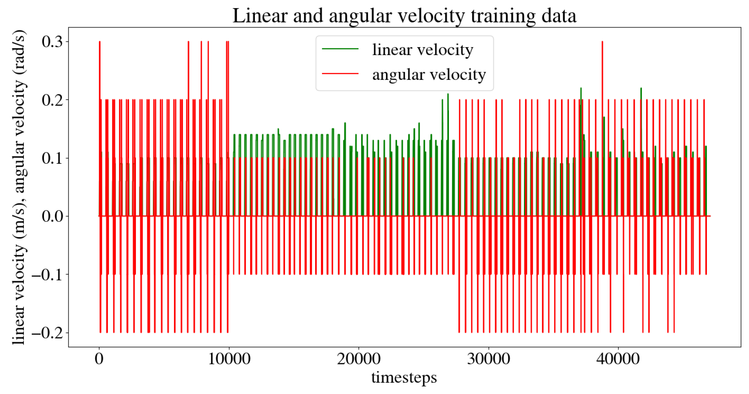
Figure 16 shows the linear and angular velocity commands given by the user during all the training instances for the five trajectories.
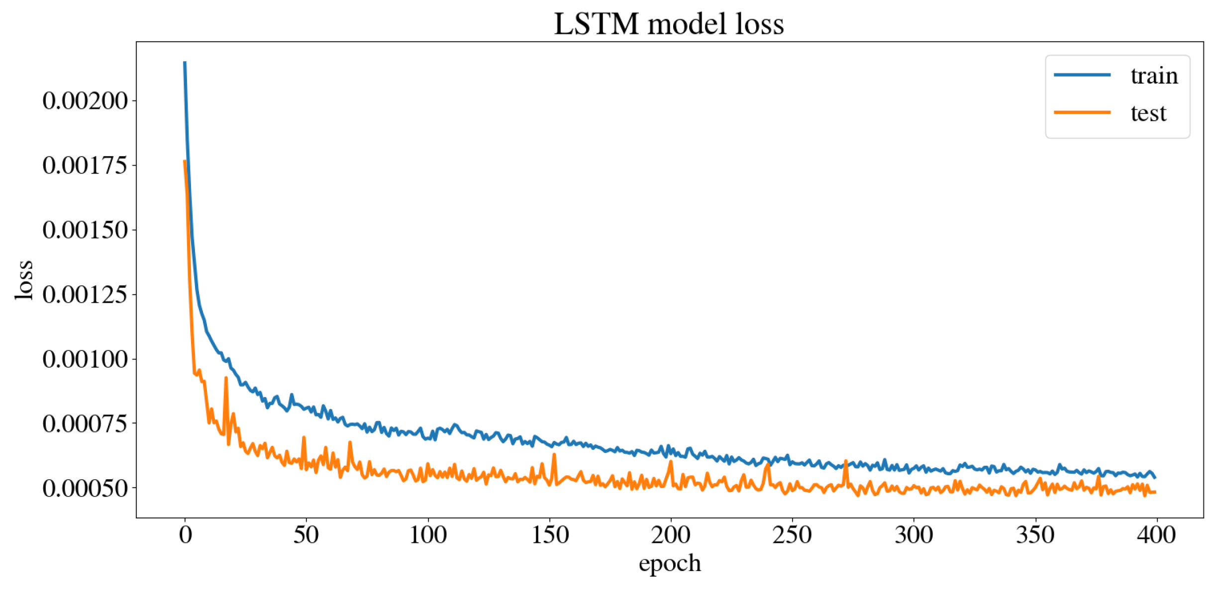
The dataset obtained from the user’s navigation of the five trajectories was split randomly into 80% for the train set and 20% for the test set. The model was trained and validated, obtaining the model train and test loss curve presented in
Figure 17. A Mean Squared Error (MSE) of 0.0003 m/s was obtained for the linear velocity in the
x axis, as well as a MSE of 0.0007 rad/s for the angular velocity in the
z axis, and an accuracy of 98.02%.
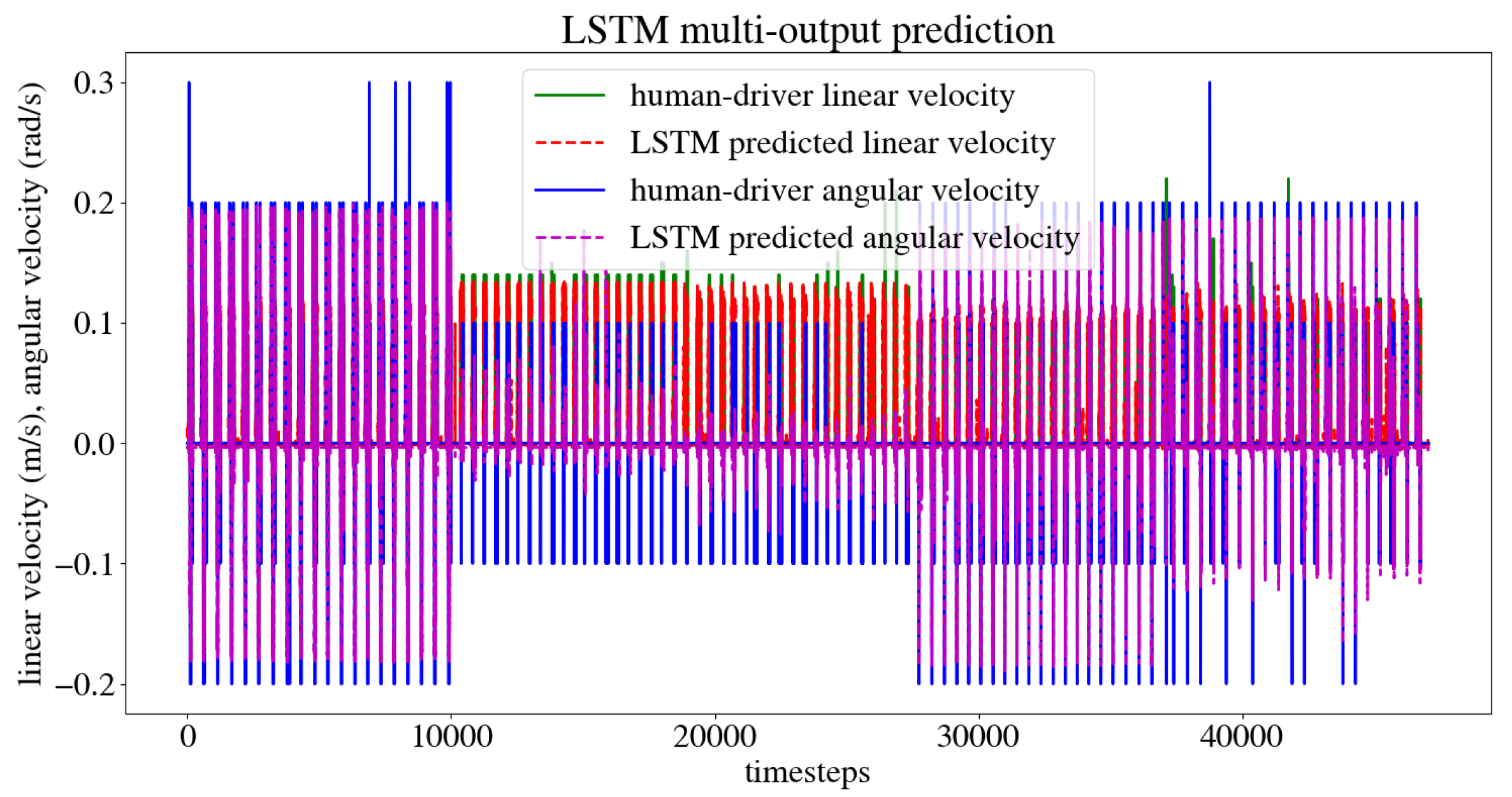
Figure 18 shows the predicted linear and angular velocities for the model, compared to those given by the user during training.
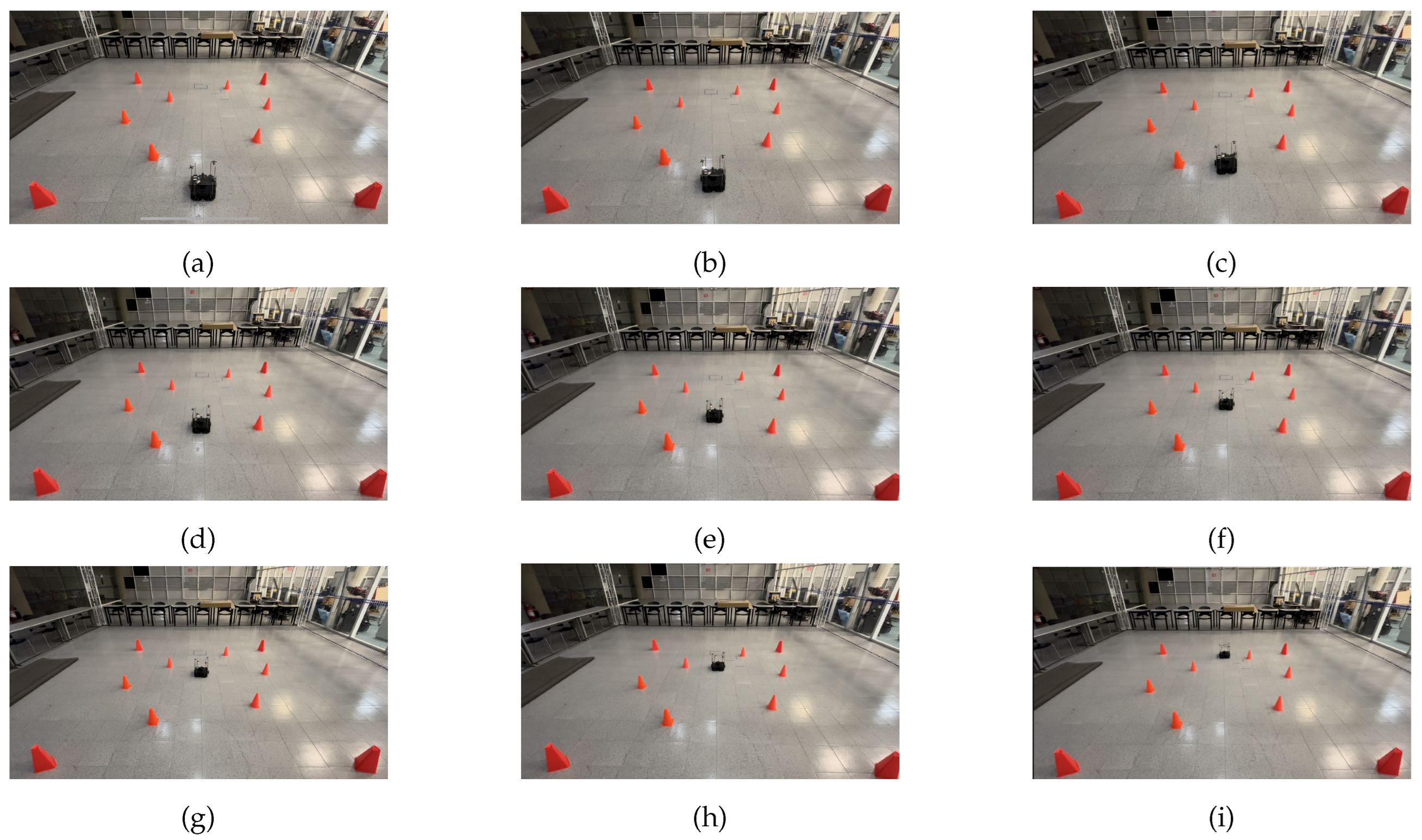
The LSTM model was tested in the same five scenarios. In the first scenario, the target point for the robot is (-0.3, 1.8) and there is no dynamic obstacle, so the robot moves straight ahead towards the target point. The trajectory followed by the robot is shown in
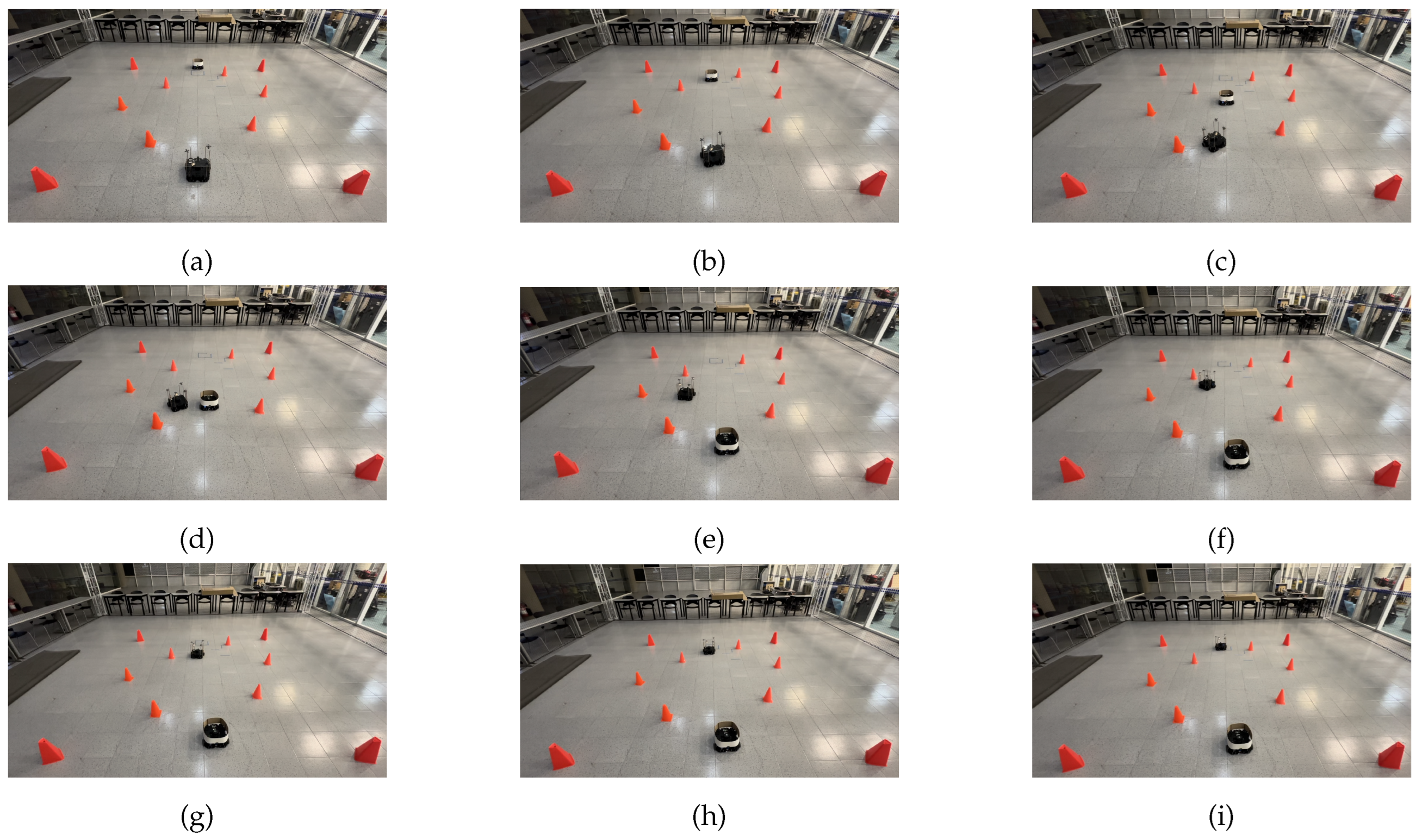
Figure 19. In the second scenario, the target point is still (-0.3, 1.8), however, the dynamic obstacle is placed in front of the robot and follows a linear trajectory, so the robot takes a small curve to avoid the obstacle and get to the target point, as seen in
Figure 20. In the third scenario, the target point for the robot is (0.2, 1.2) and the dynamic obstacle crosses the robot’s path in a diagonal trajectory, forcing the robot to stop and let the obstacle through, continuing its path afterwards. The interaction is shown in
Figure 21.
Figure 22 illustrates the fourth scenario, in which the robot’s target point is (0.0, 1.5) and the dynamic obstacle is placed in front of the robot and follows a curved "L" trajectory, forcing the robot to avoid it. Finally,
Figure 23 shows the fifth scenario. Here, the target point for the robot is (-1.5, 0.8), with the dynamic obstacle following a curved zig-zag-like trajectory that crosses the robot’s path and forces it to stop and let the obstacle pass, continuing its course afterward.
The model was tested multiple times in the same circumstances to ensure that the robot would reach the desired position while avoiding both dynamic and static obstacles in the different scenarios. Each time, the mobile robot reached its target within a 10 cm radius from the original goal point. The obtained results are presented in
Table 1.
As can be seen in
Table 1, the presented model achieved its purpose while meeting the previously set criteria for success. Through numerous runs of the five scenarios in which the mobile robot had to avoid static and dynamic obstacles to reach a goal point, it did so every time it was tested. The target was reached with an error of less than 10 cm while avoiding collisions with the dynamic and static obstacles, even in situations where the mobile robot had to stop, let the dynamic obstacle through, and continue its path afterward, which proves the effectiveness of the proposed method.
5. Conclusions
An approach to dynamic obstacle avoidance based on an LSTM Neural Network was implemented using two TurtleBot3 robots to represent the navigating robot and the dynamic obstacle. The robot navigated through its environment using LiDAR readings taken every 2∘ from the front of the robot in a range from 0∘ to 180∘, and its position was obtained using a MoCap system. The robot was given 100 navigating examples through five different scenarios, which were recorded in a .csv file that included the 90 readings from the robot’s LiDAR, the target point, the robot’s position in the x and y axis obtained from the MoCap system, and the robot’s linear and angular velocities in each time instance. The LSTM network was trained using this data. The training results showed an accuracy of 98.02% for the model’s trajectory prediction, as well as a MSE of 0.0003 m/s for the linear velocity in the x axis, and a MSE of 0.0007 rad/s for the angular velocity in the z axis.
The model was tested multiple times, studying its ability to reach the desired goal in each of the five scenarios, with different and complex trajectories for the dynamic obstacle. In each experiment, the robot reached the target point while avoiding collision with the dynamic obstacle, either by changing the angle of its trajectory or by stopping, letting the dynamic obstacle through, and then continuing on its path. The physical implementation of an LSTM neural network model proved to be successful in allowing a robot to navigate from a starting point to a target point while avoiding a dynamic obstacle in five different scenarios.
Future work with the model includes implementing the algorithm in a less controlled scenario, using robotic vision for obtaining the robot’s position in different time instances instead of the MoCap system. Other scenarios could also be explored, such as having the velocity of the dynamic obstacle vary, implementing multiple dynamic obstacles, and adding more training scenarios so the model is more robust.
Author Contributions
Conceptualization, E.M.-T., A.G.-E. and J.A.E.C.; methodology, E.M.-T., A.G.-E. and J.A.E.C.; software, E.M.-T.; validation, E.M.-T.; formal analysis, E.M.-T., A.G.-E. and J.A.E.C.; investigation, E.M.-T.; resources, J.A.E.C.; data curation, E.M.-T.; writing—original draft preparation, E.M.-T.; writing—review and editing, E.M.-T., A.G.-E., J.A.E.C., J.A.C.-C. and A.M.-L.; visualization, E.M.-T.; supervision, A.G.-E. and J.A.E.C.; project administration, J.A.E.C. and A.G.-E.; funding acquisition, A.G.-E. All authors have read and agreed to the published version of the manuscript.
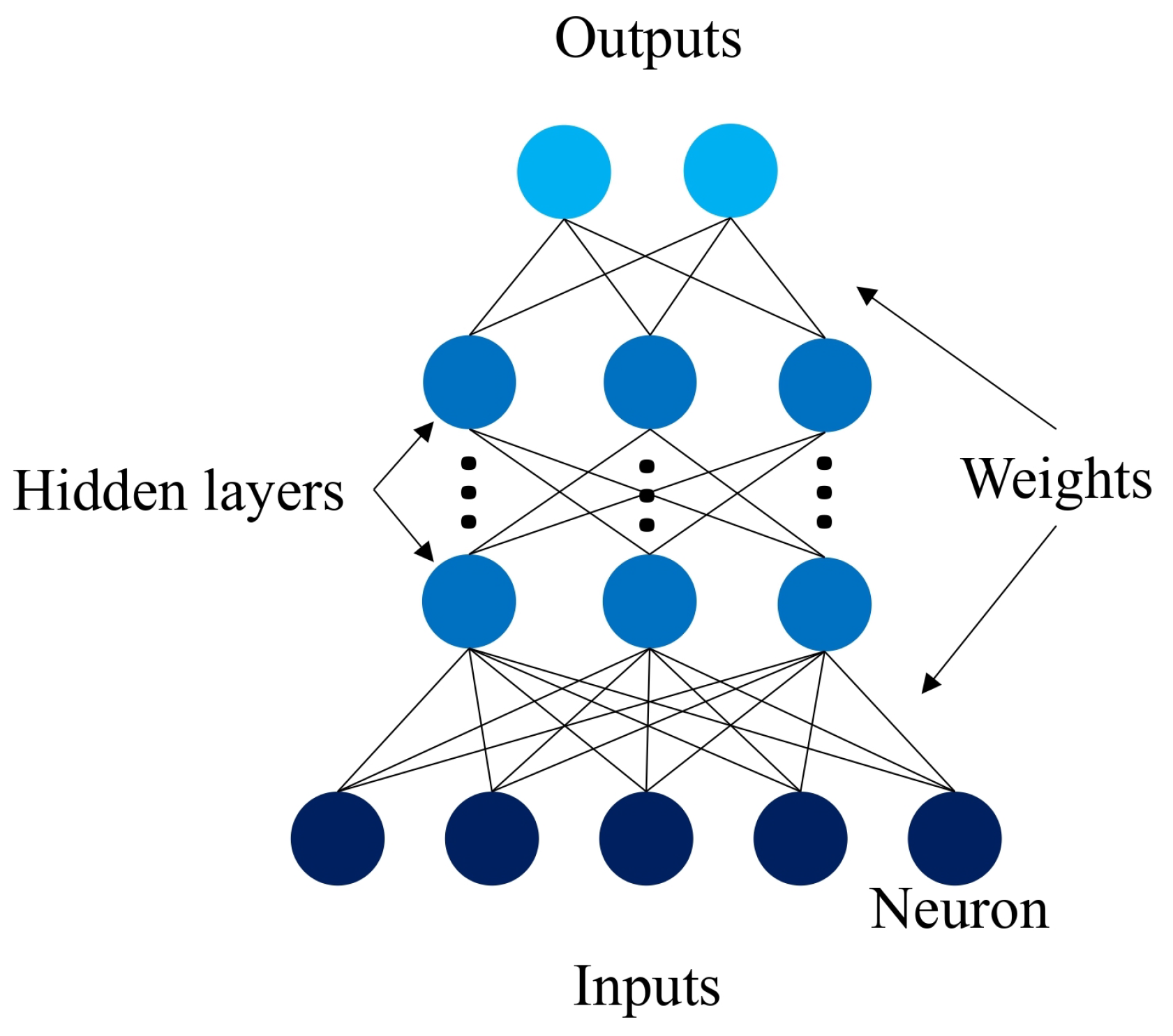
Figure 1.
Neural network model.
Figure 1.
Neural network model.
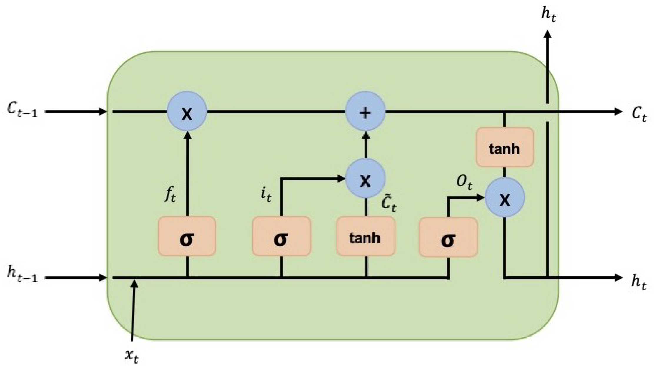
Figure 2.
LSTM cell block diagram.
Figure 2.
LSTM cell block diagram.
Figure 3.
TurtleBot3 Waffle Pi with LiDAR sensor.
Figure 3.
TurtleBot3 Waffle Pi with LiDAR sensor.
Figure 4.
Placement of four retroreflective markers on a TurtleBot3 for obtaining the robot’s position in the MoCap system.
Figure 4.
Placement of four retroreflective markers on a TurtleBot3 for obtaining the robot’s position in the MoCap system.
Figure 5.
OptiTrack Prime 13 camera from the OptiTrack-Motive Motion Capture system.
Figure 5.
OptiTrack Prime 13 camera from the OptiTrack-Motive Motion Capture system.
Figure 6.
OptiTrack-Motive Motion Capture system model.
Figure 6.
OptiTrack-Motive Motion Capture system model.
Figure 7.
Optitrack-Motive Motion Capture system with the cameras highlighted by red circles.
Figure 7.
Optitrack-Motive Motion Capture system with the cameras highlighted by red circles.
Figure 8.
First training scenario. The goal point (-0.3, 1.8) is represented with a blue X mark. There is no dynamic obstacle.
Figure 8.
First training scenario. The goal point (-0.3, 1.8) is represented with a blue X mark. There is no dynamic obstacle.
Figure 9.
Second training scenario. The goal point (-0.3, 1.8) is represented with a blue X mark. The dynamic obstacle follows a straight path toward the robot, shown with a red arrow.
Figure 9.
Second training scenario. The goal point (-0.3, 1.8) is represented with a blue X mark. The dynamic obstacle follows a straight path toward the robot, shown with a red arrow.
Figure 10.
Third training scenario. The goal point (0.2, 1.2) is represented with a blue X mark. The dynamic obstacle follows a diagonal path crossing in front of the robot, shown with a red arrow.
Figure 10.
Third training scenario. The goal point (0.2, 1.2) is represented with a blue X mark. The dynamic obstacle follows a diagonal path crossing in front of the robot, shown with a red arrow.
Figure 11.
Fourth training scenario. The goal point (0.0, 1.5) is represented with a blue X mark. The dynamic obstacle follows a curved path that crosses in front of the robot, shown with a red arrow.
Figure 11.
Fourth training scenario. The goal point (0.0, 1.5) is represented with a blue X mark. The dynamic obstacle follows a curved path that crosses in front of the robot, shown with a red arrow.
Figure 12.
Fifth training scenario. The goal point (-1.5, 0.8) is represented with a blue X mark. The dynamic obstacle follows a curved, zigzag-like path, shown with a red arrow.
Figure 12.
Fifth training scenario. The goal point (-1.5, 0.8) is represented with a blue X mark. The dynamic obstacle follows a curved, zigzag-like path, shown with a red arrow.
Figure 13.
Motive 2.2’s interface showing the robot as a rigid body.
Figure 13.
Motive 2.2’s interface showing the robot as a rigid body.
Figure 14.
Streaming settings in Motive for migrating data using NatNet protocol.
Figure 14.
Streaming settings in Motive for migrating data using NatNet protocol.
Figure 15.
LSTM model architecture with data inputs and outputs.
Figure 15.
LSTM model architecture with data inputs and outputs.
Figure 16.
Linear and angular velocity commands given by the user during training.
Figure 16.
Linear and angular velocity commands given by the user during training.
Figure 17.
Model train and test loss curves.
Figure 17.
Model train and test loss curves.
Figure 18.
Linear and angular predicted velocities versus user-trained velocities.
Figure 18.
Linear and angular predicted velocities versus user-trained velocities.
Figure 19.
Scenario 1: The target point for the robot is (-0.3, 1.8). There is no dynamic obstacle. (a) shows the starting point of the robot, (b)-(h) show the trajectory that it followed and (i) shows the robot at its goal.
Figure 19.
Scenario 1: The target point for the robot is (-0.3, 1.8). There is no dynamic obstacle. (a) shows the starting point of the robot, (b)-(h) show the trajectory that it followed and (i) shows the robot at its goal.
Figure 20.
Scenario 2: The target point for the robot is (-0.3, 1.8). The dynamic obstacle travels in a straight line toward the robot. (a) shows the starting point of the mobile robot and dynamic obstacle, (b)-(h) show the trajectory followed by both and (i) shows the mobile robot at its goal, as well as the dynamic obstacle at its ending point.
Figure 21.
Scenario 3: The target point for the robot is (0.2, 1.2). The dynamic obstacle crosses the robot’s path in a diagonal trajectory. (a) shows the starting point of the mobile robot and dynamic obstacle, (b)-(h) present the trajectory followed by both, and (i) shows the mobile robot at its goal, as well as the dynamic obstacle at its ending point.
Figure 22.
Scenario 4: The target point for the robot is (0.0, 1.5). The dynamic obstacle follows a curved trajectory that crosses the robot’s path. (a) shows the starting point of the mobile robot and dynamic obstacle, (b)-(h) show the trajectory followed by both and (i) shows the mobile robot at its goal, as well as the dynamic obstacle at its ending point.
Figure 23.
Scenario 5: The target point for the robot is (-1.5, 0.8). The dynamic obstacle follows a curved zig-zag trajectory, crossing the robot’s path. (a) shows the starting point of the mobile robot and dynamic obstacle, (b)-(h) show the trajectory followed by both and (i) shows the mobile robot at its goal, as well as the dynamic obstacle at its ending point.
Table 1.
Experimental results from testing the model on five different situations.
Table 1.
Experimental results from testing the model on five different situations.
| Scenario |
Time |
Dynamic obstacle collision |
Static obstacle collision |
| Scenario 1 |
| Goal point (-0.3, 1.8) |
27s |
No |
No |
| Scenario 2 |
| Goal point (-0.3, 1.8) |
38s |
No |
No |
| Scenario 3 |
| Goal point (0.2, 1.2) |
28s |
No |
No |
| Scenario 4 |
| Goal point (0.0, 1.5) |
34s |
No |
No |
| Scenario 5 |
| Goal point (-1.5, 0.8) |
40s |
No |
No |
