Preprint
Article

Selection of the Value of Power Distance Exponent for Mapping with the Inverse Distance Weighting Method - Application in Subsurface Porosity Mapping, Northern Croatia Neogene

Altmetrics

Downloads

52

Views

19

Comments

0

A peer-reviewed article of this preprint also exists.

This version is not peer-reviewed

Submitted:

25 April 2024

Posted:

26 April 2024

You are already at the latest version

Alerts
Abstract
The correct selection of the value of p is a complex and iterative procedure that requires experience in the interpretation of the obtained interpolated maps. Inverse Distance Weighting is a method applied to the porosities of the K and L hydrocarbon reservoirs, discovered in the Neogene (Lower Pontian) subsurface sandstones in the northern Croatia (Pannonian Basin System). They represent small and large data samples. Also a standard statistical analysis of the data was made, followed by the qualitative-quantitative analysis of the maps, based on the selection of different values of the power distance exponent (p-value) for the K and L reservoirs maps. According to the qualitative analysis, for a small data set, p-value could be set on 1 or 2 giving the most optimal result, while for a large data set, a p value of 3 and 4 could be applied. By quantitative analysis, for the case of small data p=2 is recommended, resulting in a root mean square error value of 0.03458, a mean absolute error of 0.02013 and a median absolute deviation of 0.00546. Oppositely, a p-value of 3 and 4 is selected as appropriate for a large data set, with root mean square errors of 0.02435 and 0.02437, mean square errors of 0.01582 and 0.01509 and median absolute deviations 0.00896 and 0.00444. Eventually for a small data set, it is recommended to use a p-value of 2, and for a large data set, a p-value of 3 or 4.
Keywords: 
Subject: Environmental and Earth Sciences  -   Other

1. Introduction

Inverse Distance Weighting (IDW) is an interpolation method that is widely used in geosciences. The method is applied to small and large input data sets. Various authors have applied IDW during different mappings of variables: mapping the distribution of a nickel deposit [1], geomorphology [2], estimated copper, molybdenum, gold and silver with respect to lithogeochemical data in the Kahang porphyry deposit in Central Iran [3], modeling of ionospheric time delay [4], spatial distribution maps of groundwater [5], spatial distribution of groundwater pollution maps [6], mapping of gold deposits based on drilled shallow wells [7], soil salinity mapping in the Mirzaabad District, Syrdarya Province [8], and the estimation of tin resources [9]. The estimated value of the IDW variable is calculated using the following formula: [10,11,12]:
z I D W = z 1 d 1 p + z 2 d 2 p + z n d n p 1 d 1 p + 1 d 2 p + 1 d n p
where:
  • ZIDW  estimated value,
  • d1…dn  distance between estimated value and known value 1…n,
  • p      power distance exponent,
  • z1…zn       known values at locations 1…n.
The mapping results are greatly influenced by the power distance exponent (p), this is clear because it represents the exponent of a value that is inversely reciprocal to the known "hard" data, as can be seen from formula 1. This is why it is important to choose p correctly so that the obtained interpolated maps are usable and mathematically based. Both the size (small or large) and the nature of the input data set should be considered when choosing p. The wrong selection of p can lead to asymmetry in the resulting interpolation maps, which should be avoided. In this paper, the selection of p will be analyzed considering the quantitative (sample size, cross-validation) and qualitative (visual inspection and interpretation) aspects of the obtained interpolation maps.

2. Materials and Methods

For the analysis of the value of p, it is necessary to take into account the material and applied methods. The material data are contained in the values of the porosity of the reservoirs K and L. In addition to the previously described IDW, the coefficient of interquartile deviation, root mean square error, mean absolute error and median absolute deviation calculations were applied for analysis.

2.1. Coefficient of Interquartile Deviation

Coefficient of interquartile deviation (VQ) is a measure of incomplete dispersion of a data set, and is defined as [13,14]:
V Q = Q 3 Q 1 Q 1 + Q 3
where:
  • VQ coefficient of interquartile deviation,
  • Q1 the value of the lower (first) quartile of the sample,
  • Q3 the value of the upper (third) quartile of the sample.
The value of the coefficient is between 0 and 1, the condition for its application is that all input data are positive values (>0). The dispersion of the data is smaller the closer VQ is to 0, and relatively larger the closer VQ is to 1.

2.2. Root Mean Square Error (RMSE)

Cross-validation is a numerical value obtained as the difference of the square of the measured and estimated data values. Mean square error is calculated according to [15,16]:
M S E = 1 n i = 1 n ( S V P ) i 2
where:
  • MSE  - Mean Square Error value,
  • n     - number of known values,
  • SV     - measured value of point „i“,
  • P        - estimated value of point „i“,
  • i      - ith point.
It quantitatively expresses the quality of the interpolation map, the lower the RMSE value, the higher the acceptability of the interpolated map. During the interpolation process while changing various parameters, RMSE is a corrective for interpolation maps because it reduces the space for gross errors. Root Mean Square Error value is calculated according to [17,18]:
R M S E = M S E
where:
  • RMSE  - Root Mean Square Error value,
  • MSE     - Mean Square Error value.
RMSE due to the root function of the error itself means that larger errors will contribute less in absolute terms. This is very important when analyzing a large input data set.

2.3. Mean Absolute Error (MAE)

Mean Absolute Error is a measure of error calculated as the difference between the measured and estimated sample values. The formula for calculating MAE is [19,20]:
M A E = 1 n i = 1 n S V P i
where:
  • MAE - Mean Absolute Error,
  • n     - number of known values,
  • SV     - measured value of point „i“,
  • P        - estimated value of point „i“,
  • i      - ith point.
As can be seen from expression 5, the MAE represents a comparison between the "firm" data and the estimated data. The MAE method is sensitive to extreme values within the input data set.

2.4. Median Absolute Deviation (MAD)

Median absolute deviation is the median value of the difference between the estimated value and the value of the "solid" data. MAD is calculated according to the following equation [21,22]:
M A D = m e d i a n S V P i
where:
  • MAD - Median Absolute Deviation,
  • SV    - measured value of point „i“,
  • P      - estimated value of point „i“,
  • i     - ith point.

3. Geographic Location, Geological Settings and Raw Data of Analysed Reservoirs

Research fields “A” and “B” are located within the Sava Depression, in the Croatian part of the Pannonian Basin System (CPBS) (see Figure 1). Sediments filling the Sava Depression started already in Early Neogene (Otnangian), and in this study Lower Pontian reservoir rocks (reservoirs K and L) belonging to the Kloštar-Ivanić Formation are analyzed (see geological column in Figure 1). These are mainly well-sorted arenitic sandstones, becoming fine-grained and loose toward the top of the Široko Polje Formation, and intercalated with marl intervals. Reservoir rocks are well-lithified sandstones, with an average thickness of 20-150 m. Isolator rocks are gray to gray-brown marls, moderately lithified, appearing in 30-150 m thick intervals between sandstones.
The Lower Pontian sediments (also known informally by their older name Abichi deposits, after characteristic fossil shell Paradacna abichi) extended across the entire Sava Depression, but in the most western part can be represented with the Kloštar-Ivanić Marls (as lateral equivalent of the Kloštar-Ivanić Formation) or locally as the Brezine or Graberje Marl. The analysed sandstones (as part of the Poljana Sandstones) are the result of periodically activated turbidites and are deposited in the deepest part of the depression. The rest had been filled with marls, occasionally silty ones.
The most important petrophysical parameter during reservoir analysis is porosity. Data on the porosity of the deposits K and L were obtained by analyzing cores from a well or by interpreting logging diagrams. The porosity value for the K reservoir was obtained from 19 wells, while for the L reservoir it was obtained from 25 wells, and they are considered "solid" data, i.e. the original data during various analyses. Basic statistical data on the porosity of the reservoirs K and L are shown in Table 1. It is obvious that the quality and resolution of the measuring devices and the transformation of indirect signals into values had significant limitations, especially in the reservoir K, where numerous wells have the same average porosity value for sandstone. However, it is a common limitation that must be overridden using the most appropriate interpolation algorithm, and handled with the same values as some kind of "clusters", even if they are not located in their own neighborhood.

4. Results and discussion

The choice of reservoir was made considering the size of the input data set. The size of the input data set is taken according to the authors [26], according to which the reservoir K belongs to a small data set, while the reservoir L belongs to a large data set. The values of the coefficient of interquartile deviation for the K and L reservoirs are presented in Table 2.
According to Table 2, the VQ value for the K reservoir is 0.013, while for the L reservoir it is 0.054. According to these values, the porosity of these reservoirs is significantly dispersed. This was to be expected due to the nature of the input data and the method of obtaining it. Due to the high economic cost of obtaining data, the input data set is in most cases very dispersed. Precisely because of the large depressiveness of the data, the IDW method was applied for mapping the reservoirs K and L.

4.1. Qualitative Analysis of Maps

A qualitative analysis of interpolated maps implies a visual inspection of the map and the existence of the following visual mapping results: bulls-eye (circular), butterfly (ellipsoidal) and mosaic [27]. During the visual analysis of the maps, maps with a value of p=0 were not analyzed, because according to equation 1, in that case the solution of the equation would be same. The results of the mapping of reservoirs K and L using the IDW method for p values of 1,2,3 and 4 are shown in Figure 2 and Figure 3.
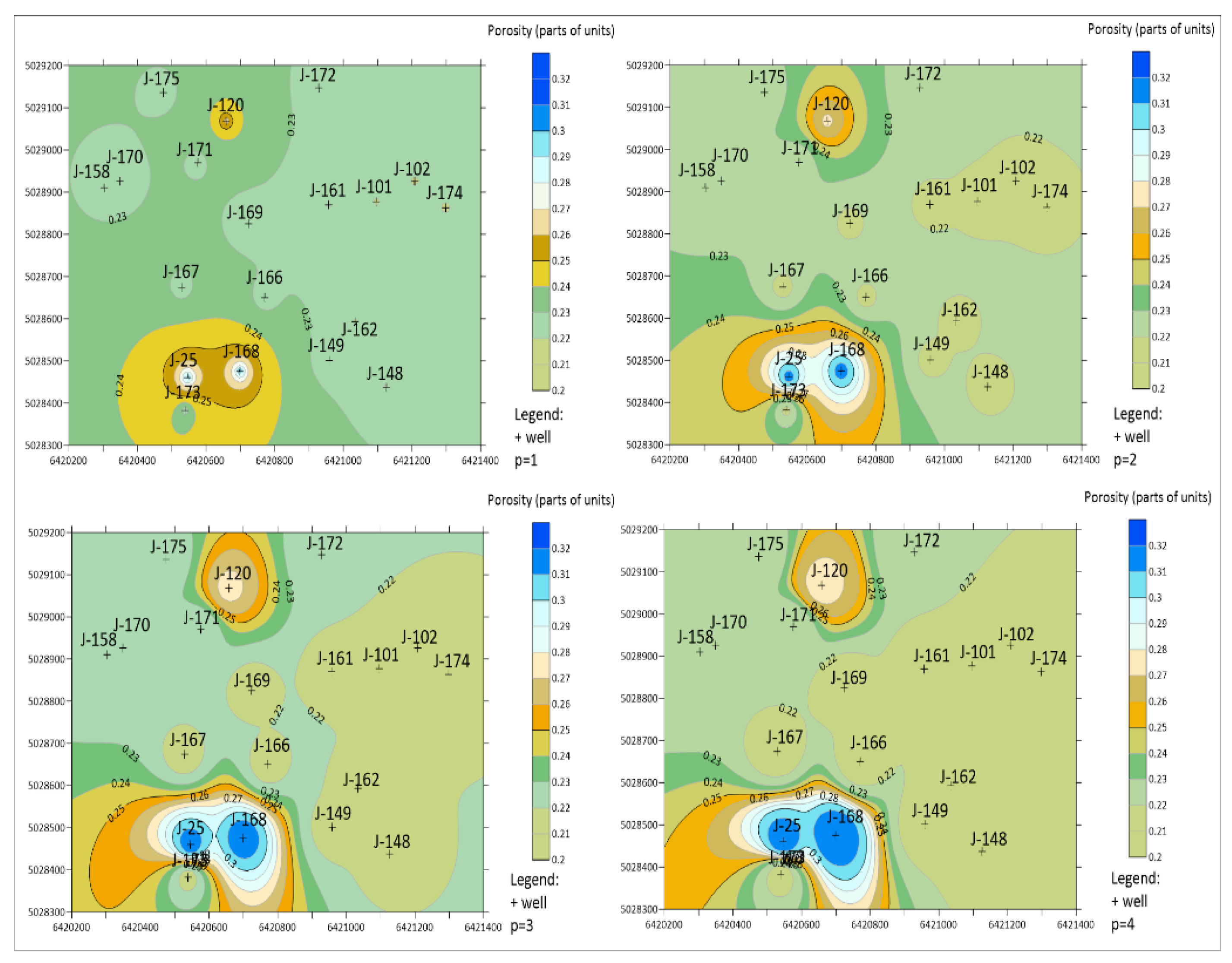
In the case of reservoir K (see Figure 2), with an increasing value of p, a pronounced bulls-eye effect (p=1, p=2) and butterfly effect (p=3, p=4) appears. At higher values, such as J-25, J-168, etc. regardless of the change in the value of p, the effect was not removed, but the changes were detected as a pronounced bulls-eye effect into a butterfly effect. With an increase in the value of p, there was no mosaic effect, which is positive. The transition zones are different in all cases of a change of p, the clearest transition zone is seen in the case of p=2 and does not have such a pronounced asymmetric value change, as in other cases. Also, with a p value of 2, it can be applied to reduce the number of bulls-eyes to only extreme values of the input data. In cases where bulls-eye and butterfly effects are expressed on the maps, from a visual point of view, interpolated maps with a bulls-eye effect are preferred. With the bulls-eye effect, the value is evenly distributed around the point data, while with the butterfly effect, there is an ellipsoidal surface around the point data, which due to the appearance can encompass space, which is not realistic. Therefore, on the example of the interpolated map obtained in Figure 2, i.e. in the case of a small data set, the value of p is 1 and 2 when using the IDW method.
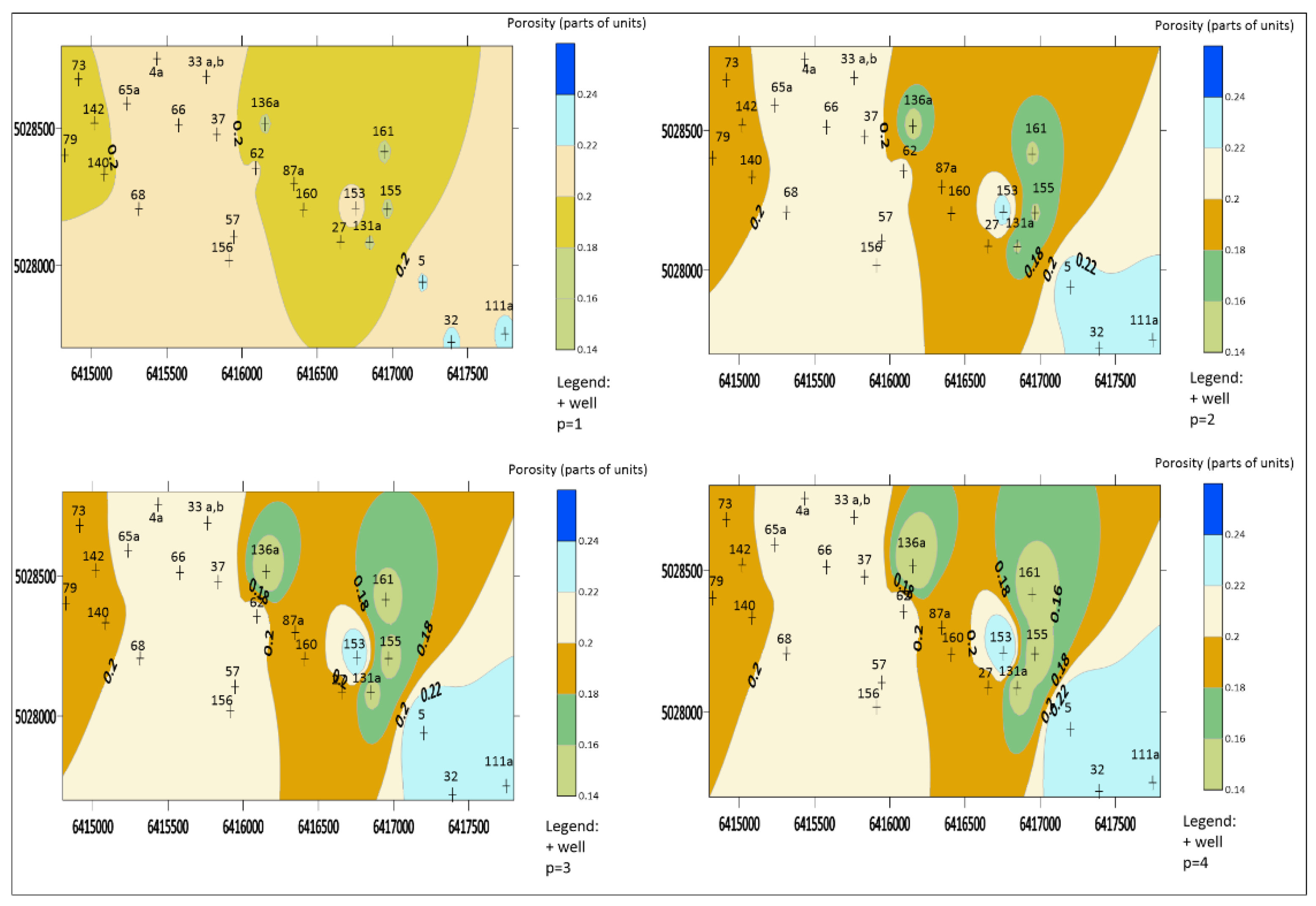
The porosity map of the reservoir L (see Figure 3) for all cases of p values have a pronounced butterfly effect. As the value of p increases in this case, the bulls-eye and mosaic effect are not present, which is evident from the obtained interpolation map. The reason for this is that it is a large data set, because the input data set is sufficient to perform a satisfactory interpolation in the given area. The transition area between different input data values is clearer when interpolating with p values of 3 and 4. For p values of 3 and 4, it is very clear that the reservoir L is tectonically very clearly divided and the stability of transition zones is conditioned by the values of individual data with neighboring ones, which can be seen in the eastern parts of the interpolated maps as a rather asymmetric area of porosity values. Considering the transition zones and the inclusion of input data in the interpolated maps, for a large data set, the recommendation from the visual inspection of the maps is to use p values of 3 and 4 when applying the IDW method.

4.2. Quantitative Analysis of Maps

The quantitative analysis is expressed by the numerical value of RMSE, MAE and MAD, the results of which are shown in Table 3 for the K and L reservoirs.
The values of RMSE and MAE for the reservoir K increase as the value of the coefficient p increases, while the value of MAD varies. The RMSE values are 0.00104-0.00155, and the values of MAE are 0.01700-0.02319, which shows continuous but almost linear growth. The MAD value is not linear and takes on values 0.00360-0.00734. According to the RMSE, MAE and MAD values, the smallest value of the interpolated porosity map of the reservoir K with p values of 1 and 2. Unlike reservoir K, the RMSE, MAE and MAD values for reservoir L are not in a linear relationship. RMSE values are 0.0263-0.02470, MAE values are 0.01924-0.01490, and MAD values are 0.00869-0.00343. As can be seen from Table 3, for a value of p of 1, it has the highest value, while for values of p of 3 and 4, it has the lowest value for the interpolated maps of the porosity of the reservoir L. According to the quantitative methods and the RMSE, MAE and MAD values, for a small sample, the optimal value of p is 1 and 2, while for a large sample, the optimal value of p is 3 and 4.

4.3. Qualitative-Quantitative Approach in Selection of p-Value

Most of the authors who analyzed the p value in the IDW method took a data set that belongs to a large data set. Moreover, IDW is one of the most applied interpolation methods overall in many sciences that deal with spatial data, e.g. in mining [28] or soil mapping for military application [29]. However, the selection of p-value as standard for any scientific field is a very hard, if not impossible task, and often depends not only on discipline, but also on the geographical location of data. Such a geographically locked analysis is presented here as an example of subsurface geological mapping in the northern Croatia Neogene sandstones, and geological background defined what is considered as "small" and "large" data sets (in some other disciplines and locations, such definition could be totally different).
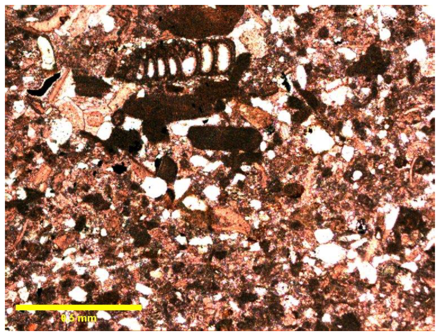
Both data sets had been considered for a comprehensive p-value analysis, including both qualitative and quantitative analyses, shown for the hydrocarbon reservoirs K and L of Lower Pontian age. Looking only of numerical values of the RMSE, MAE and MAD could lead to the conclusion that only the lowest values are criteria for the "best" p-value. Especially because Neogene northern Croatian sandstones are often of very heterogeneous porosity, including primary and secondary ones as the result of numerous events of compaction, relaxing, dissolutions and fracturing, as shown in Figure 4.
It is obligatory to also visually inspect the porosity maps and eliminate ones where some impossible subsurface shapes exist (like butterfly or too strong bulls-eye effects) or known faults with distorted isoporosity lines of continuity. Using both criteria, it is clear that for a small data set, the optimal p is 2, while for a large data set, the optimal value is 3 and 4. This is a recommendation for the application of the IDW method in the northern Croatia Lower Pontian sandstones porosity mapping, while it is definitely recommended for other sciences to analyze the input data set and perform a quantitative-qualitative analysis.

5. Conclusions

Data sets in geosciences are dispersed and in most cases are presented in the form of limited data sets. Two of them had been analysed for the porosity data of the K and L hydrocarbon reservoirs of the Neogene age in the northern Croatia. The main results of the qualitative-quantitative analysis are:
-
For a small data set, it is recommended to use a p-value of 2, because in this case, the butterfly effect is eliminated, and the RMSE value of 0.00119, MAE value of 0.02103, and MAD value of 0.00546 are smaller with respect to larger p values.
-
The p value of 3 and 4 is optimal in the case of a large data set, because the transition zones are clear and the input data set is included, and this is confirmed by the following values: RMSE (0.02435, 0.02437), MAE (0.01582, 0.01509) and MAD (0.00896, 0.00444).
-
Data dispersion in the case of a small and large data set is present, but when changing the value of p, it gradually affects the obtained interpolation maps.
-
The IDW method in both cases gave usable results and due to the similar lithologies in most of the Sava Depression (northern Croatia), it is recommended to apply the IDW method with p-values between 2-4, depending on the size of the analysed porosity data set.

Author Contributions

Conceptualization, J.I., U.B and T.M.; methodology J.I., U.B and T.M.; validation, J.I., U.B and T.M; investigation, J.I.; writing—original draft preparation, J.I. and U.B.; writing—review and editing, J.I., U.B and T.M.; visualization, J.I. All authors have read and agreed to the published version of the manuscript.

Funding

Please add: This research received no external funding.

Data Availability Statement

Not applicable.

Acknowledgments

The authors thank the anonymous reviewers and editors for their generous and constructive comments that have improved this paper. This research was partially carried out in the projects “Mathematical researching in geology VIII” (led by T. Malvić).

Conflicts of Interest

The authors declare no conflicts of interest.

References

  1. Bartier, P. M.; Keller, C. P. Multivariate interpolation to incorporate thematic surface data using inverse distance weighting (IDW). Computers & Geosciences 1996, 22(7), 795–799.
  2. Gossel, W., Falkenhagen, M. Line-Geometry-Based Inverse Distance Weighted Interpolation (L-IDW): Geoscientific Case Studies. In Proceedings of the Mathematics of Planet Earth. Springer, Berlin, Germany, 08 October 2013. [CrossRef]
  3. Karami, R.; Afzal, P. Estimation of Elemental Distributions by Combining Artificial Neural Network and Inverse Distance Weighted (IDW) Based on Lithogeochemical Data in Kahang Porphry Deposit, Central Iran. Universal Journal of Geoscience 2015, 3, 59 – 65. [CrossRef]
  4. Srinivas, V. S.; Sarma, A. D.; Achanta, H. K. Modeling of Ionospheric Time Delay Using Anisotropic IDW with Jackknife Technique. IEEE Transactions on Geoscience and Remote Sensing 2016, 54, 513–519. [Google Scholar] [CrossRef]
  5. Mircovski, V.; Gicevski, B.; Dimov, G. Hydrochemical characteristics of the groundwaters in Prilep’s part of Pelagonia valley – Republic of Macedonia. Rudarsko-geološko-Naftni Zbornik 2018, 33, 111–119. [Google Scholar] [CrossRef]
  6. Maliqi, E.; Idrizi, B.; Penev, P. Compilation of groundwater monitoring maps for the Mitrovica region in Kosova. Geoscience and Remote Sensing 2019, 2, 41–55. [Google Scholar] [CrossRef]
  7. Liming S., Yingqi, W.; Hong C.; Jun, Y.; Jianzhang, X. Improved Fast Adaptive IDW Interpolation Algorithm based on the Borehole Data Sample Characteristic and Its Application. In Proceedings of the 3rd International Conference on Data Mining, Communications and Information Technology, Beijing, China, 24–26 May 2019. [CrossRef]
  8. Pulatov, A.; Khamidov, A; Akhmatov, D.; Pulatov, B.; Vasenev, V. Soil salinity mapping by different interpolation methods in Mirzaabad district, Syrdarya Province. In Proceedings of the International Scientific Conference Construction Mechanics, Hydraulics and Water Resources Engineering, Tashkent, Uzbekistan, 23-25 April 2020. [CrossRef]
  9. Gonzales, R.; Rahardi, M. R. G.; Octova, A. Estimation of tin resources using Inverse distance weighted (IDW) and nearest neighbor point (NNP) methods in Bangka Tengah district, Bangka Belitung islands province. Georest 2023, 2, 2–7. [Google Scholar] [CrossRef]
  10. Achilleos, G.A. The Inverse Distance Weighted interpolation method and error propagation mechanism – creating a DEM from an analogue topographical map, Journal of Spatial Science 2011, 56, 283-304. [CrossRef]
  11. Maleika, W. Inverse distance weighting method optimization in the process of digital terrain model creation based on data collected from a multibeam echosounder. Appl Geomat 2020, 12, 397–407. [Google Scholar] [CrossRef]
  12. Liu, Z.; Zhang, Z.; Zhou, C.; Ming, W.; Du, Z. An Adaptive Inverse-Distance Weighting Interpolation Method Considering Spatial Differentiation in 3D Geological Modeling. Geosciences 2021, 11, 51. [Google Scholar] [CrossRef]
  13. Yadav, S.K.; Singh, S.; Gupta, R. Measures of Dispersion. In: Biomedical Statistics; Springer, Singapore, 2019; pp. 59-71. [CrossRef]
  14. Botta-Dukát, Z. Quartile coefficient of variation is more robust than CV for traits calculated as a ratio. Sci Rep 2023, 13, 4671. [Google Scholar] [CrossRef] [PubMed]
  15. Browne, M. W. Cross-Validation Methods. Journal of Mathematical Psychology 2000, 44(1), 108–132. [Google Scholar] [CrossRef] [PubMed]
  16. Rodríguez, J.D.; Martínez, A.P.; Lozano, J.A. Sensitivity Analysis of k-Fold Cross Validation in Prediction Error Estimation. IEEE Transactions on Pattern Analysis and Machine Intelligence 2010, 32, 569–575. [Google Scholar] [CrossRef] [PubMed]
  17. Chai, T.; Draxler, R.R. (2014). Root mean square error (RMSE) or mean absolute error (MAE)?– Arguments against avoiding RMSE in the literature. Geoscientific Model Development 2014, 7, 1247-1250. [CrossRef]
  18. Ćalasan, M.; Abdel Aleem, S. H. E.; Zobaa, A. F. On the root mean square error (RMSE) calculation for parameter estimation of photovoltaic models: A novel exact analytical solution based on Lambert W function. Energy Conversion and Management 2020, 210, 112716. [Google Scholar] [CrossRef]
  19. Willmott, C. J.; Kenji, M. Advantages of the mean absolute error (MAE) over the root mean square error (RMSE) in assessing average model performance. Climate Research 2005, 30, 79–82. [Google Scholar] [CrossRef]
  20. Hodson, T. O. Root-mean-square error (RMSE) or mean absolute error (MAE): when to use them or not. Geoscientific Model Development 2022, 15. [Google Scholar] [CrossRef]
  21. Pham-Gia, T.; Hung, T.L. The mean and median absolute deviations. Mathematical and Computer Modelling 2001, 34, 921–936. [Google Scholar] [CrossRef]
  22. Elamir, E. Mean Absolute Deviation about Median as a Tool of Explanatory Data Analysis. International Journal of Recent Research and Applied Studies 2012, 11, 517–523. [Google Scholar]
  23. Ivšinović, J.; Malvić, T. Application of the radial basis function interpolation method in selected reservoirs of the Croatian part of the Pannonian Basin System. Mining of mineral deposits 2020, 14, 37–42. [Google Scholar] [CrossRef]
  24. Ivšinović, J.; Pimenta Dinis, M.A.; Malvić, T.; Pleše, D. (2021) Application of the bootstrap method in low-sampled Upper Miocene sandstone hydrocarbon reservoirs: a case study. Energy Sources, Part A: Recovery, Utilization, and Environmental Effects 2021, 41 1-15. [CrossRef]
  25. Malvić, T.; Ivšinović, J.; Velić, J.; Rajić, R. Kriging with a Small Number of Data Points Supported by Jack-Knifing, a Case Study in the Sava Depression (Northern Croatia). Geosciences 2019, 9, 36. [Google Scholar] [CrossRef]
  26. Malvić, T.; Ivšinović, J.; Velić, J.; Rajić, R. Interpolation of Small Datasets in the Sandstone Hydrocarbon Reservoirs, Case Study of the Sava Depression, Croatia. Geosciences 2019, 9, 201. [Google Scholar] [CrossRef]
  27. Ivšinović, J.; Malvić, T. Comparison of mapping efficiency for small datasets using inverse distance weighting vs. moving average, Northern Croatia Miocene hydrocarbon reservoir. Geologija 2022, 65, 47–57. [Google Scholar] [CrossRef]
  28. Rezaei, M., & Fallahi, S. (2023). Block model optimization and resource estimation of the Angouran Mine by transferring the exploratory data from the local coordinate system to the UTM. Rudarsko-geološko-Naftni Zbornik, 38(3), 1–17. [CrossRef]
  29. Heštera, H., Pahernik, M., Kovačević Zelić, B., & Maurić Maljković, M. (2023). The Unified Soil Classification System Mapping of the Pannonian Basin in Croatia using Multinominal Logistic Regression and Inverse Distance Weighting Interpolation. Rudarsko-geološko-Naftni Zbornik, 38(3), 147–159. [CrossRef]
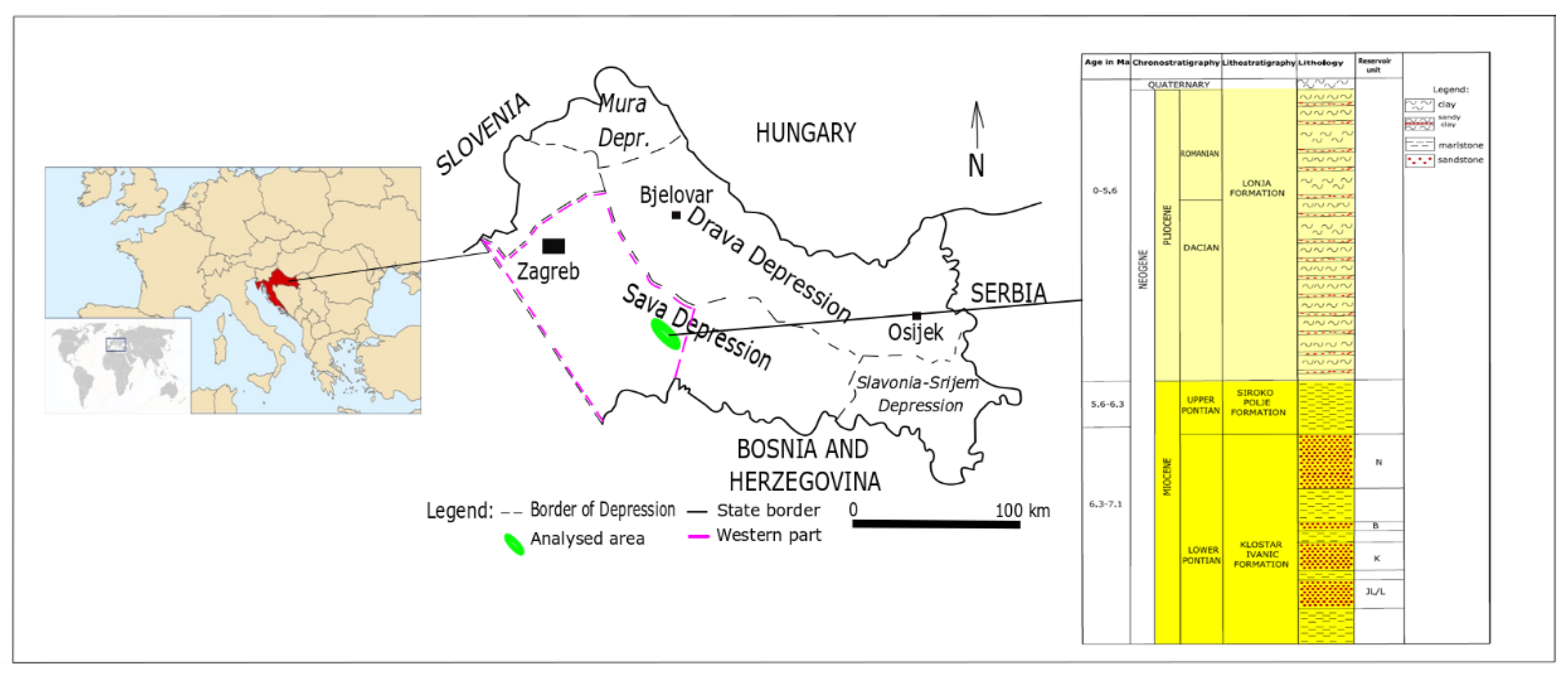
Figure 1. Geographical position and geological column of the research fields A and B within the Sava Depression, modified after [23,24].
Preprints 104820 g001
Figure 2. Maps of the porosity of the K reservoir obtained by the IDW method for values of p=1,2,3,4.
Preprints 104820 g002
Figure 3. Maps of the porosity of the L reservoir obtained by the IDW method for values of p=1,2,3,4.
Preprints 104820 g003
Figure 4. A photomicrograph of the typical Middle Miocene calcarenite from northern Croatia.
Preprints 104820 g004
Table 1. Porosity data for reservoirs K and L [25].
Reservoir K
Well X Y Porosity (part of units) Age
J-101 6421096 5028877 0.217 Lower Pontian
J-120 6420658 5029068 0.272 Lower Pontian
J-161 6420957 5028870 0.217 Lower Pontian
J-162 6421034 5028593 0.217 Lower Pontian
J-167 6420529 5028674 0.217 Lower Pontian
J-168 6420699 5028475 0.315 Lower Pontian
J-169 6420724 5028825 0.217 Lower Pontian
J-170 6420349 5028926 0.223 Lower Pontian
J-174 6421298 5028863 0.217 Lower Pontian
J-175 6420475 5029136 0.223 Lower Pontian
J-158 6420303 5028910 0.223 Lower Pontian
J-171 6420576 5028970 0.223 Lower Pontian
J-172 6420928 5029147 0.223 Lower Pontian
J-102 6421208 5028926 0.217 Lower Pontian
J-148 6421126 5028437 0.217 Lower Pontian
J-149 6420959 5028501 0.217 Lower Pontian
J-166 6420771 5028650 0.217 Lower Pontian
J-25 6420546 5028460 0.315 Lower Pontian
J-173 6420539 5028382 0.217 Lower Pontian
Reservoir L
Well X Y Porosity (part of units) Age
L-111a 6417748 5027750 0.239 Lower Pontian
L-131a 6416847 5028084 0.156 Lower Pontian
L-136a 6416153 5028515 0.145 Lower Pontian
L-140 6415085 5028332 0.192 Lower Pontian
L-142 6415019 5028519 0.186 Lower Pontian
L-32 6416755 5028208 0.239 Lower Pontian
L-155 6416967 5028205 0.156 Lower Pontian
L-156 6415912 5028018 0.206 Lower Pontian
L-160 6416410 5028203 0.197 Lower Pontian
L-161 6416946 5028415 0.156 Lower Pontian
L-27 6416655 5028086 0.197 Lower Pontian
L-153 6417390 5027720 0.239 Lower Pontian
L-33a 6415763 5028687 0.214 Lower Pontian
L-33b 6415763 5028687 0.214 Lower Pontian
L-37 6415834 5028477 0.214 Lower Pontian
L-4a 6415435 5028754 0.214 Lower Pontian
L-5 6417200 5027939 0.239 Lower Pontian
L-57 6415946 5028104 0.206 Lower Pontian
L-62 6416091 5028355 0.206 Lower Pontian
L-65a 6415235 5028590 0.214 Lower Pontian
L-66 6415579 5028512 0.214 Lower Pontian
L-68 6415315 5028206 0.214 Lower Pontian
L-140 6414912 5028679 0.192 Lower Pontian
L-79 6414821 5028402 0.195 Lower Pontian
L-87alfa 6416347 5028297 0.197 Lower Pontian
Table 2. Values of the coefficient of interquartile deviation for the K and L reservoirs.
Reservoir Q1 Q3 VQ
K 0.217 0.223 0.013
L 0.192 0.214 0.054
Table 3. RMSE, MAE and MAD value for different values of p for the K and L reservoirs.
Reservoir p RMSE MAE MAD
K 1 0.03228 0.01700 0.00360
2 0.03458 0.02013 0.00546
3 0.03677 0.02196 0.00383
4 0.03780 0.02276 0.00667
5 0.03839 0.02319 0.00734
L 1 0.02632 0.01924 0.00869
2 0.02505 0.01735 0.01012
3 0.02435 0.01582 0.00896
4 0.02437 0.01509 0.00444
5 0.02470 0.01490 0.00343
Disclaimer/Publisher’s Note: The statements, opinions and data contained in all publications are solely those of the individual author(s) and contributor(s) and not of MDPI and/or the editor(s). MDPI and/or the editor(s) disclaim responsibility for any injury to people or property resulting from any ideas, methods, instructions or products referred to in the content.
Copyright: This open access article is published under a Creative Commons CC BY 4.0 license, which permit the free download, distribution, and reuse, provided that the author and preprint are cited in any reuse.
Prerpints.org logo

Preprints.org is a free preprint server supported by MDPI in Basel, Switzerland.

Subscribe

© 2024 MDPI (Basel, Switzerland) unless otherwise stated