Preprint

Article

EEG-Visual Multiclass Classification Based on a Channel Selection, MNE Algorithm and Deep Network Architectures

Altmetrics

Downloads

135

Views

114

Comments

A peer-reviewed article of this preprint also exists.

Tat’y Mwata-Velu^*,

Erik Zamora^*,

Juan Irving Vasquez-Gomez

Jose Ruiz-Pinales

Juan Humberto Sossa Azuela

Tat’y Mwata-Velu^*,

Erik Zamora^*,

Juan Irving Vasquez-Gomez

Jose Ruiz-Pinales

Juan Humberto Sossa Azuela

This version is not peer-reviewed

Submitted:

26 April 2024

Posted:

28 April 2024

You are already at the latest version

Alerts

Abstract

This work addresses the challenge of EEG visual multiclass classification into 40 classes for Brain-Computer interface applications, by using deep learning architectures. The visual multiclass classification approach offers BCI applications a significant advantage, since it allows the supervision of more than one BCI interaction, considering that each class label supervises a BCI task. However, because of the nonlinearity and nonstationarity of EEG signals, performing multiclassifiers based on EEG features remains a significant challenge for BCI systems. In the present work, mutual information-based discriminant channel selection and Minimum-Norm Estimate algorithms are implemented to select discriminant channels and enhance EEG data. Hence, deep EEGNet and Convolutional-recurrent neural networks are implemented separately to classify EEG data of image visualization into 40 labels. By using the k-fold cross-validation approach, average classification accuracies of 94.8% and 89.8% were obtained by implementing the aforementioned network architectures, respectively. Satisfactory results obtained with this method offer a new implementation opportunity for multi-task BCI applications by utilizing a reduced number of channels (<50%), compared to those presented in the related literature where the whole set of channels is used.

Keywords:

Subject: Computer Science and Mathematics - Signal Processing

1. Introduction

Brain-computer interfaces (BCI) based on electroencephalographic (EEG) signals are gaining considerable expectation in the areas of scientific research and application development [1], essentially because of technological advances and multidisciplinary studies on brain signals [2,3]. Typically, depending on the category of EEG signals to be processed, countless BCI systems have been developed for ordinary use and clinical applications. This is the case for brain-controlled vehicles [4], drones[5], assistive devices [6], intelligent systems [7], neurorehabilitation [8], telemedicine [9], assistive robots [10], and wheelchairs [11], to name but a few. In several of these BCI applications, disposing of EEG signals with features being tagged in class labels is an advantage in controlling several tasks, according to the BCI system functioning logic. A complex BCI system needs more class labels than a classic one. In this sense, controlling an assistive robotic arm using motor imagery EEG signals, Onose et al. [12] needed four mental tasks randomly distributed in sequences of 35 trials each, while for their part, Zhu et al. [13] controlled a robotic arm with six degrees of freedom using fifteen target classes. Statistically, the ranking metric uses the probability that an input data stream belongs to one of the implemented model’s output labels. The more labels there are to classify, the less likely a data sequence will be correctly classified. Therefore, the challenge of classifying EEG signals into multiclass arises to meet this benefit of complex BCI systems. However, increasing tremendously the number of classes challenges the computational task of properly classifying a new feature vector into one of them, as mentioned by Del Moral et al. [14]. Besides, EEG signals naturally carry their own processing inherent challenges, as they are produced by non-stationary mental states [15]. The non-stationarity and non-linearity characteristics of EEG signals impose a rigorous and adequate use of processing algorithms for BCI systems that involve an outstanding level of precision for successful applications [16].

To address the challenge of accurately classifying EEG signals into multiclass labels for BCI systems, various algorithms based on robust model architectures have been proposed in recent literature, taking advantage of the availability of public databases. Mahmood et al. [17] proposed a multiclass classification algorithm based on Common Spatial Pattern (CSP) and Support Vector Machine (SVM) for BCI applications. They achieved an average accuracy of 85.5% using four frequency bands to classify motor imagery EEG signals into four classes. Recently, to be classified into five classes, motor imagery EEG signals were processed as 3-channel images using Deep Convolutional Neural Networks (DCNN) and Long Short Term Memory (LSTM) networks [18]. The model achieved an average accuracy of 70.64% using the Physionet dataset for EEG motor imagery tasks. Another innovative approach to improve BCI performance in multiclass classification consists of combining two different BCI modalities. In this sense, Kwon et al. [19] implemented a compact hybrid BCI based on EEG and fNIRS using channel selection and source-detector (SD) pairs approaches, respectively. A high classification accuracy of 77.6% was obtained by classifying three mental states. For their part, addressing the multiclass classification challenge for BCI systems, Spampinato et al. [20] released a database of EEG signals captured after six subjects visualized image sequences. Initially, using Recurrent and Convolutional Neural Networks (RNN, CNN) to learn and classify visual stimuli–evoked EEG from 40 ImageNet object classes, an average accuracy of 82.9% was achieved. Next, focusing on decoding visual information from brain signals with the same database and a multi-modal approach based on joint learning, Palazzo et al. reported accuracies of 60.4, 50.3, 54.7, 46.2, and 60.4% employing the Inception-V3, ResNet-101, DenseNet-161, AlexNet, and EEG-ChannelNet networks, respectively.

To address the challenge of EEG visual multiclass classification, the present work hypothesizes the suitable use of a reduced number of channels and two deep learning networks. Concretely, a mutual information method based on cross-entropy was developed, allowing the grouping of discriminant channels. Once the set of 54 discriminant channels is constituted, the preprocessing step is carried out by the minimum-norm estimates algorithm (MNE-Python) [21,22]. Regarding the classification step, the proposed method uses two classifiers. The first approach implements the EEGNet network whose excellent performance has been proven in the literature because of its temporal and spatial filter banks [23,24]. The second uses a combination of CNN and LSTM networks to extract and classify EEG features into 40 targeted classes, respectively. Therefore, the PL dataset published in [20] and the k-fold cross-validation technique are used to assess the proposed method. Outstandingly, the paper’s contributions are summarized as follows.

A visual multiclass classification approach based on a reduced number of EEG channels and deep learning architectures is proposed for BCI applications.
Multiclass classification comparative results using EEGNet and CNN-LSTM networks are provided.
A channel selection approach based on mutual information is implemented to accurately discriminate contributing channels.

The results achieved in this paper offer new possibilities for multi-task embedded BCI applications based on EEG signals. The paper is organized as follows. Section 2 presents selected works related to EEG visual classification, emphasizing those where the dataset proposed in [20] is used. The method developed in this work is explained in Section 3, contemplating the high-level general diagram, the dataset employed, signals enhancement, and processing techniques. Finally, the results obtained are reported and discussed in Section 4 while Section 5 gives the paper’s conclusion and projects future works.

2. Related Work

Nowadays, research focused on modeling complex cognitive events from EEG signals is still attracting great interest due to the flourishing deployment of BCI systems. As an assistive device, BCI systems based on EEG signals are designed to meet the user’s commodity and adaptability. Based on a user’s mental stimulation, event-related potentials (ERP) are generated by an external inducement like a cognitive load, or auditory, sensory, or visual stimuli. Also, ERP is present in internal events such as stress, directed thought, or memory concentration [25]. Particularly, Visual-evoked potentials (VEP) considered in this work are sensory-evoked potentials induced by visual stimuli [26]. In this sense, Yedukondalu and Sharma [27] implemented K-nearest neighbors (KNN) and support vector machine (SVM) classifiers to identify cognitive load during mental arithmetic tasks, achieving an accuracy of 96.88%. In parallel, EEG signals from six auditory stimuli were classified for BCI applications utilizing classifiers based on random forest, multi-layer perceptron, and decision tree architectures [28]. Average accuracies of 91.56%, 89.92%, and 86.78% were reported, respectively. For their part, Kalafatovich et al. implemented a two-stream convolutional neural network to classify single-trial EEG signals evoked by visual stimuli into two and six semantic categories [29]. They achieved accuracies of 54.28±7.89% for 6 classes and 84.40±8.03% in the case of 2 classes. A short time ago, EEG signals induced by visual stimuli evoked by 40 image classes of the ImageNet dataset were classified using RNN and CNN [20]. A maximum accuracy of 82.9% was achieved by classifying EEG signals corresponding to image sequences. That work addressed the recent challenge of EEG multi-class classification, by offering a reliable alternative for multi-task BCI-based applications. Indeed, for BCI-based robotic applications, for example, a BCI system based on multi-tasks allows covering the robot’s degree of freedom in the sense that each mental task controls the robot’s considered movement. Therefore, taking advantage of the PL dataset availability, Xiao Zheng and Wanzhong Chen proposed attention-based Bi-LSTM models to classify into 40 classes, EEG signals evoked by image visualization [30]. Among other results, they reported classification accuracies of 96.27% and 99.50% using 29 prefrontal and occipital channels, and all 128 channels of the database, respectively. On the other hand, they partitioned the EEG sequence of 500 ms in Visualization-time segments of 40–200, 40–360, and 360–480 ms to evaluate classification accuracy improvement. The PL dataset was also used in [31], where a combination of ensemble and deep learning models allowed extracting category-dependent representations of EEG signals. The proposed LSTMS_B model achieved an average accuracy of 97.13% classifying EEG visual segments into 40 classes. Another recent work using the PL dataset was proposed by Kumari et al. [32]. EEG signals evoked from visual stimuli were processed as spectrogram images using a Capsule Network (EEGCapsNet) based on the Short-Term Fourier Transform (STFT). An average accuracy of 81.59% was reported, classifying EEG representations into 40 classes. Finally, a functional connectivity-based geometric deep network (FC-GDN) was proposed by Nastaran et al. to classify into 40 classes, EEG recordings evoked by images [33]. They obtained an average accuracy of 98.4% classifying EEG signals provided by the PL dataset. Table 1 presents related works in the recent literature, where the PL dataset has been used.

3. Methods

The proposed method focuses on accurate EEG signal processing, emphasizing the mutual information (MutIn) approach to select discriminant channels and the MNE algorithm to enhance signals. Next, EEGNet and CNN-LSTM classifiers are used to estimate the output class label probability. In other words, this work aims to classify EEG signals from a reduced number of channels, while providing reliable classification accuracy. Because the capture system uses 128 electrodes, organized according to the 10-20 system [34], and considering the brain cortex-specific functions [35], selecting discriminant channels allows constituting a channel subset that optimizes the classifier performance. Once the discriminant channel subset is constituted, EEG data are preprocessed by using the MNE-Python package [21], essentially for the time–frequency analysis. This signals analysis aims to efficiently make the data more suitable for classifiers by inspecting artifacts in both time windows and frequency patterns. In the last step, EEGNet and CNN-LSTM networks are used separately to extract and classify feature data.

3.1. Overall Flowchart

Figure 1 presents the high-level general diagram of the proposed method. Five gradual steps are contemplated in the method development. The first consists of downloading and preparing data from the referenced dataset. In the second stage, a channel selection approach based on MutIn is developed to build a subset of 64 discriminating channels [36,37]. Next, the Minimum-norm estimates algorithm (MNE) implemented in Python language is used to preprocess data from selected channels. Finally, the EEGNet and CNN-LSTM models classify EEG segments into 40 classes, separately providing the output.

3.2. The Perceive Lab Dataset

The dataset used in this work is provided by Spampinato et al. [20]. 2000 classic images from the Imagenet dataset [38] representing 40 labels of 50 pictures each, served as visual stimuli to six test subjects. The Imagenet dataset provides 40 image labels containing cats, sorrels, elephants, fish, dogs, airliners, brooms, pandas, canoes, phones, mugs, convertibles, computers, fungi, locomotives, espresso, chairs, butterflies, golf, piano, iron, daisy, jacks, mailbags, capuchin, missiles, mittens, bikes, tents, pajama, parachutes, pools, radios, cameras, guitar, guns, shoes, bananas, pizzas, and watches.

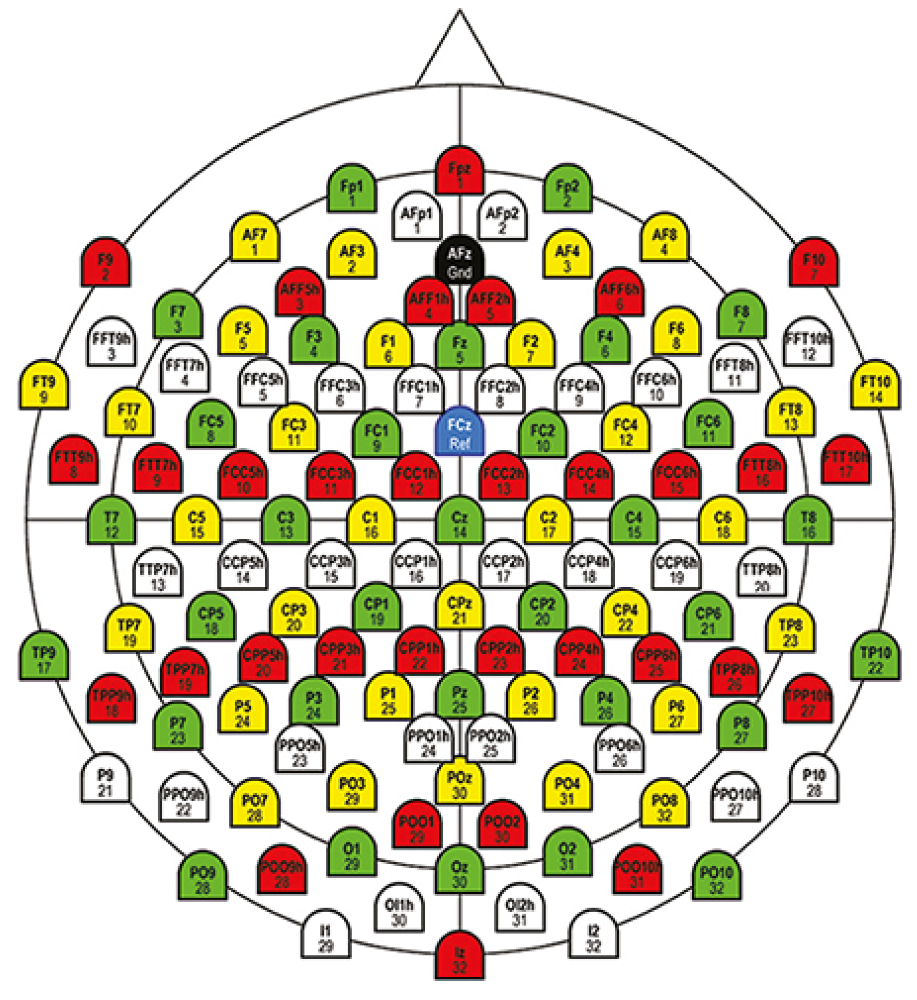
The experiment protocol consisted of instantly visualizing in a continuous sequence, blocks containing images of each label. The display duration of each image block was 0.5 seconds, followed by 10 seconds of recording EEG signals corresponding to the previous visualized block, before considering the same cycle for the adjacent image block. Each image block segment contains EEG signals from 128 channels, recorded with Brainvision DAQs equipment at the sampling frequency of 1 kHz. The data resolution was set to 16 bits. The electrode map of the used system, depicted in Figure 2, is based on the 10–20 placement system. Therefore, Equation 1 presents the number of EEG signal samples corresponding to each channel.

N_{s a m p l e s} = (0.5 s) * 1 k H z = 500

(1)

All channels’ cues were intentionally scratched into 440 samples per task to avoid undesirable signals related to potential interference between the previous and recent image blocks, and also for the uniformization of pattern length purposes. Three band-pass filters were applied to the signals constituting the dataset. That is precisely a second-order Butterworth filter from 5 — 95 Hz, another from 14 — 70 Hz, and the latter one from 55 — 95 Hz, all including a notch filter at 50 Hz. Therefore, 11,964 EEG fragments constitute the current dataset, counting approximately 2,000 segments per subject, since the others were excluded due to mediocre recording quality. Table 2 summarizes the number of signal segments per subject, contained in the referred dataset.

Finally, Table 3 presents the main parameters of the PL dataset released by Spampinato Spampinato et al. [20].

3.3. Mutual Information-Based Channels Selection

The selection of discriminant channels related to the defined mental task aims to gather channels delivering similar information based on entropy values. In the recent literature, similar methods have been proposed to select contributing channels, particularly in [36,40,41]. In this sense, let

M = [1, 2, i, \dots, j, \dots, 128]

be the finite channel set provided by the dataset,

A_{i}

and

B_{j}

two probability distributions of channels i and

j \in M

. The Kullback-Leibler Divergence (KLD) assessing how far a signal joint distribution of i and j channels is from the probability distribution of their products is calculated as,

KLD (A_{i} ∥ B_{j}) = \sum_{a \in M} A_{i} (a) log \frac{A_{i} (a)}{B_{j} (a)},

(2)

where

A_{i} (a)

is the occurrence probability of the

a^{t h}

information. Thus, the MutIn between channel pairs is found by evaluating the KLD as follows:,

\begin{matrix} I (M_{i}; M_{j}) & = K L D (P (M_{i}, M_{j}) ∥ P (M_{i}) P (M_{j})), \end{matrix}

(3)

where

P (M_{i})

and

P (M_{j})

are signal distributions of

M_{i}

and

M_{j}

channels, respectively, and

P (M_{i}, M_{j})

their joint distribution. Generally, calculating MutIn using Equation 3 leads to two cases:

The case where $M_{i}$ and $M_{j}$ are independent, therefore,

$\begin{matrix} I (M_{i}; M_{j}) & = K L D (P (M_{i}, M_{j}) ∥ P (M_{i}) P (M_{j})) = 0 \end{matrix}$

(4)
In other cases, $M_{i}$ and $M_{j}$ channels share the totality of their respective information. Thus,

$\begin{matrix} I (M_{i}; M_{j}) & = K L D (P (M_{i}, M_{j}) ∥ P (M_{i}) P (M_{j})) = H (M_{i}), \end{matrix}$

(5)

where

H (M_{i})

represents the self-entropy of channel

M_{i}

. In this work, making a subset of 64 discriminant channels constitutes a method contribution compared to the state of the art, as will be discussed in Section 4.4. Therefore, when computing Equation 3 according to Algorithm 1, subsets of discriminant channels are constituted by finding maxima cross-entropy values for each considered channel combination.

Algorithm 1:MutIn algorithm-based-discriminant channels selection

The channels selection step typically involves the whole dataset signals. This empirical approach makes a constituted discriminant channel subset more representative of all subjects’ signals. Also, this strategy helps for the cross-subject results comparison purpose. From Algorithm 1, lines 3 to 6 calculate entropies combining two-by-two the 128 channels. Next, a channel combination having a high entropy value is used on lines 10 to 20 to make n-channel combinations by adding one discriminant channel in each iteration until the last 64-channel combination is obtained.

3.4. Enhancing Signals by Minimum-Norm Estimates Algorithm

In the literature related to EEG signal processing, the MNE algorithm and its variants have been used more for brain source localization [42,43], estimation of functional connectivity between different brain cortex [21], and EEG inverse problems [44] than for signals preprocessing [45,46]. Typically, the MNE-Python preprocessing pipeline allows EEG quality assessment provided by selected channels. As a result, EEG segments are extracted using band-stop, band-pass, low-pass, high-pass, and notch filtering [21].

In the present work, semi-automatic functions of MNE-Python were implemented to exclude contaminated EEG data and reduce artifact attenuation. Algorithm 2 summarizes the relevant steps in preprocessing EEG data by MNE.

Algorithm 2:The MNE steps implemented to enhance EEG data.

1 Get EEG data from selected channels

2 Handle poor channels providing extremely noisy data to be usable, based on good signals delivered by other channels.

3 Discard erroneous data gaps and spans.

4 Calculate the variance of the data.

5 Remove the mean and scale to the unit variance to standardize features.

6 Create epoch of data.

7 Average epoch to obtain evoked responses.

The class mne.decoding.Scaler , which includes the steps from 1 to 5 of Algorithm 2 was specifically utilized. This class estimates the mean (

μ

) and variance (

σ

) for each channel by utilizing data from all epochs and time points. That is, the

μ

and

σ

of a given

n^{t h}

training sample are estimated as following:

μ_{n} \approx \frac{1}{N} (\sum_{i = 1}^{N} x_{i}), and

(6)

σ_{n}^{2} \approx \frac{1}{N - 1} \sum_{i = 1}^{N} {(x_{i} - μ_{n})}^{2},

(7)

where N is the number of epochs, and i denotes the time points of each epoch. Therefore, each feature is independently centered and scaled by computing the corresponding statistics on the training set’s samples. By setting

scalings =^{'} {mean}^{'}

, all other parameters of the previously mentioned function were used with their default values, as explained in the implementation documentation [21]. Next, data are fit by standardizing them across channels and then transformed, coupled to their labels to return a new version of epochs data as the output. Hence,

m u

and

σ

are utilized on data by using the MNE’s fit_transform() function. Finally, the obtained epoch is averaged across channels to obtain evoked responses, covering steps 6 to 7 in Algorithm 2.

3.5. The Implemented Classifiers

Two deep learning architecture models are considered, because of their respective performances in processing EEG signals and the outstanding number of referenced works, namely, the EEGNet and a hybrid CNN-LSTM networks [23,47,48].

3.5.1. EEGNet Network

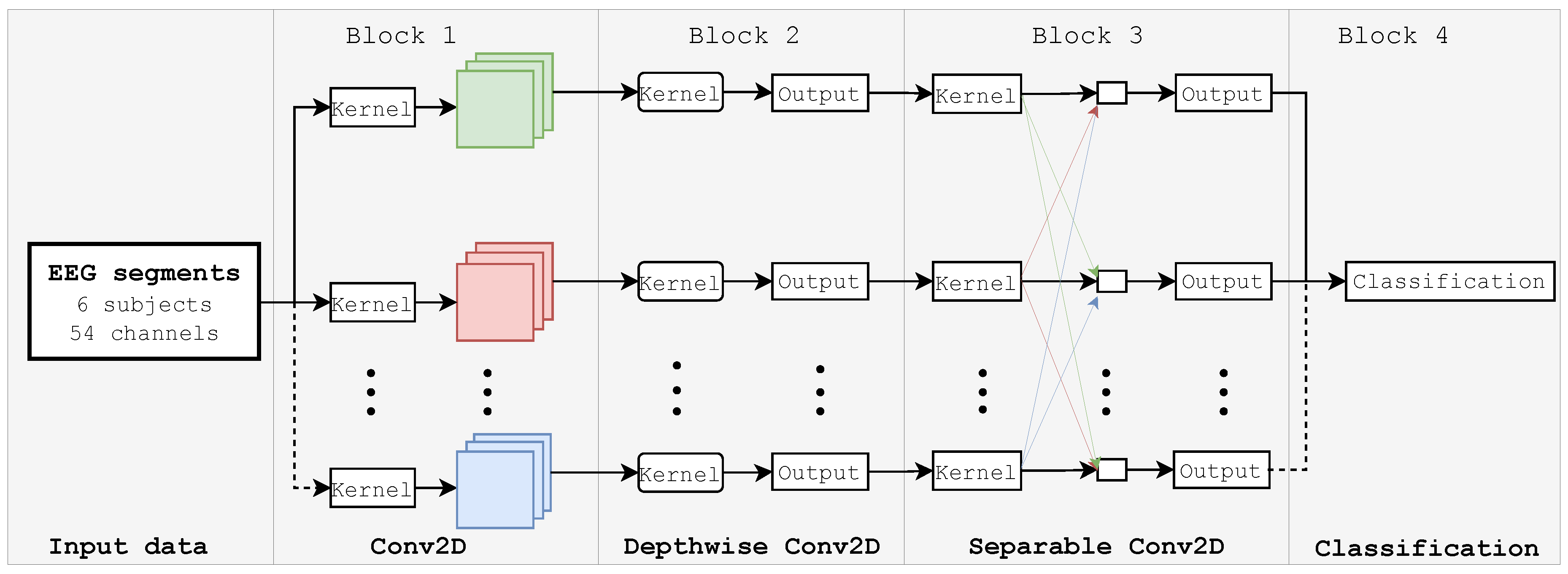
Built in Keras and Tensorflow [49,50], the EEGNet is a compact convolutional neural network proposed by Waytowich et al. [23] for EEG signal processing and classification. The EEGNet architecture takes its use advantage by combining three convolutional layers. That is, a temporal, a depthwise and a separable convolution layer, as illustrated in Figure 3.

Epochs from the MNE block are convolved by the Conv2D (block 1) where frequency filters are applied. After that, each feature map in the Depthwise Conv2D layer (Block 2) is processed by spatial filters to determine its intrinsic properties. Depthwise and pointwise convolutions are executed independently in the Separable Conv2D layer (Block 3) before being combined. Finally, the classification layer (Block 4) evaluates the probability for an output EEG segment to belong to one of the 40 input labels. To do this, the Exponential Linear Unit (ELU) function is used to activate the Depthwise and Separable Conv2D layers, as follows:

f ({\vec{x}}_{i}) = \{\begin{matrix} x_{i} & f o r x \geq 0, \\ α (e^{x_{i}} - 1) & otherwise, \end{matrix}

(8)

and for its part, the dense layer is activated by the Softmax function, given by

σ {(\vec{x})}_{i} = \frac{e^{x_{i}}}{\sum_{j = 1}^{40} e^{x_{j}}}, \forall \vec{x} = {[x_{1}, x_{2}, \dots, x_{40}]}^{⊺},

(9)

where

x_{i}

and

x_{j}

represent the input and output sequences of time points, respectively. The hyper-parameter

α

controlling the saturation point for negative inputs is set to 1. Specifically, the Conv2D layer featured eight temporal filters (F1) with 320 network parameters, the Depthwise Conv2D layer included ten spatial filters (D) with 4320 parameters, and the Separable Conv2D layer possessed 7680 pointwise filters (F2) utilizing 456 parameters. These filters’ values were set up considering the data structure (sampling frequency, length of samples per task and subject, etc.) and the outcomes of preliminary training tests seeking to optimize the classifier. Table 4 summarizes the layers’ main parameters for the proposed EEGNet model.

In addition to this filter setting, the model was built to receive as input 440-time points delivered by the 54 selected channels. Section 4.4 explains the 54-channel selection instead of the 64 targeted. The kernel length was set to 40 to match the number of output classes, with the dropout set to 0.2. Next, the model was compiled using the categorical cross-entropy loss function, the Nadam optimizer, and the accuracy metric, defined in the results section.

3.5.2. The Proposed CNN-LSTM Model

The CNN-LSTM model has proved its efficiency in processing EEG signals for applications-based BCI systems [51,52]. This architecture finds its greatest use in extracting spatial features at the CNN block level. At the same time, temporal dependencies are identified at the LSTM block level, using stronger learning and memory capabilities. Concretely, EEG time points from preprocessing are memorized and forgotten, allowing one to learn more comprehensive features. Because of memory units in the LSTM’s block, the CNN-LSTM model can remember the prior state of the data, ensuring identification based on the current state change pattern. At the end of this hybrid model, a fully connected layer guarantees the labeled output considering an input data sequence. Consequently, Figure 4 presents the proposed CNN-LSTM architecture comprising three CNN layers, two LSTM units, Fully connected, and Softmax layers.

Therefore, the Conv1D_layer1 is configured with 128 convolutions of 3

\times 3

kernel size while Conv1D_layer2 and Conv1D_layer3 layers contain 64 filters of 3

\times 3

size. The He initialization algorithm [53] was used to initialize weights based on a uniform distribution, and the dropout parameter was set to 0.2 for the mentioned layers. All convolutional layers were activated by the leaky Rectified Linear Unit (ReLU) function, given by

f (α, {\vec{x}}_{i}) = \{\begin{matrix} α x_{i} & i f x < 0, \\ x_{i} & otherwise, \forall \vec{x} = {[x_{1}, x_{2}, \dots, x_{40}]}^{⊺} \end{matrix}

(10)

where

α

represent a small positive constant set to 0.005 to compensate negative net inputs with small non-zero gradient. For their part, LSTM layers were configured with 64 and 32 memory units, respectively, to process time point sequences from convolutional layers. At last, the Fully Connected layer contained 54 neurons, and the Softmax layer used 40 neurons to predict the class probability of the output sequence. As in the case of the EEGNet model, the categorical cross-entropy loss function, Nadam optimizer, and accuracy metric were implemented to compile the model. A parameters summary of the proposed CNN-LSTM model is illustrated in Table 5.

3.6. Experimental Settings

The code implementation of both architectures was developed in Python 3.6 using Keras and TensorFlow. An NVIDIA GTX 2080 Ti GPU-equipped Ubuntu 22.04 desktop computer was used to run the entire project. Therefore, to accelerate the learning convergence of the models, the Cyclical Learning Rate (CLR) algorithm [54] was implemented, in addition to helping to avoid local minima in the learning process. The lower and upper bounds of the learning rates were adjusted to

10^{- 3}

and

10^{- 7}

, respectively, by adopting a triangular window, and the step size was set to 8 times the epoch’s total iterations. The EEGNet and CNN-LSTM models were trained at 1000 epochs for comparison purposes, with a batch size set to 440. Finally, the k-fold cross-validation approach presented in Section 4 was used to support the results achieved in this study.

4. Results

The results presented in this section essentially used data presented in Section 3.2, by implementing the k-folds cross-validation method, where k was set to 10. That is, the whole dataset was divided into ten partitions. Consequently, nine partitions were employed iteratively for training, while one partition was used to validate the models’ performance. Specifically, for each of the ten iterations, 10767 samples were used for training and 1197 samples for validation. This validation technique enables the models’ efficiency to be assessed and evaluated for specific data streams or several unpredictable inputs. Additionally, the developed classification approach used the accuracy metric defined by

A c c u r a c y = (\frac{T P + T N}{T P + T N + F P + F N}) \times 100,

(11)

where

T P, T N, F P,

and

F N

represent the true positive, true negative, false positive, and false negative, respectively.

T P

corresponds to each x feature correctly assigned to label X while

T N

represents each x feature of other labels than X unclassified to label X. For its part, opposite to FN, FP is related to all features misclassified to label X. Lastly, the effectiveness of the suggested approach was also assessed using the confusion matrix metric.

4.1. Results Related to Channels Selection

The first step of the developed method consisted of selecting discriminant channels from the 128 provided by the dataset. This study suggests minimizing the number of channels while preserving good classification accuracy since all current deep learning-based studies use all 128 available channels with only a focus on improving classification accuracy. For embedded BCI systems, that have severely constrained computing resources and low power consumption, this accuracy-data size trade-off is essential [55,56]. Therefore, this work proposed using less than half of the available channels by developing Algorithm 1 to select more discriminating channels. Table 6 presents the results achieved in selecting channels.

The developed approach allowed the selection of eight channels in the brain’s parietal cortex and seven in the occipital and parietal-occipital areas. However, only two channels were found to be discriminating in the frontal-central cortex, compared to three in the frontal-central-central area. In sum, EEG signals from the 54 selected channels were considered for the preprocessing step by the MNE method.

4.2. Results of Preprocessing by MNE

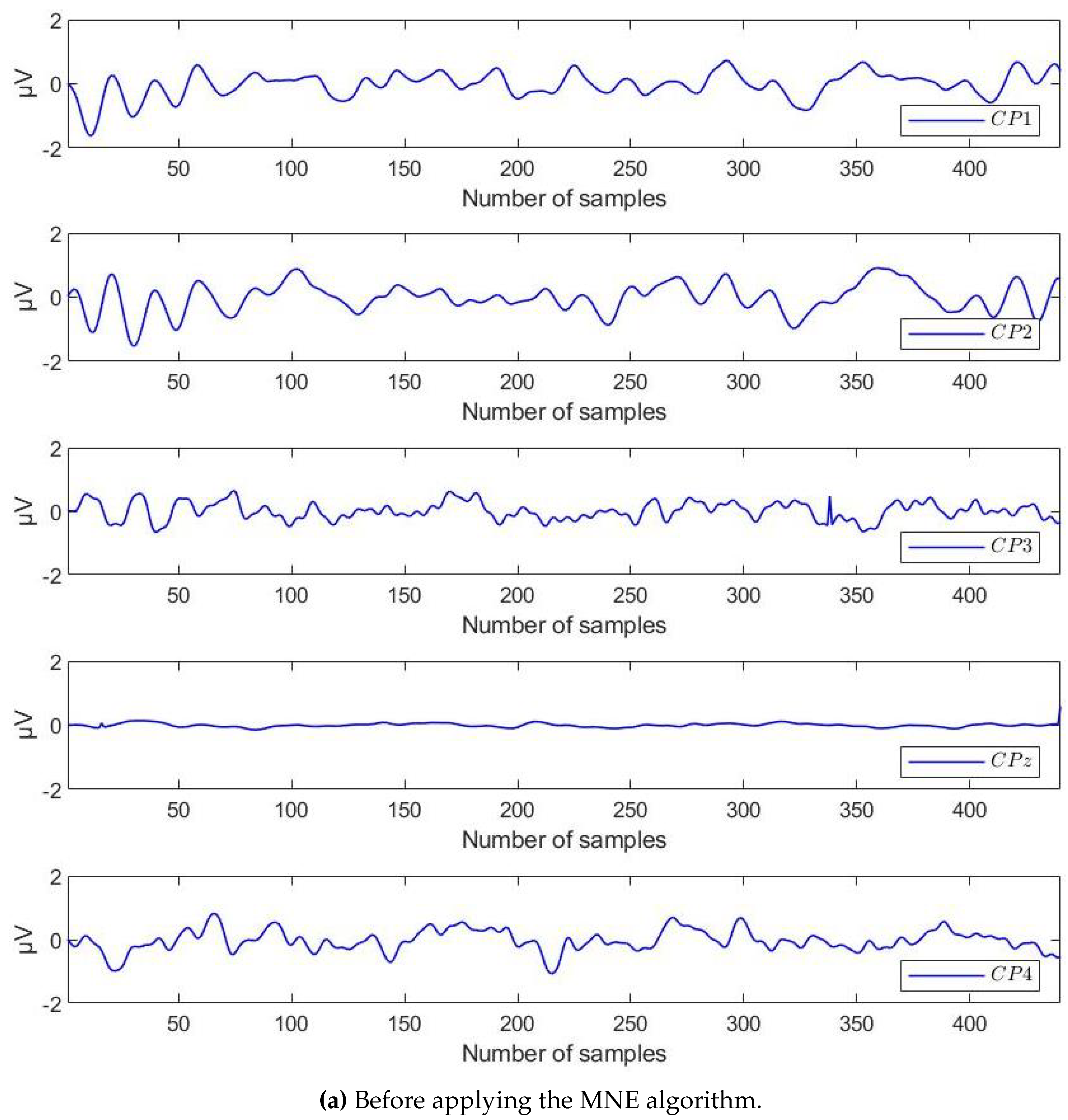
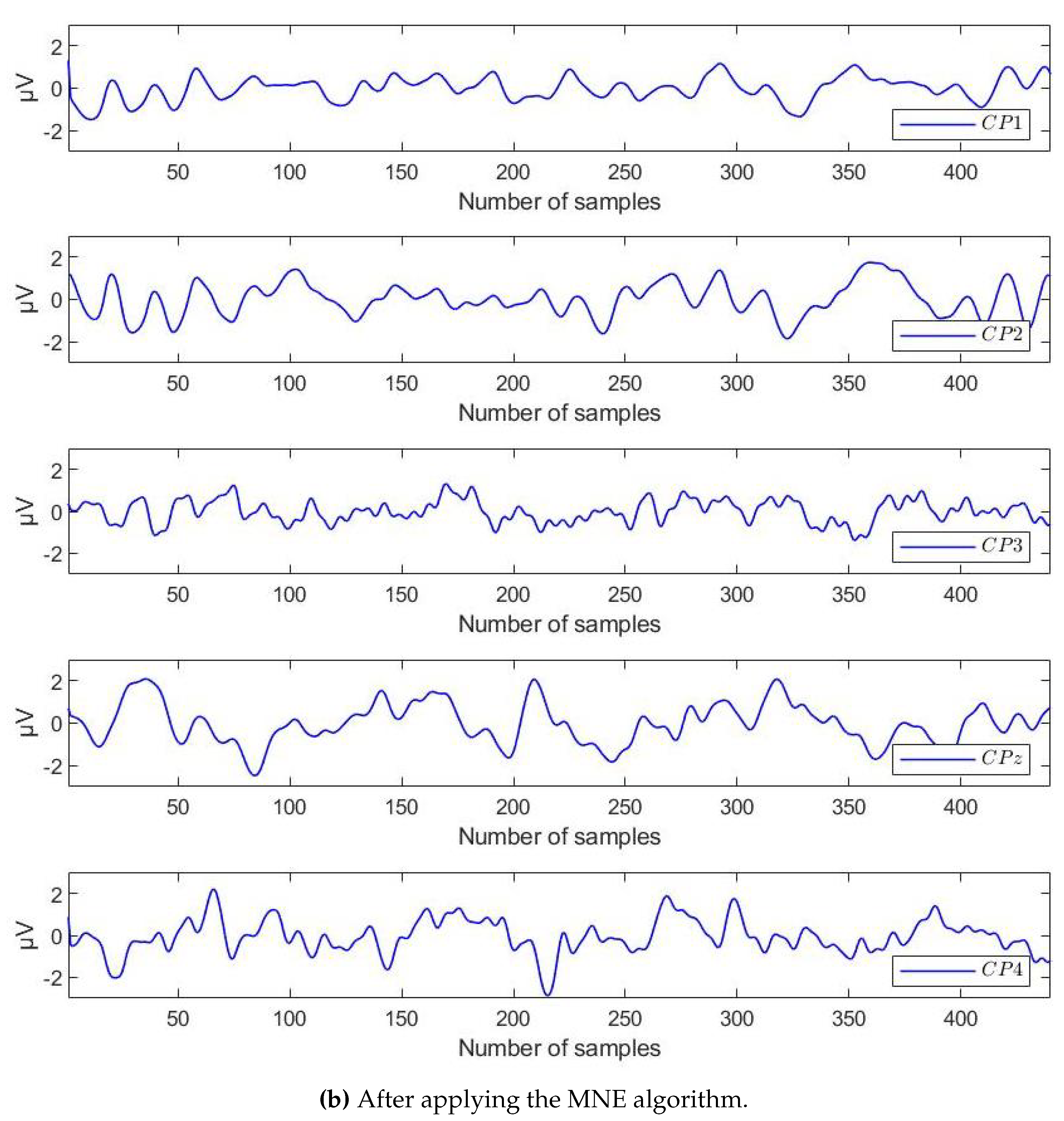
Each EEG segment of the 54 selected channels was enhanced using the MNE algorithm. Therefore, by computing Equations 6 and 7, the length of epochs data was maintained to 440 at the output. As an illustration, Figure 5 presents EEG segments from Subject 4 for a selected group of discriminant channels, before and after implementing the MNE algorithm.

Thus, the new version of epochs data illustrated in Figure 5(b) conserved the class labels of initial data but artifacts were removed through the MNE’s mean scaling procedure. In sum, the data matrix of 11,964 time-point segments from 54 selected channels, containing 440 samples at maximum, was used as input to the classifiers.

4.3. Results Related to EEG Segments Classification

EEG time-point segments were classified according to two approaches. The first one uses a total length of 440 samples. In this sense, Table 7 presents the results achieved by classifying data with the aforementioned models. The classifiers’ accuracy is reported for every

k^{t h}

-fold iteration, alongside the number of segments utilized for testing and training. The average accuracy of 93.2 and 88.2% were reached in classifying data into 40 labels, by using the EEGNet and CNN-LSTM networks, respectively.

The second approach considers different sample lengths to evaluate the signal stretches with data more enhanced by the preprocessing step.

Therefore, Table 8 considers nine data time intervals between 20 and 440 samples. This stretch cutting was motivated by the following considerations. On the one hand, looking to evaluate the length of 440 samples in small stretches, leaving out data samples at one extremity. On the other hand, to compare the outcomes of the suggested method with those of the state-of-the-art (SOTA), the selected stretch lengths were assumed. Thus, the classification accuracies reported in Table 8 are averaged from those achieved by each k-fold iteration. The best average accuracy of 94.8% was reached by processing data in 360 - 440 ms, while the lowest of 87.2% was obtained for data in 20 - 240 ms with the EEGNet model. For its part, the CNN-LSTM architecture best performed the classification task by processing the 360-440 ms stretch (89.8%) rather than for the 20-240 ms one (81.3%). In summary, the developed strategy of samples’ stretch-splitting enabled different outcomes, a pertinent observation discussed in the next section. Furthermore, Table 9 and Table 10 present the summary results of the confusion matrices classifying data segments according to each class label. The diagonal results of the confusion matrix, displayed in the tables afterward, illustrate the exactness of predicted versus true labels for a specific output class.

Therefore, the CNN-LSTM model outperformed the data class labeling in the 240-440 ms stretch, followed by the 360-440 ms, 130-350 ms, and 130-440 ms stretches, by achieving accuracies of 93, 92, 91, and 90%, respectively. On another side, accuracies of 88, 87, and 86% were obtained by processing stretches of 360-440 ms, 130-440, 130-350 ms, and 240-440 ms, in this order, with the CNN-LSTM classifier.

4.4. Discussion

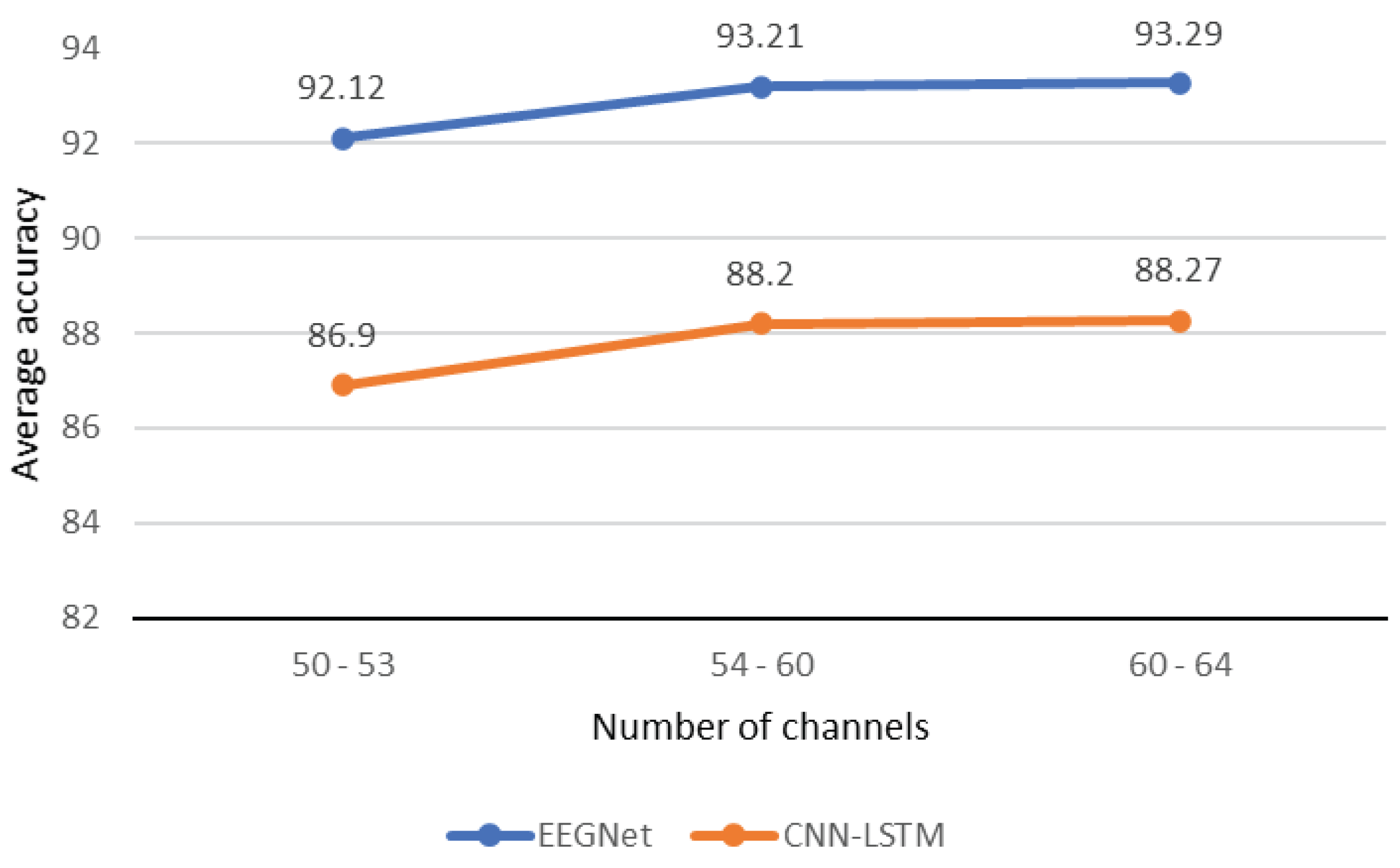
One of this work’s important contributions is optimizing the number of contributing channels while ensuring accurate data classification for BCI applications. A subsequent check of discriminant frames was introduced to deduce signal lengths more enhanced by the MNE preprocessing. Regarding the number of channels, this work aimed to use less than 50% of the available channels. This is to deal, on the one hand, with one of the current big data processing issues for embedded BCI applications, where computational resources are constrained, for instance [57]. On the other hand, selecting discriminating channels allowed to minimize the influence of channels whose intrinsic characteristics do not contribute significantly to the classification process, based on the information conveyed [58]. Thus, Algorithm 1 was configured to select 64 channels from the 128 available, based essentially on the mutual information evaluated using the cross-entropies. After configuring the classifiers, the first tests aimed to set Algorithm 1 for a limit of 60 channels, assess the outcomes, and then compare them with those achieved with 64 channels. The differences between outcomes were minimal compared to the large amount of data to be conserved in the processing chain by considering the 64 channels. Comparing the outcomes of 55 channels with those of 60 and 64 channels resulted in the same finding. However, by proceeding with the same approach between 50 and 55 channels, it was uncovered that 53 of the ones selected provided a larger difference than 54 channels, as illustrated in Figure 6.

Consequently, for the remaining processing steps, the concluding selection of 54 channels was determined. Therefore, from the 54 channels selected, 33 are located in the parietal-occipital cortex and 16 in the central cortex. In other words, the mental task of image visualization produced a greater neuronal effect on the motor and visual cortices than in others, as reported by Zheng and Chen [30].

Next, preprocessing by MNE allowed for obtaining the data enhanced, and more suitable for the classifiers. Table 11 presents the obtained results with and without MNE’s preprocessing block integration.

In the case of the EEGNet network, an average relative benefit of 12.8% was evaluated by implementing the MNE’s preprocessing stage, whereas the CNN-LSTM classifier for its part, enabled achieving a relative gain of 13.9%.

The final step of data classification was carried out by the EEGNet and CNN-LSTM models. The better performance of the EEGNet architecture compared to the CNN-LSTM model was observed, based on the metrics presented above. Essentially built around distinct architectures, the CNN-LSTM model required roughly 107278 parameters whilst only 54632 parameters were used to configure the EEGNet network, almost half the number of parameters utilized by the CNN-LSTM model. This finding gives credence, in addition to the performance achieved, to the EEGNet network for embedded BCI applications, for the above-mentioned reasons.

When comparing the outcomes obtained in this work with those reported in related literature, essentially based on handling the PL dataset, the overview observation is that all use data provided by the 128 channels, as summarized in Table 12. In contrast, in this work, the number of channels was reduced by about 57.8% compared to that used by the references. This is one of the key contributions of the proposed method, placing this last one explicitly in the field of embedded BCI systems.

In the last column of Table 12, classification accuracies are compared. Spampinato [20] and Nandini [32] obtained accuracies of 82.9 and 81.59% by implementing RNN/CNN and STFT+EEGCapsNet models, respectively. The proposed approach with both architectures better performed the class labeling task than the evoked works. On the other side, Xiao [30,31] and Nastaran Khaleghi et al. [33] reported accuracies of 99.50, 97.13, and 98.4% by using Bi-LSTM-AttGW, LSTMs_B, and FC-GDN architectures. Their achievement exceeds the outcomes obtained in this framework by an average of 3.5%. However, the accuracy discrepancy compared to the benefit recorded utilizing fewer than half of the available channels is thereby acceptable, considering further that the recommended accuracy for BCI applications is valued above 70%. In other words, processing data provided by the whole set of channels to improve the average accuracy only of 3.5% seems to expend computational resources excessively than optimizing the number of useful channels. Therefore, this work proposes a reliable alternative for embedded BCI applications, offering a suitable trade-off accuracy-computational time.

5. Conclusion

This section is presented in two steps. In the first one, the conclusion of this work is provided by summarizing the interpretation of the results obtained and the developed method scope. In the second part, upcoming work is contemplated based on the results achieved, considering this achievement as the initial phase of an ambitious project to be developed.

5.1. Conclusion

This work aimed to classify EEG visualization signals into 40 labels, that is, dealing with the recent EEG visual multiclass classification challenge, by using a smaller number of channels while maintaining reliable classification accuracy. Public data from the PL dataset including 11964 EEG signal segments were used for the experiment. To be more specific, a set of 54 discriminating channels was built using a channel selection approach based on mutual information. Next, data were enhanced using the MNE method. In the last stage, the EEGNet and CNN-LSTM architectures served as classifiers to label data according to the defined classes. The results achieved demonstrate a good performance of the EEGNet classifier over the CNN-LSTM, by reaching the highest accuracy of 94.8%. Compared with the models proposed in the related literature, this work incorporates the trade-off between the classification accuracy and the number of channels. The latest is a more desired criterion in the implementation of embedded BCI systems based on EEG signals. However, the results presented in this work are constrained to the configuration set in the preprocessing and classification blocks. Also on the use of data provided by the PL database, exclusively. The source codes of this project are available to the public at https://github.com/Tatyvelu/EEG-Visual-Multiclass-Classification.

5.2. Forthcoming Work

The challenge of database availability with more than 40 classes, similar to the PL dataset, motivates forward a multiclass database construction, consisting of EEG signals from fruit sequences visualization. Such a dataset would be useful for implementing the EEGNet model in the NAO robot to assist people in fruit type recognition.

Author Contributions

Conceptualization, T.M.-V.; data curation, T.M.-V., J.R.-P.; formal analysis, J.R.-P.; funding acquisition, E.Z.-G. and J.H.S.-A.; investigation, T.M.-V., J.R.-P., E.Z.-G., J.I.V.-G., and J.H.S-A.; methodology, T.M.-V. and E.Z.-G.; software, T.M.-V. and J.R.-P.; validation, J.R.-P. and E.Z.-G.; writing–original draft, T.M.-V.; writing–review and editing, T.M.-V., E.Z.-G, J.R.-P. and J.I.V.-G. All authors read and agreed to the published version of the manuscript.

Funding

This work was supported by the Centro de Investigación en Computación - Insituto Politécnico Nacional through the Dirección de Investigación (Folio SIP/1988/DI/DAI/2022, 20220002, 20230232, 20240108, 20231622, 20240956), and the Mexican National Council of Humanity, Science and Technology CONAHCyT under the postdoctoral grant 2022-2024 CVU No. 763527.

Institutional Review Board Statement

Ethical review and approval are waived for this study.

Informed Consent Statement

No Formal written consent was required for this study.

Data Availability Statement

Data available under a formal demand.

Conflicts of Interest

The authors declare no conflict of interest. The funders had no role in the design of this study; in the collection, analyses, or data interpretation; in the manuscript writing, or in the decision to publish the results.

Abbreviations

BCI	Brain-Computer Interface
EEG	Electroencephalogram
CSP	Common Spatial Pattern
SVM	Support Vector Machine
DCNN	Deep Convolutional Neural Network
LSTM	Long-Short-Term Memory
fNIRS	Functional near-infrared spectroscopy
SD	Source-detector
RNN	Recurrent Neural Network
CNN	Convolutional Neural Network
EEGNet	Compact convolutional neural network for EEG-based BCI
PL	Perceive Lab
CNN-LSTM	Convolutional Neural Network-Long-Short Term Memory
ERP	Event-related potential
STFT	Short-Term Fourier Transform
VEP	Visual-evoked potentials
SSVEP	Steady-State Visually Evoked Potentials
KNN	K-nearest neighbors
EEGCapsNet	Capsule Network
FC-GDN	Functional connectivity-based geometric deep network
MutIn	Mutual Information
MNE	Minimum-Norm Estimates software suite
MI	Motor Imagery
MI-EEG	Motor Imagery EEG
EVC	EEG Visual Classification
EMG	Electromyogram
KLD	Kullback-Leibler Divergence
CLR	Cyclical Learning Rate
SOTA	State-of-the-art

References

Abdulwahab, S.S.; Khleaf, H.K.; Jassim, M.H.; Abdulwahab, S. A Systematic Review of Brain-Computer Interface Based EEG. Iraqi J. Electr. Electron. Eng 2020, 16, 1–10. [Google Scholar] [CrossRef]
Pereira, C.D.; Martins, F.; Marques, F.; Sousa, J.C.; Rebelo, S. Beyond Brain Signaling. Tissue-Specific Cell Signaling 2020, 1–32. [Google Scholar]
Sharma, P.C.; Raja, R.; Vishwakarma, S.K.; Sharma, S.; Mishra, P.K.; Kushwah, V.S. Analysis of brain signal processing and real-time EEG signal enhancement. Multimedia Tools and Applications 2022, 81, 41013–41033. [Google Scholar] [CrossRef]
Zhang, Z.; Han, S.; Yi, H.; Duan, F.; Kang, F.; Sun, Z.; Solé-Casals, J.; Caiafa, C.F. A brain-controlled vehicle system based on steady state visual evoked potentials. Cognitive Computation 2023, 15, 159–175. [Google Scholar] [CrossRef]
Belkacem, A.N.; Lakas, A. A cooperative EEG-based BCI control system for robot–drone interaction. 2021 International Wireless Communications and Mobile Computing (IWCMC). IEEE, 2021, pp. 297–302.
Choi, J.; Kim, K.T.; Jeong, J.H.; Kim, L.; Lee, S.J.; Kim, H. Developing a motor imagery-based real-time asynchronous hybrid BCI controller for a lower-limb exoskeleton. Sensors 2020, 20, 7309. [Google Scholar] [CrossRef]
Belwafi, K.; Ghaffari, F.; Djemal, R.; Romain, O. A hardware/software prototype of EEG-based BCI system for home device control. Journal of Signal Processing Systems 2017, 89, 263–279. [Google Scholar] [CrossRef]
Feng, Z.; Sun, Y.; Qian, L.; Qi, Y.; Wang, Y.; Guan, C.; Sun, Y. Design a novel BCI for neurorehabilitation using concurrent LFP and EEG features: A case study. IEEE Transactions on Biomedical Engineering 2021, 69, 1554–1563. [Google Scholar] [CrossRef]
Nandikolla, V.; Medina Portilla, D.A.; others. Teleoperation robot control of a hybrid eeg-based bci arm manipulator using ros. Journal of Robotics 2022, 2022. [Google Scholar] [CrossRef]
Tariq, M.; Trivailo, P.M.; Simic, M. EEG-based BCI control schemes for lower-limb assistive-robots. Frontiers in human neuroscience 2018, 12, 312. [Google Scholar] [CrossRef]
Kobayashi, N.; Nakagawa, M. BCI-based control of electric wheelchair using fractal characteristics of EEG. IEEJ Transactions on Electrical and Electronic Engineering 2018, 13, 1795–1803. [Google Scholar] [CrossRef]
Onose, G.; Grozea, C.; Anghelescu, A.; Daia, C.; Sinescu, C.J.; Ciurea, A.V.; Spircu, T.; Mirea, A.; Andone, I.; Spânu, A.; others. On the feasibility of using motor imagery EEG-based brain–computer interface in chronic tetraplegics for assistive robotic arm control: a clinical test and long-term post-trial follow-up. Spinal cord 2012, 50, 599–608. [Google Scholar] [CrossRef] [PubMed]
Zhu, Y.; Li, Y.; Lu, J.; Li, P. A hybrid BCI based on SSVEP and EOG for robotic arm control. Frontiers in neurorobotics 2020, 14, 583641. [Google Scholar] [CrossRef] [PubMed]
Del Moral, P.; Nowaczyk, S.; Pashami, S. Why is multiclass classification hard? IEEE Access 2022, 10, 80448–80462. [Google Scholar] [CrossRef]
Kurgansky, A. Functional organization of the human brain in the resting state. Neuroscience and Behavioral Physiology 2019, 49, 1135–1144. [Google Scholar] [CrossRef]
Das, S.; Tripathy, D.; Raheja, J.L. Real-time BCI system design to control arduino based speed controllable robot using EEG; Springer, 2019.
Mahmood, A.; Zainab, R.; Ahmad, R.B.; Saeed, M.; Kamboh, A.M. Classification of multi-class motor imagery EEG using four band common spatial pattern. 2017 39th Annual International Conference of the IEEE Engineering in Medicine and Biology Society (EMBC). IEEE, 2017, pp. 1034–1037.
Fadel, W.; Kollod, C.; Wahdow, M.; Ibrahim, Y.; Ulbert, I. Multi-class classification of motor imagery EEG signals using image-based deep recurrent convolutional neural network. 2020 8th International Winter Conference on Brain-Computer Interface (BCI). IEEE, 2020, pp. 1–4.
Kwon, J.; Shin, J.; Im, C.H. Toward a compact hybrid brain-computer interface (BCI): Performance evaluation of multi-class hybrid EEG-fNIRS BCIs with limited number of channels. PloS one 2020, 15, e0230491. [Google Scholar] [CrossRef] [PubMed]
Spampinato, C.; Palazzo, S.; Kavasidis, I.; Giordano, D.; Souly, N.; Shah, M. Deep learning human mind for automated visual classification. Proceedings of the IEEE conference on computer vision and pattern recognition, 2017, pp. 6809–6817.
Gramfort, A.; Luessi, M.; Larson, E.; Engemann, D.; Strohmeier, D.; Brodbeck, C.; Goj, R.; Jas, M.; Brooks, T.; Parkkonen, L. ; others. MEG and EEG data analysis with MNE-Python. frontiers in Neuroscience, 267, 2013.
Esch, L.; Dinh, C.; Larson, E.; Engemann, D.; Jas, M.; Khan, S.; Gramfort, A.; Hämäläinen, M.S. MNE: software for acquiring, processing, and visualizing MEG/EEG data. Magnetoencephalography: From Signals to Dynamic Cortical Networks 2019, 355–371. [Google Scholar]
Waytowich, N.; Lawhern, V.J.; Garcia, J.O.; Cummings, J.; Faller, J.; Sajda, P.; Vettel, J.M. Compact convolutional neural networks for classification of asynchronous steady-state visual evoked potentials. Journal of neural engineering 2018, 15, 066031. [Google Scholar] [CrossRef] [PubMed]
Shoji, T.; Yoshida, N.; Tanaka, T. Automated detection of abnormalities from an EEG recording of epilepsy patients with a compact convolutional neural network. Biomedical Signal Processing and Control 2021, 70, 103013. [Google Scholar] [CrossRef]
Rashid, M.; Sulaiman, N.; PP Abdul Majeed, A.; Musa, R.M.; Ab Nasir, A.F.; Bari, B.S.; Khatun, S. Current status, challenges, and possible solutions of EEG-based brain-computer interface: a comprehensive review. Frontiers in neurorobotics 2020, 14, 515104. [Google Scholar] [CrossRef]
Nakagome, S.; Craik, A.; Sujatha Ravindran, A.; He, Y.; Cruz-Garza, J.G.; Contreras-Vidal, J.L. Deep learning methods for EEG neural classification. In Handbook of Neuroengineering; Springer, 2022; pp. 1–39.
Yedukondalu, J.; Sharma, L.D. Cognitive load detection using circulant singular spectrum analysis and Binary Harris Hawks Optimization based feature selection. Biomedical Signal Processing and Control 2023, 79, 104006. [Google Scholar] [CrossRef]
Kanaga, E.G.M.; Thanka, M.R.; Anitha, J. ; others. A Pilot Investigation on the Performance of Auditory Stimuli based on EEG Signals Classification for BCI Applications. 2022 Third International Conference on Intelligent Computing Instrumentation and Control Technologies (ICICICT). IEEE, 2022, pp. 632–637.
Kalafatovich, J.; Lee, M.; Lee, S.W. Learning Spatiotemporal Graph Representations for Visual Perception Using EEG Signals. IEEE Transactions on Neural Systems and Rehabilitation Engineering 2022, 31, 97–108. [Google Scholar] [CrossRef]
Zheng, X.; Chen, W. An attention-based bi-LSTM method for visual object classification via EEG. Biomedical Signal Processing and Control 2021, 63, 102174. [Google Scholar] [CrossRef]
Zheng, X.; Chen, W.; You, Y.; Jiang, Y.; Li, M.; Zhang, T. Ensemble deep learning for automated visual classification using EEG signals. Pattern Recognition 2020, 102, 107147. [Google Scholar] [CrossRef]
Kumari, N.; Anwar, S.; Bhattacharjee, V. Automated visual stimuli evoked multi-channel EEG signal classification using EEGCapsNet. Pattern Recognition Letters 2022, 153, 29–35. [Google Scholar] [CrossRef]
Khaleghi, N.; Rezaii, T.Y.; Beheshti, S.; Meshgini, S. Developing an efficient functional connectivity-based geometric deep network for automatic EEG-based visual decoding. Biomedical Signal Processing and Control 2023, 80, 104221. [Google Scholar] [CrossRef]
Seeck, M.; Koessler, L.; Bast, T.; Leijten, F.; Michel, C.; Baumgartner, C.; He, B.; Beniczky, S. The standardized EEG electrode array of the IFCN. Clinical neurophysiology 2017, 128, 2070–2077. [Google Scholar] [CrossRef]
Daud, S.S.; Sudirman, R. Decomposition level comparison of stationary wavelet transform filter for visual task electroencephalogram. Jurnal Teknologi 2015, 74. [Google Scholar]
Baig, M.Z.; Aslam, N.; Shum, H.P. Filtering techniques for channel selection in motor imagery EEG applications: a survey. Artificial intelligence review 2020, 53, 1207–1232. [Google Scholar] [CrossRef]
Das, A.; Suresh, S. An effect-size based channel selection algorithm for mental task classification in brain computer interface. 2015 IEEE International Conference on Systems, Man, and Cybernetics. IEEE, 2015, pp. 3140–3145.
Deng, J.; Dong, W.; Socher, R.; Li, L.J.; Li, K.; Fei-Fei, L. Imagenet: A large-scale hierarchical image database. 2009 IEEE conference on computer vision and pattern recognition. Ieee, 2009, pp. 248–255.
Palazzo, S.; Spampinato, C.; Kavasidis, I.; Giordano, D.; Schmidt, J.; Shah, M. Decoding brain representations by multimodal learning of neural activity and visual features. IEEE Transactions on Pattern Analysis and Machine Intelligence 2020, 43, 3833–3849. [Google Scholar] [CrossRef]
Wang, Z.M.; Hu, S.Y.; Song, H. Channel selection method for EEG emotion recognition using normalized mutual information. IEEE Access 2019, 7, 143303–143311. [Google Scholar] [CrossRef]
De Clercq, P.; Vanthornhout, J.; Vandermosten, M.; Francart, T. Beyond linear neural envelope tracking: a mutual information approach. Journal of Neural Engineering 2023, 20, 026007. [Google Scholar] [CrossRef] [PubMed]
Li, M.a.; Wang, Y.f.; Sun, Y.j. Minimum norm estimates based dipole source estimation. BIBE 2018; International Conference on Biological Information and Biomedical Engineering. VDE, 2018, pp. 1–5.
Jatoi, M.A.; Kamel, N. Brain source localization using reduced EEG sensors. Signal, Image and video processing 2018, 12, 1447–1454. [Google Scholar] [CrossRef]
Jatoi, M.A.; Kamel, N.; Teevino, S.H. Trend analysis for brain source localization techniques using EEG signals. 2020 3rd International Conference on Computing, Mathematics and Engineering Technologies (iCoMET). IEEE, 2020, pp. 1–5.
Kyriaki, K.; Koukopoulos, D.; Fidas, C.A. A Comprehensive Survey of EEG Preprocessing Methods for Cognitive Load Assessment. IEEE Access 2024. [Google Scholar] [CrossRef]
Hauk, O. Keep it simple: a case for using classical minimum norm estimation in the analysis of EEG and MEG data. Neuroimage 2004, 21, 1612–1621. [Google Scholar] [CrossRef] [PubMed]
Li, K.; Ao, B.; Wu, X.; Wen, Q.; Ul Haq, E.; Yin, J. Parkinson’s disease detection and classification using EEG based on deep CNN-LSTM model. Biotechnology and Genetic Engineering Reviews 2023, 1–20. [Google Scholar] [CrossRef] [PubMed]
Efe, E.; Ozsen, S. CoSleepNet: Automated sleep staging using a hybrid CNN-LSTM network on imbalanced EEG-EOG datasets. Biomedical Signal Processing and Control 2023, 80, 104299. [Google Scholar] [CrossRef]
Chollet, F. others 2015; Keras. GitHub. Retrieved fromhttps. github. com/fchollet/keras.
Abadi, M.; Agarwal, A.; Barham, P.; Brevdo, E.; Chen, Z.; Citro, C.; Corrado, G.S.; Davis, A.; Dean, J.; Devin, M. ; others. TensorFlow: Large-scale machine learning on heterogeneous systems, 2015.
Wang, X.; Wang, Y.; Liu, D.; Wang, Y.; Wang, Z. Automated recognition of epilepsy from EEG signals using a combining space–time algorithm of CNN-LSTM. Scientific Reports 2023, 13, 14876. [Google Scholar] [CrossRef]
Shoeibi, A.; Rezaei, M.; Ghassemi, N.; Namadchian, Z.; Zare, A.; Gorriz, J.M. Automatic diagnosis of schizophrenia in EEG signals using functional connectivity features and CNN-LSTM model. International work-conference on the interplay between natural and artificial computation. Springer, 2022, pp. 63–73.
Yam, J.Y.; Chow, T.W. A weight initialization method for improving training speed in feedforward neural network. Neurocomputing 2000, 30, 219–232. [Google Scholar] [CrossRef]
Smith, L.N. Cyclical learning rates for training neural networks. 2017 IEEE winter conference on applications of computer vision (WACV). IEEE, 2017, pp. 464–472.
Wang, X.; Hersche, M.; Magno, M.; Benini, L. Mi-bminet: An efficient convolutional neural network for motor imagery brain–machine interfaces with eeg channel selection. IEEE Sensors Journal 2024. [Google Scholar] [CrossRef]
Belwafi, K.; Romain, O.; Gannouni, S.; Ghaffari, F.; Djemal, R.; Ouni, B. An embedded implementation based on adaptive filter bank for brain–computer interface systems. Journal of neuroscience methods 2018, 305, 1–16. [Google Scholar] [CrossRef]
Kumar, Y.; Kumar, J.; Sheoran, P. Integration of cloud computing in BCI: A review. Biomedical Signal Processing and Control 2024, 87, 105548. [Google Scholar] [CrossRef]
Mwata-Velu, T.; Avina-Cervantes, J.G.; Ruiz-Pinales, J.; Garcia-Calva, T.A.; González-Barbosa, E.A.; Hurtado- Ramos, J.B.; González-Barbosa, J.J. Improving motor imagery eeg classification based on channel selection using a deep learning architecture. Mathematics 2022, 10, 2302. [Google Scholar] [CrossRef]

Figure 1. High-level general diagram of the proposed method. EEG visualization signals from 128 channels are provided by the public dataset published in [20]. Next, 64 channels are selected from the 128 provided by evaluating the channels’ MutIn. Therefore, the MNE algorithm is applied to enhance EEG data which are classified into 40 labels, by the EEGNet and CNN-LSTM architectures, separately.

Figure 2. The EEG actiCAP 128-channels standard layout used for the experiment protocol, modified from [39]. A total of 128 electrodes are illustrated in four colors (green, yellow, red, and white in this order), i.e., 32 active electrodes for each color group. Capital letters in electrode taxonomy typically indicate the spatial location over the brain cortex: T for temporal, Fp for frontal, C for central, P for parietal, and O for the occipital cortex. A classic combination of two letters means that the electrode is placed over the intermediate area between two brain cortices.

Figure 3. The EEGNet architecture. Conv2D extracts temporal features in the first block. Feature maps are enhanced in Block 2 using spatial filters and combined in Separable Conv2D. Finally, Block 4 estimates the output probability for a processed feature map.

Figure 4. The implemented CNN-LSTM architecture. Two 1D-CNN layers separated by a Max-Pooling layer represent the input block of the model. Next, a cascade of LSTM-1DCNN-LSTM performs the feature learning and extraction. At last, the label output probability is computed by the Softmax layer, which is coupled to the Fully Connected layer.

Figure 5. EEG segments of Subject 4 before (a) and after (b) application of the MNE algorithm to data from channels

C P 1, C P 2, C P 3, C P z,

and

C P 4

. The maximum length of segments is 440.

Figure 5. EEG segments of Subject 4 before (a) and after (b) application of the MNE algorithm to data from channels

C P 1, C P 2, C P 3, C P z,

and

C P 4

. The maximum length of segments is 440.

Figure 6. Illustration of the number of channels setting. As shown in the figure, the observable change in classification accuracy occurs by reducing the number of channels beyond 54, after selecting the targeted 64.

Table 1. The PL dataset in the recent literature.

Works	Models	Dataset	Channels	Acc. [%]
Zheng and Chen [30]	Bi-LSTM-AttGW	PL	128	99.50
Zheng et al. [31]	LSTMS_B	PL	128	97.13
Spampinato et al. [20]	RNN/CNN	PL	128	82.9
Kumari et al. [32]	STFT + EEGCapsNet	PL	128	81.59
Khaleghi et al. [33]	FC-GDN	PL	128	98.4

Table 2. The number of samples by subject in the EEG visual dataset.

Order	Subject	Segments order	Number of samples
1	4	from 1 to 1995	1995
2	1	from 1996 to 3980	1985
3	6	from 3981 to 5976	1996
4	3	from 5977 to 7972	1996
5	2	from 7973 to 9968	1996
6	5	from 9969 to 11964	1996
Total	All subjects	from 1 to 11964	11964

Table 3. The summary of the experiment protocol parameters.

Parameter	Number
Total number of images	2000
Number of images per class	50
Number of classes	40
Display mode	sequential
Display time per image	0.5 s
Sampling frequency	1000 Hz
Pause time between classes	10 s
Number of sessions	4
Session running time	350 s
Total running time	1400 s

Table 4. Main layers’ parameters for the proposed EEGNet model.

Layer (type)	Output Shape	Parameters
Input Layer	(None, 54, 440, 1)	0
Conv2D	(None, 54, 440, 8)	320
Batch_normalization_1	(None, 54, 440, 8)	32
Depthwise_conv2D	(None, 1, 440, 80)	4320
Batch_normalization_2	(None, 1, 440, 80)	320
Activation_1	(None, 1, 440, 80)	0
Average_pooling2D_1	(None, 1, 110, 80)	0
Dropout_1	(None, 1, 110, 80)	0
Separable_conv2D	(None, 1, 110, 80)	7680
Batch_normalization_3	(None, 1, 110, 80)	320
Activation_2	(None, 1, 110, 80)	0
Average_pooling2D_2	(None, 1, 13, 80)	0
Dropout_2	(None, 1, 13, 80)	0
Flatten	(None, 1040)	0
Dense	(None, 40)	41640
Softmax	(None, 40)	0

Table 5. Parameters summary of the proposed CNN-LSTM model

Layer (type)	Output Shape	Parameters
Conv1D_layer1	(None, 440, 128)	20864
Dropout_1	(None, 440, 128)	0
Activation_1	(None, 440, 128)	0
Max_Pooling	(None, 220, 128)	0
Conv1D_layer2	(None, 220, 64)	24640
Dropout_2	(None, 220, 64)	0
Activation_2	(None, 220, 64)	0
LSTM_layer1	(None, 220, 64)	33024
Conv1D_layer3	(None, 220, 64)	12352
Dropout_3	(None, 220, 64)	0
Activation_3	(None, 220, 64)	0
LSTM_layer2	(None, 32)	12416
Dropout_4	(None, 32)	0
Dense_1	(None, 54)	1782
Activation_4	(None, 54)	0
Dense_2	(None, 40)	2200

Table 6. Channels selected applying Algorithm 1. The term Nr.Ch. in the second column refers to the number of channels.

Brain Area	Nr.Ch.	Description
Frontal-Central-Central	3	FCC1h,FCC2h,FCC4h
Frontal-Central	2	FC1,FC2,
Central	7	C1,C2,C3,Cz,C4,C5,C6
Central-Parietal	5	CP1,CP2,CP3,CPz,CP4
Central-Central-Parietal	4	CCP1h,CCP2h,CCP3h,CCP4h
Occipital	7	O1,Oz,O2,I1,O11h,O12h,I2
Parietal	8	Pz,P1,P2,P3,P4,P5,P6,P8
Parietal-Occipital	7	PO7,PO3,POz,PO4,PO8,PO9,PO10
Parietal-Parietal-Occipital	6	PPO9h,PPO5h,PPO1h,PPO2h,PPO6h, PPO10h
Parietal-Occipital-Occipital	5	POO1,POO2,POO9h,POO10h,Iz
TOTAL	54

Table 7. Achieved accuracy in each k-fold iteration by the two proposed classifiers, setting the time interval to 440 samples.

k-fold	Number of segments		Classification accuracy [%]
	Training	Testing	EEGNet	CNN-LSTM
1	10768	1197	92.8	88.7
2	10768	1197	93.1	88.9
3	10768	1197	92.2	89.1
4	10768	1197	93.6	87.3
5	10768	1197	94.3	88.8
6	10769	1196	93.7	88.2
7	10769	1196	92.8	87.9
8	10769	1196	94.1	88.1
9	10769	1196	92.9	87.5
10	10769	1196	93.3	88.4
Average			93.2	88.2

Table 8. Accuracies achieved processing data from 54 channels in different EEG time intervals.

N°	EEG time interval [ms]	Average accuracy [%]
		EEGNet	CNN-LSTM
1	[20 - 240]	87.2	81.3
2	[20 - 350]	90.8	85.9
3	[20 - 440]	91.4	87.8
4	[40 - 200]	91.1	84.9
5	[40 - 360]	90.5	85.6
6	[130 - 350]	92.6	87.9
7	[130 - 440]	92.9	88.3
8	[240 - 440]	94.4	89.1
9	[360 - 440]	94.8	89.8

Table 9. Summary of diagonal results using the confusion matrix to evaluate the performance of the EEGNet model by processing [130-350], [130 - 440], [240 - 440], and [360 - 440] data stretches.

N°	Class	Average accuracies per class label ([%])				Average
		[130-350]	[130-440]	[240-440]	[360-440]
1	cats	91	90	93	92	91.5
2	sorrels	91	90	93	92	91.5
3	elephants	91	90	93	92	91.5
4	fish	91	90	93	92	91.5
5	dogs	91	90	93	92	91.5
6	airliners	91	90	93	92	91.5
7	brooms	91	90	93	92	91.5
8	pandas	91	90	93	92	91.5
9	canoes	91	90	93	92	91.5
10	phones	91	90	93	92	91.5
11	mugs	91	90	93	92	91.5
12	convertibles	91	90	93	92	91.5
13	computers	91	90	93	92	91.5
14	fungi	91	90	93	92	91.5
15	locomotives	91	90	93	92	91.5
16	espresso	91	90	93	92	91.5
17	chairs	91	90	93	92	91.5
18	butterflies	91	90	93	92	91.5
19	golf	91	90	93	92	91.5
20	piano	91	90	93	92	91.5
21	iron	91	90	93	92	91.5
22	daisy	91	90	93	92	91.5
23	jacks	91	90	93	92	91.5
24	mailbags	91	90	93	92	91.5
25	capuchin	91	90	93	92	91.5
26	missiles	91	90	93	92	91.5
27	mittens	91	90	93	92	91.5
28	bikes	91	90	93	92	91.5
29	tents	91	90	93	92	91.5
30	pajama	91	90	93	92	91.5
31	parachutes	91	90	93	92	91.5
32	pools	91	90	93	92	91.5
33	radios	91	90	93	92	91.5
34	cameras	91	90	93	92	91.5
35	guitar	91	90	93	92	91.5
36	guns	91	90	93	92	91.5
37	shoes	91	90	93	92	91.5
38	bananas	91	90	93	92	91.5
39	pizzas	91	90	93	92	91.5
40	watches	91	90	93	92	91.5

Table 10. Overview of diagonal outcomes utilizing the confusion matrix to assess the CNN-LSTM model’s performance by processing [130-350], [130 - 440], [240 - 440], and [360 - 440] data stretches.

N°	Class	Average accuracies per class label ([%])				Average
		[130-350]	[130-440]	[240-440]	[360-440]
1	cats	86	87	86	88	86.7
2	sorrels	86	87	86	88	86.7
3	elephants	86	87	86	88	86.7
4	fish	86	87	86	88	86.7
5	dogs	86	87	86	88	86.7
6	airliners	86	87	86	88	86.7
7	brooms	86	87	86	88	86.7
8	pandas	86	87	86	88	86.7
9	canoes	86	87	86	88	86.7
10	phones	86	87	86	88	86.7
11	mugs	86	87	86	88	86.7
12	convertibles	86	87	86	88	86.7
13	computers	86	87	86	88	86.7
14	fungi	86	87	86	88	86.7
15	locomotives	86	87	86	88	86.7
16	espresso	86	87	86	88	86.7
17	chairs	86	87	86	88	86.7
18	butterflies	86	87	86	88	86.7
19	golf	86	87	86	88	86.7
20	piano	86	87	86	88	86.7
21	iron	86	87	86	88	86.7
22	daisy	86	87	86	88	86.7
23	jacks	86	87	86	88	86.7
24	mailbags	86	87	86	88	86.7
25	capuchin	86	87	86	88	86.7
26	missiles	86	87	86	88	86.7
27	mittens	86	87	86	88	86.7
28	bikes	86	87	86	88	86.7
29	tents	86	87	86	88	86.7
30	pajama	86	87	86	88	86.7
31	parachutes	86	87	86	88	86.7
32	pools	86	87	86	88	86.7
33	radios	86	87	86	88	86.7
34	cameras	86	87	86	88	86.7
35	guitar	86	87	86	88	86.7
36	guns	86	87	86	88	86.7
37	shoes	86	87	86	88	86.7
38	bananas	86	87	86	88	86.7
39	pizzas	86	87	86	88	86.7
40	watches	86	87	86	88	86.7

Table 11. Results related to the preprocessing block ablation.

N°	Interval [ms]	EEGNet’s accuracy [%]		CNN-LSTM’s accuracy
		with MNE	without MNE	with MNE	without MNE
1	[130 - 350]	92.6	80.3	87.9	73.8
2	[130 - 440]	92.9	79.2	88.3	74.1
3	[240 - 440]	94.4	81.8	89.1	75.4
4	[360 - 440]	94.8	82.1	89.8	76.2
Average benefit		12.8		13.9

Table 12. Comparison of the achieved results with those of the state-of-the-art.

Works	Models	Dataset	Channels	Accuracy
Zheng and Chen [30]	Bi-LSTM-AttGW	PL	128	99.50%
Zheng et al. [31]	LSTMS_B	PL	128	97.13%
[20]	RNN/CNN	PL	128	82.9%
Kumari et al. [32]	STFT + EEGCapsNet	PL	128	81.59%
Khaleghi et al. [33]	FC-GDN	PL	128	98.4%
Proposed method	EEGNet/CNN-LSTM	PL	54	94.8%

Disclaimer/Publisher’s Note: The statements, opinions and data contained in all publications are solely those of the individual author(s) and contributor(s) and not of MDPI and/or the editor(s). MDPI and/or the editor(s) disclaim responsibility for any injury to people or property resulting from any ideas, methods, instructions or products referred to in the content.

© 2024 by the authors. Licensee MDPI, Basel, Switzerland. This article is an open access article distributed under the terms and conditions of the Creative Commons Attribution (CC BY) license (http://creativecommons.org/licenses/by/4.0/).

Copyright: This open access article is published under a Creative Commons CC BY 4.0 license, which permit the free download, distribution, and reuse, provided that the author and preprint are cited in any reuse.

MDPI Initiatives

Important Links

Choose an area of interest and we will send you notifications of new preprints at your preferred frequency.

Disclaimer

EEG-Visual Multiclass Classification Based on a Channel Selection, MNE Algorithm and Deep Network Architectures

Abstract

1. Introduction

2. Related Work

3. Methods

3.1. Overall Flowchart

3.2. The Perceive Lab Dataset

3.3. Mutual Information-Based Channels Selection

3.4. Enhancing Signals by Minimum-Norm Estimates Algorithm

3.5. The Implemented Classifiers

3.5.1. EEGNet Network

3.5.2. The Proposed CNN-LSTM Model

3.6. Experimental Settings

4. Results

4.1. Results Related to Channels Selection

4.2. Results of Preprocessing by MNE

4.3. Results Related to EEG Segments Classification

4.4. Discussion

5. Conclusion

5.1. Conclusion

5.2. Forthcoming Work

Author Contributions

Funding

Institutional Review Board Statement

Informed Consent Statement

Data Availability Statement

Conflicts of Interest

Abbreviations

References

MDPI Initiatives

Important Links

Subscribe