1. Introduction
Composting process is one of the most popular ways to manage biodegradable wastes because it is highly effective, low risk and environmentally beneficial. The mechanism is compounded and involves various interrelated processes, including microbiological, physicochemical, and thermodynamic processes [
1]. During the process of composting, microorganisms release heat and energy as they break down organic materials. A series of transformations that occur during aerobic stabilization results in the formation of carbon dioxide and stable forms of carbon, which facilitate the decomposition and mineralization of organic matter leading to the formation of stable humic substances [
2]. Throughout the composting process, a notable amount of heat is produced, effectively sustaining a temperature above 50°C for an extended duration. As a result, any harmful bacteria, diseases, or insect eggs that may be present in the composting material are thoroughly eliminated, yielding a final product that is entirely safe and innocuous [
3].
In the composting process, various factors such as initial moisture content, C:N ratio, bacterial agents, particle size of composting materials, composting duration, and other indicators play a critical role in determining the success or failure, efficiency, and quality of compost products [
4,
5,
6]. Oxygen stabilization is performed on an industrial scale under controlled conditions to maintain proper levels of relevant technological parameters mentioned before.
Despite many advantages, composting process may cause emissions of hazardous odors and greenhouse gases like NH
3, H
2S, CO and CO
2 which is especially environmentally disadvantageous [
7,
8,
9]. Therefore, it is particularly important to determine what composting process conditions are the most optimal from the point of view of reducing gaseous emissions. Currently, a popular solution used to reduce emissions of greenhouse gases and volatile organic compounds is biochar, which can retain gaseous substances on its surface due to its physicochemical properties [
10,
11,
12]. At this point, there is still a lack of research to determine the ideal parameters for biochar production, dosage and incubation temperature of the composted material. In addition, the relationships between these parameters are very complex, making mathematical models ineffective in solving such problems.
The use of artificial intelligence (AI) to optimize various processes is becoming increasingly common. With AI, it is possible to assess and improve response conditions and maximize operational efficiency by optimizing necessary parameters, especially in agricultural and environmental sciences [
13,
14,
15,
16]. In recent years, artificial intelligence has become a popular tool for predicting various, processes in waste management. In literature, various AI models have been utilized for the prediction and categorization of solid waste, composting processes, and anaerobic fermentation. Artificial intelligence methods include models such as artificial neural networks (ANN), support vector machines (SVM), decision trees (DT), K Nearest Neighbor (kNN), radial basis function (RBF) and various other ensemble learning techniques.
Lin et al. investigated the application of ANNs to forecast significant composting process variables like composting temperature and pH. The authors developed two prediction models using ANNs and traditional multiple-linear regression (MLR) models and compared their effectiveness. The results showed that 1-day before forecasting were more accurate than 2-days and 3-days before predictions, which shows that ANNs are useful tools for short-term predictions in composting process [
17]. Boniecki et al. used neural prediction of heat loss in the pig manure composting process. The models used included kNN, DT, MLP, AdaBoost, bagging and Gradient Boost. The models created by the researchers estimated the heat lost during exothermic reactions occurring during the composting process. The input data were temperature, dry organic matter, oxygen content, stream volume, carbon dioxide content and time. The most optimal results were observed for MLP with 9-5-1 structure taught with the use of optimization algorithms Back Propagation and Conjugate Gradients [
18]. Ding et al. examined the possibilities of using machine learning models to optimize the kitchen waste composting maturity. Measurable parameters such as daily temperature pH, moisture content, total nitrogen, C/N, ammonia, total organic carbon and seen germination index were used to build models. The study revealed that different stages of the composting process should be modeled using different parameters and the model-based system exhibited better maturity of the final material [
19]. In addition, predictions related to the optimization of the composting process have been widely reported in many studies, but there is still a lack of information on the possibility of using artificial intelligence to determine the kinetic parameters of emitted gas from compost.
The present study aims to compare process kinetic thought mathematical models (MM) and machine learning (ML) models to predict the emissions (CO, CO2, H2S, NH3) during the first 10 days of composting with compost’s biochar addition. Data about everyday emissions for modeling were collected during laboratory composting with compost’s biochar with different incubation (50, 60, 70 °C) and biochar doses (0, 3, 6, 9, 12, 15% d.m.). This study confirms that the use of AI for optimizations and limitations of the emissions during composting has good potential and can be used to improve the safety of the process.
2. Materials and Methods
2.1. The Experiment Design and Procedure
The research on kinetics prediction (section 2.4) and machine learning model training (section 2.5) relied on data from published sources [
20]. The study centers on the influence of compost’s biochar addition to feedstock, and how it impacts CO, CO
2, H
2S, and NH
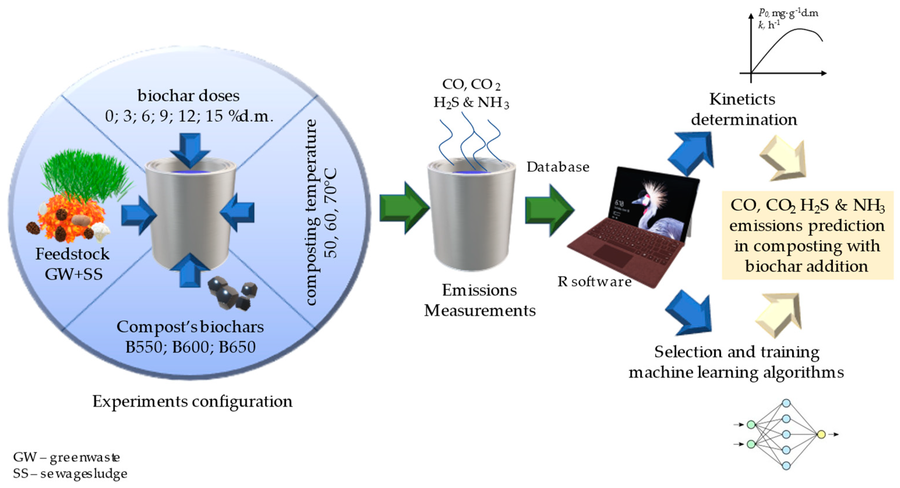
3 emissions during the early stages of laboratory composting. The composting experiments used aa feedstock mix of 90% green waste and 10% sewage sludge acquired from a composting plant (Best-Eko, Rybnik, Poland). Various biochars (B550; B600; B650), produced at different pyrolysis temperatures, were applied at doses of 0, 3, 6, 9, 12 and 15% d.m., as seen in
Figure 1. The appropriate biochar variant was added to the feedstock, placed in 1L reactors, and kept at 50, 60, or 70°CC in a thermostatic cabinet for 10 days. The concentrations of CO, CO
2, H
2S, and NH
3 were measured daily throughout the composting process and then used to calculate emissions.
2.3. Gas Production Monitoring
During the laboratory composting, everyday gas concentrations of CO, CO2, H2S and NH3 were done. For gas concentration measurements the electrochemical gas portable analyzer was used (Nanosens DP-28 BIO; Wysogotowo, Poland). Concentrations of CO, H2S, and NH3 were determined in ppm in the following ranges: CO 0–2000 ppm (±20 ppm), H2S, NH3 0–1000 ppm (±10 ppm), and CO2 0–100% (±2%). Each measurement lasted 45 s, followed by automatic cleaning of the analyzer.
2.4. Gas Production Kinetics Determination
Data for kinetic analysis were analyzed by excluding the lag-phase [
21]. Nonlinear least squares regression was used to determine the kinetic parameters of CO, CO
2 H
2S & NH
3 production. The 1st-order reaction models were used. Prior research has established that the gathered data aligns well with the proposed model [
22,
23].
The 1st-order reaction equation for CO, CO
2, H
2S or NH
3 production is:
where:
P – total production (CO2, mg·g-1d.m; H2S or NH3 µg·g-1d.m),
P0 – maximum production (CO2, mg·g-1d.m; CO, H2S or NH3 µg·g-1d.m),
k – production (CO, CO2, H2S or NH3) constant rate, (h-1),
t – time, (h).
The
k and
P0, calculated from nonlinear regression, were used to calculate the average production or consumption rate (
r) of CO, CO
2, H
2S or NH
3 according to:
where:
r – average production rate (r) of (CO2, mg·g-1d.m; CO, H2S or NH3 µg·g-1d.m),
2.5. Data Pre-Processing
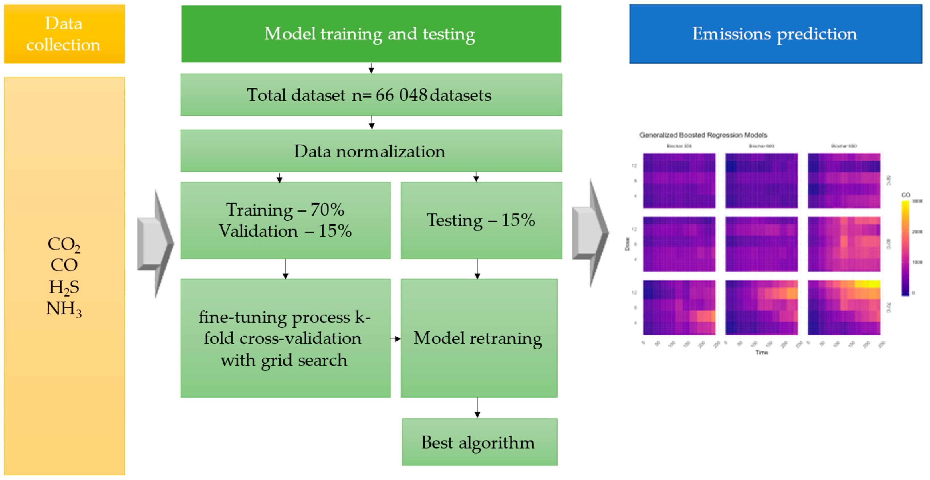
Figure 2 depicts the data processing steps. Initially, 66,048 datasets without missing data were extracted from the selected references. Subsequently, the collected data was normalized from 0 to 1 using Z-Score normalization. Finally, the dataset was randomly divided into training and testing datasets to enhance prediction accuracy, as previously reported [
24]. The data was divided into training/validation/test groups in a 70%/15%/15% proportion. For the fine-tuning process, k-fold cross-validation with grid search was employed. The training dataset assisted in adjusting the hyperparameters and enhancing the prediction abilities of the model, while the testing dataset was used to evaluate the performance of the model and select the appropriate model by comparing the RMSE and R
2 values [
25].
2.6. Selection ML Model Selection and Training Machine Learning Algorithms Evaluation
In this study, ten learning algorithms were evaluated, including both machine set learning and non-set learning. To assess the viability of machine learning methods in the prediction of CO, CO
2, H
2S and NH
3 emissions during the first stage of composting various classes of methods were compared: Linear Models, Tree-Based Models (also part of Ensemble Methods), Support Vector Machines (SVM) and Neural Networks. Calculations were performed using R for Windows [
26] (ver 4.3.2, Vienna, Austria) with caret [
27] and h2o [
28] libraries. The data used for model training related to CO, CO
2, H
2S, and NH
3 emissions from composting, which were obtained from published studies. To predict each gas emission (CO, CO
2, H
2S, and NH
3) individually, principal component analysis (PCA) was conducted to exclude irrelevant parameters. The PCA analysis indicated that observed emissions have a significant correlation and the. The use of other parameters is not justified. PCA (which is a linear dimensionality reduction algorithm) facilitated dimensions standardization and reduction of the initial complexity of the model. Moreover, it will be easier to apply the model in practice if the variables are limited to those that can be easily and cheaply implemented in composting i.e., gas emissions (
Supplementary Materials Figure S1). In model training and prediction, the output and input of the model were the data about CO, CO
2, H
2S, and NH
3 emissions. During the training, when one gas emission was used as an output, the data about the other emissions were utilized as input.
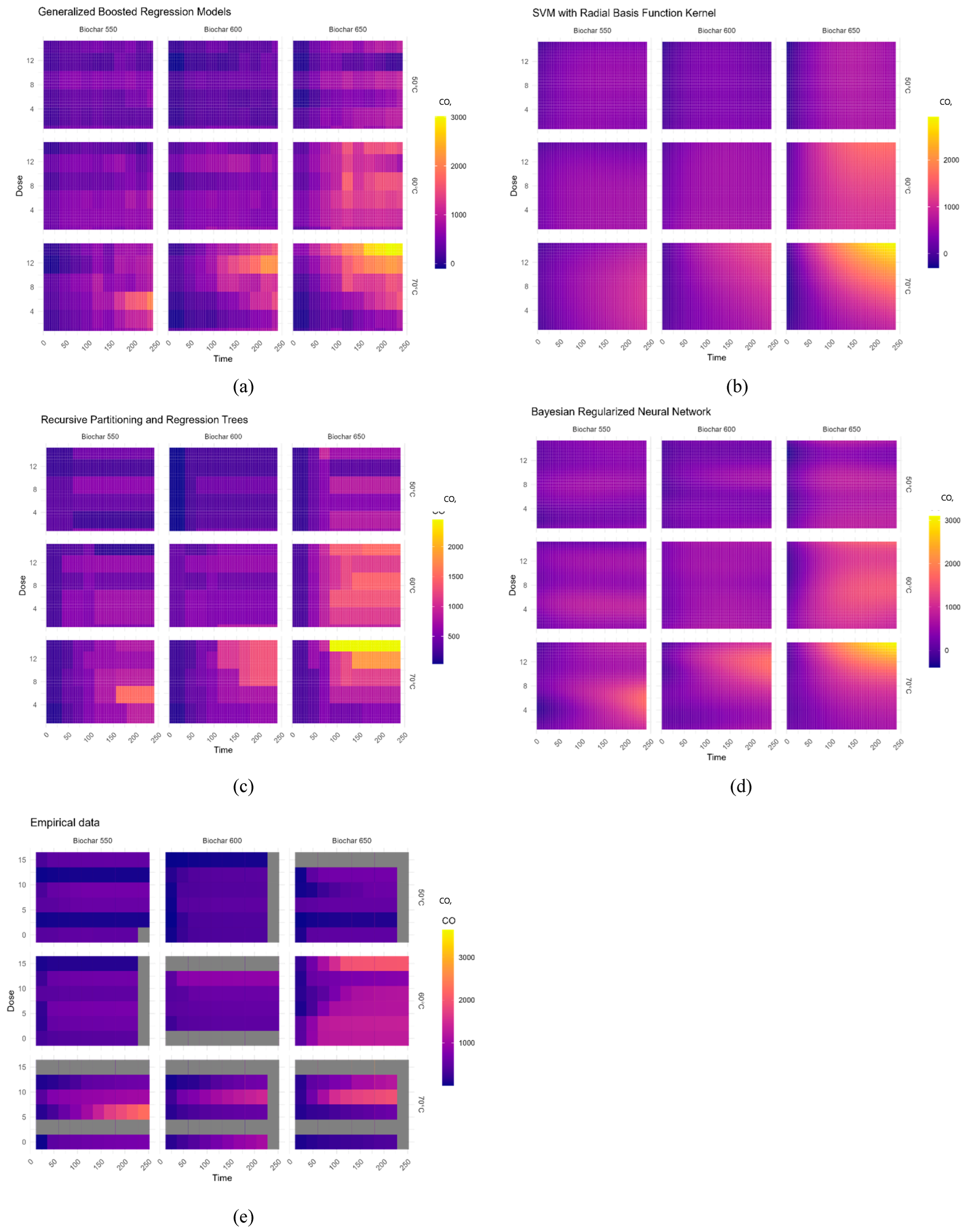
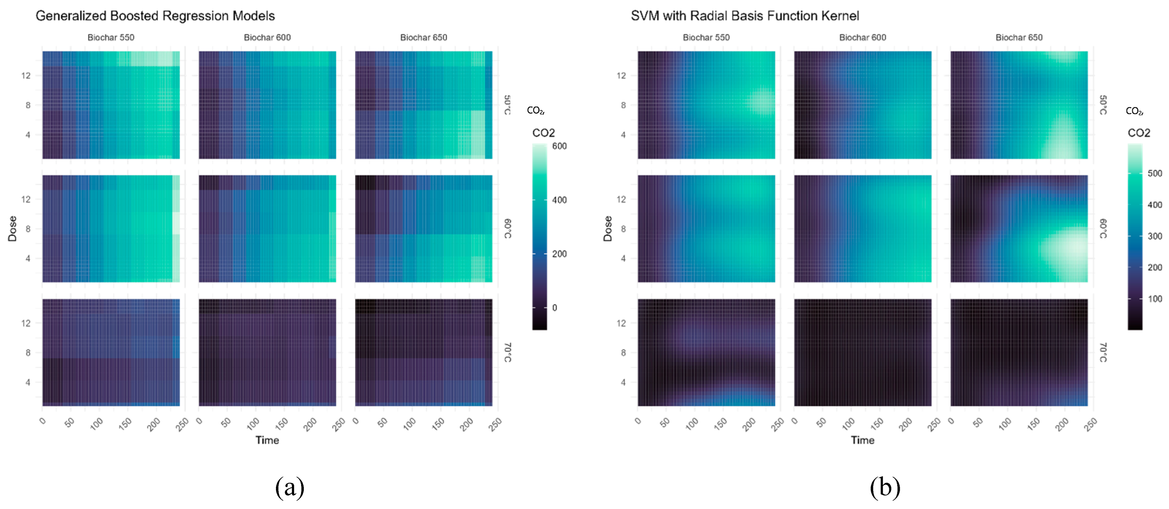
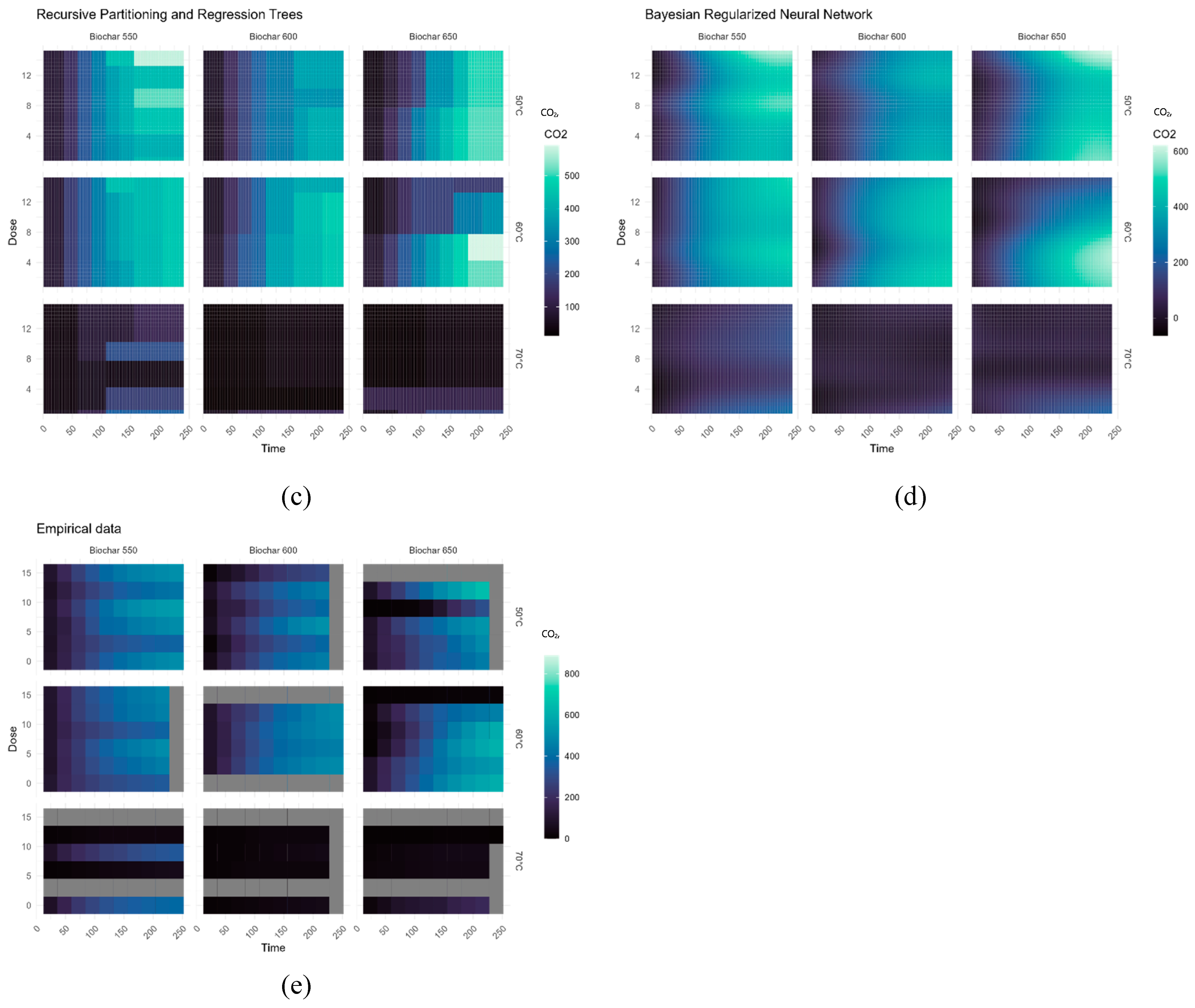
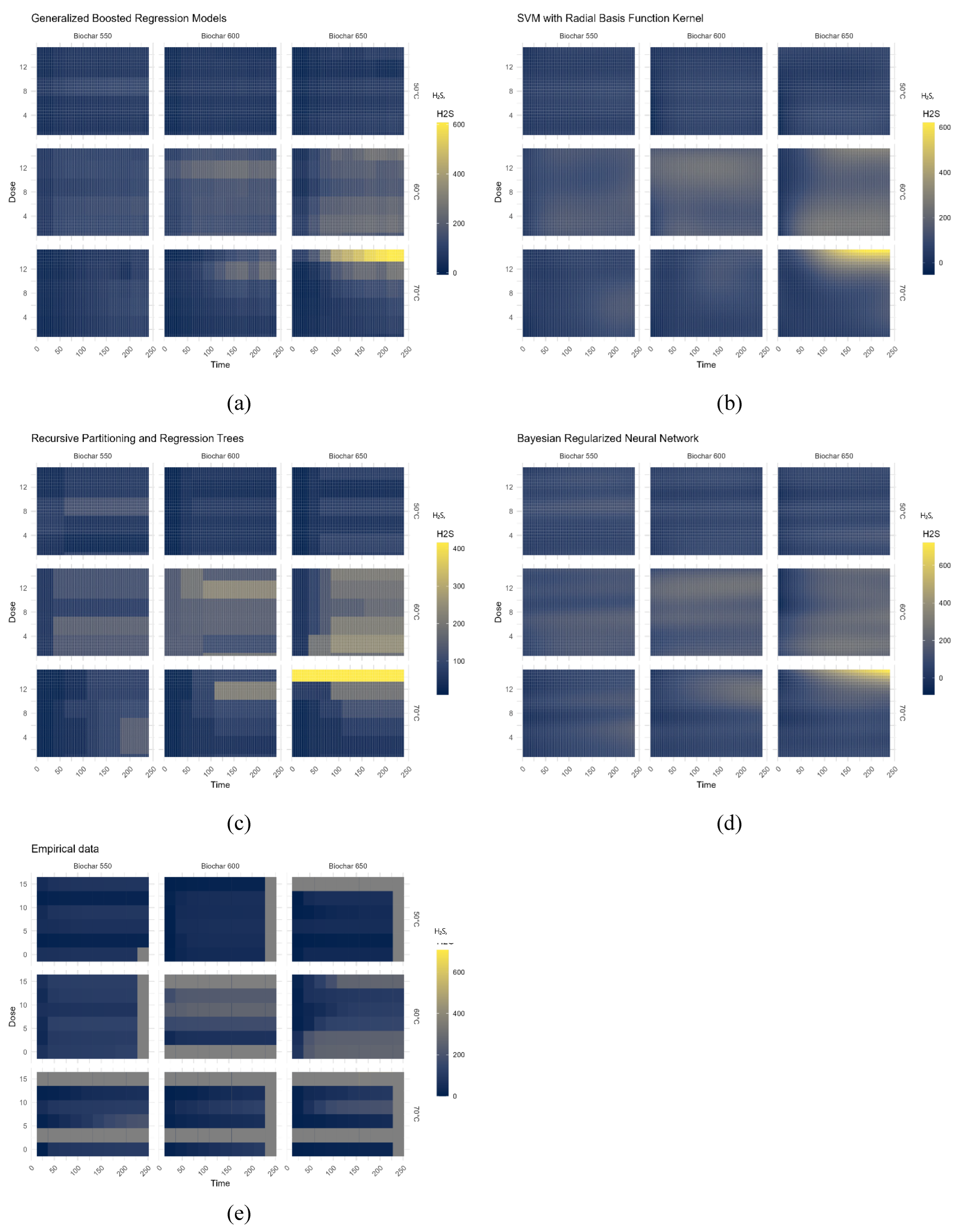
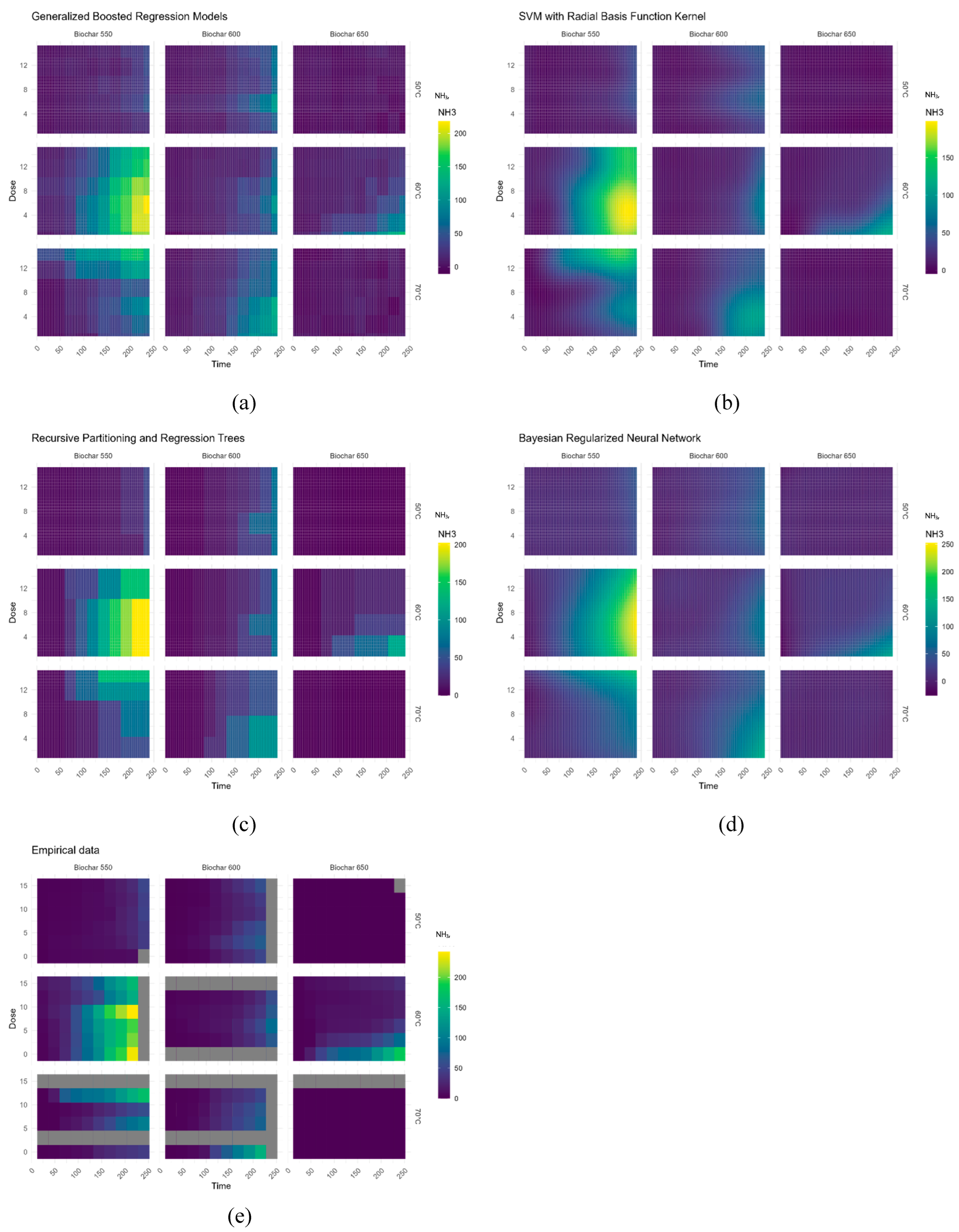
The top four models (Generalized Boosted Regression Models (GBM); SVM with Radial Basis Function (RBF) Kernel Nearest Neighbor Models; Bayesian Regularized Neural Network; Recursive Partitioning and Regression Trees) were depicted as heatmaps, revealing the impact of the four variables: biochar dose, biochar type, incubation temperature, and time on gas emission. Finally, the predicted emissions were compared to the actual emissions to determine the models’ accuracy.
2.7. VOS Viewer Network Map
The VOS viewer software was used to create a network map to analyze the co-occurrence of important for this study keywords. The map’s occurrence and link are determined by taking into consideration the relative abundance of each keyword. Notepad was used to prepare a tab-delimited file containing all keywords, including those of low abundance, for bibliographic data of Web of Science. Further, the type of analysis employed was based on the cooccurrence of keywords that the software read as coauthors. Each keyword is depicted by a circle, with the size of the circle proportional to the frequency of occurrence of the corresponding keyword. The relative abundance of the keyword is determined by the radius of the circle, thereby enabling the visualization of the most frequently occurring keywords. The link between the keyword and the relative size is indicated by a curved line.
4. Discussion
Improving the efficiency and quality of composting is the primary issue for sustainable composting. Although composting has many advantages in the treatment of organic waste, there are still many problems and challenges associated with emissions. Various emissions like NH
3, VOCs, and H
2S, as well as greenhouse gases such as CO
2, CH
4, and N
2O are generated during the process of decomposition of organic compounds [
39]. It is understood that emissions released during the composting process are influenced by both the characteristics of the feedstock and the conditions of the process itself. Effective management emissions techniques such as adsorption/optimizing C/N ratios [
40] (for CO
2 reduction), minimizing N losses (for NH
3 reduction) [
41], and improving pile oxygenation [
42] (for H
2S and CO reduction) can help to control these emissions. One promising approach to enhancing composting conditions to reduce listed above emissions involves the use of compost’s biochar in small quantities [
20]. These observations may explain can observed correlations between the emissions (
Supplementary Material Table S1) and support the accuracy of emissions modeling based on other emissions used in this study.
This constatation supports the network analysis (
Figure 11) the use of ML in composting is mainly connected with ANN and the most analyzed parameters are temperature, nitrogen and heavy metals. The compost and biochar have a large number of connections, with mainly emissions like NH
3, N
2O, CH
4 and CO. There is a low connection between biochar compost and machine learning, what’s proof the novelty of this study.
The novel analytical method based on a mathematical model (MM) and, machine learning (ML) model can explore the relationship between different parameters and draw universal conclusions, which was used to predict emissions during green waste composting. Using modeling techniques can significantly decrease costs and expedite the process of implementing new composting practices, especially when compared to laboratory and pilot-scale investigations. This makes it an attractive option for exploring innovative composting methods [
43].
Currently, the research of MM and ML on aerobic composting is still in the early stages. Mathematical models could enhance the initial mixture of biowaste streams and optimal amounts for composting and thereby help to accelerate the process [
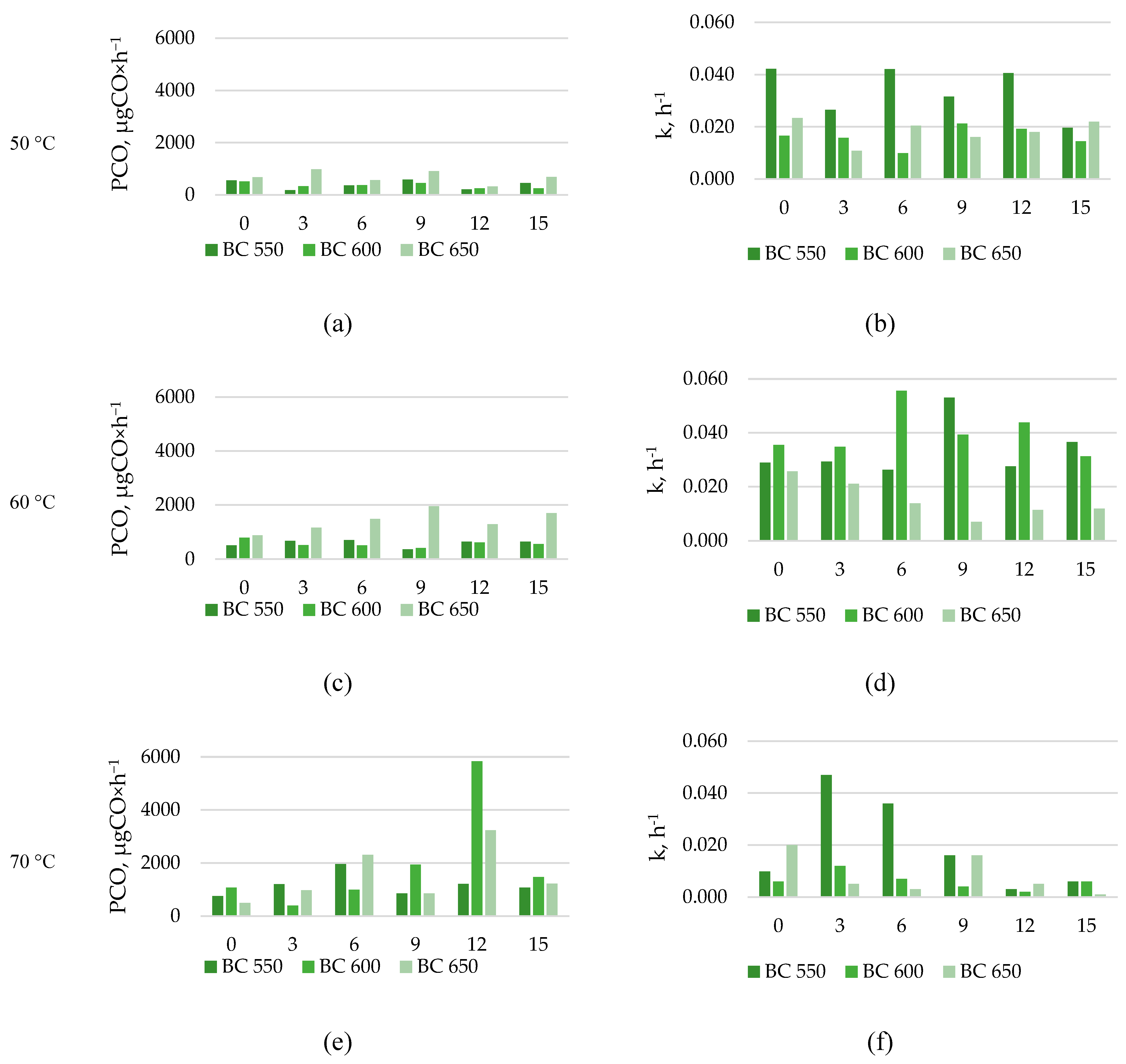
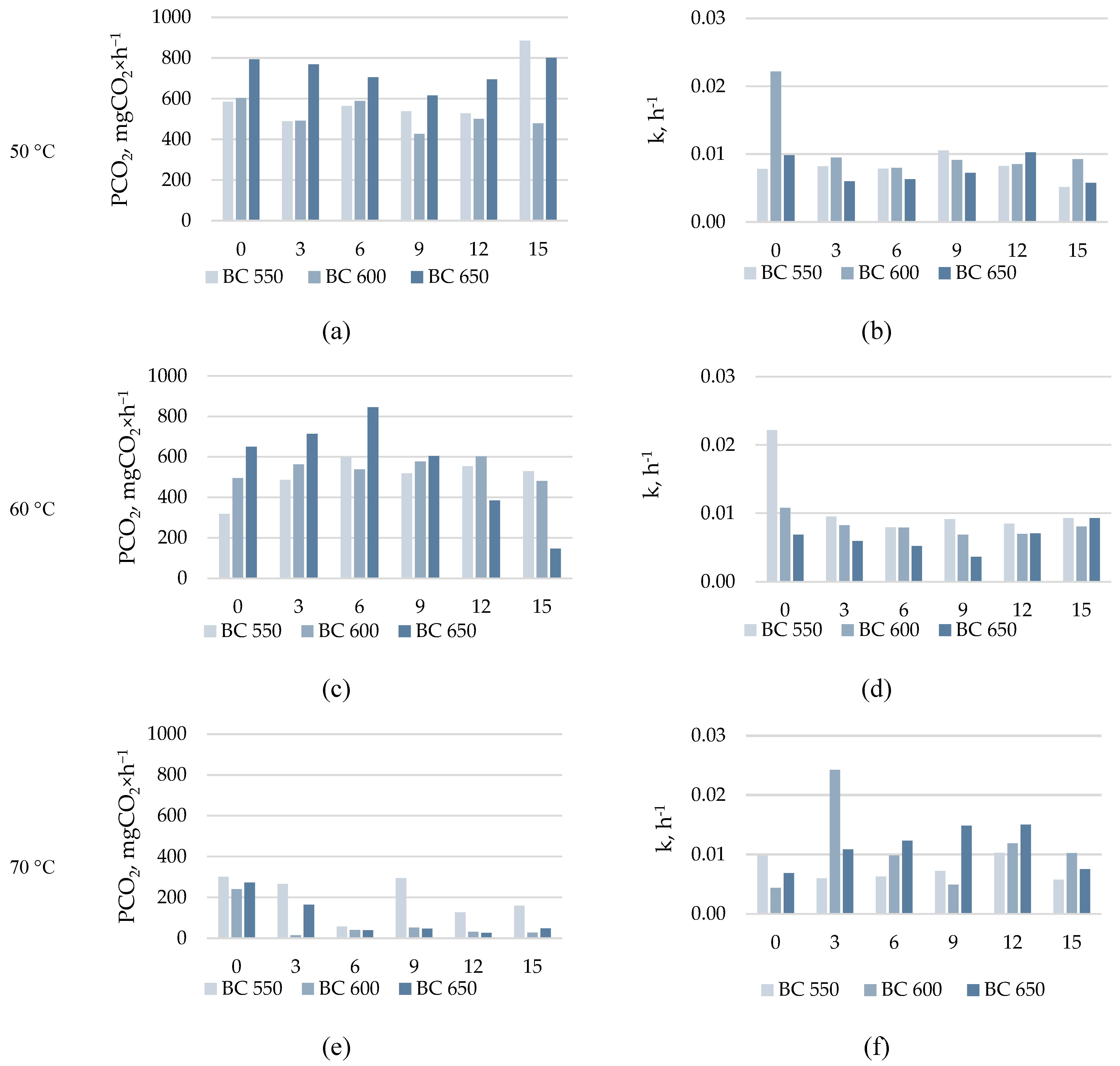
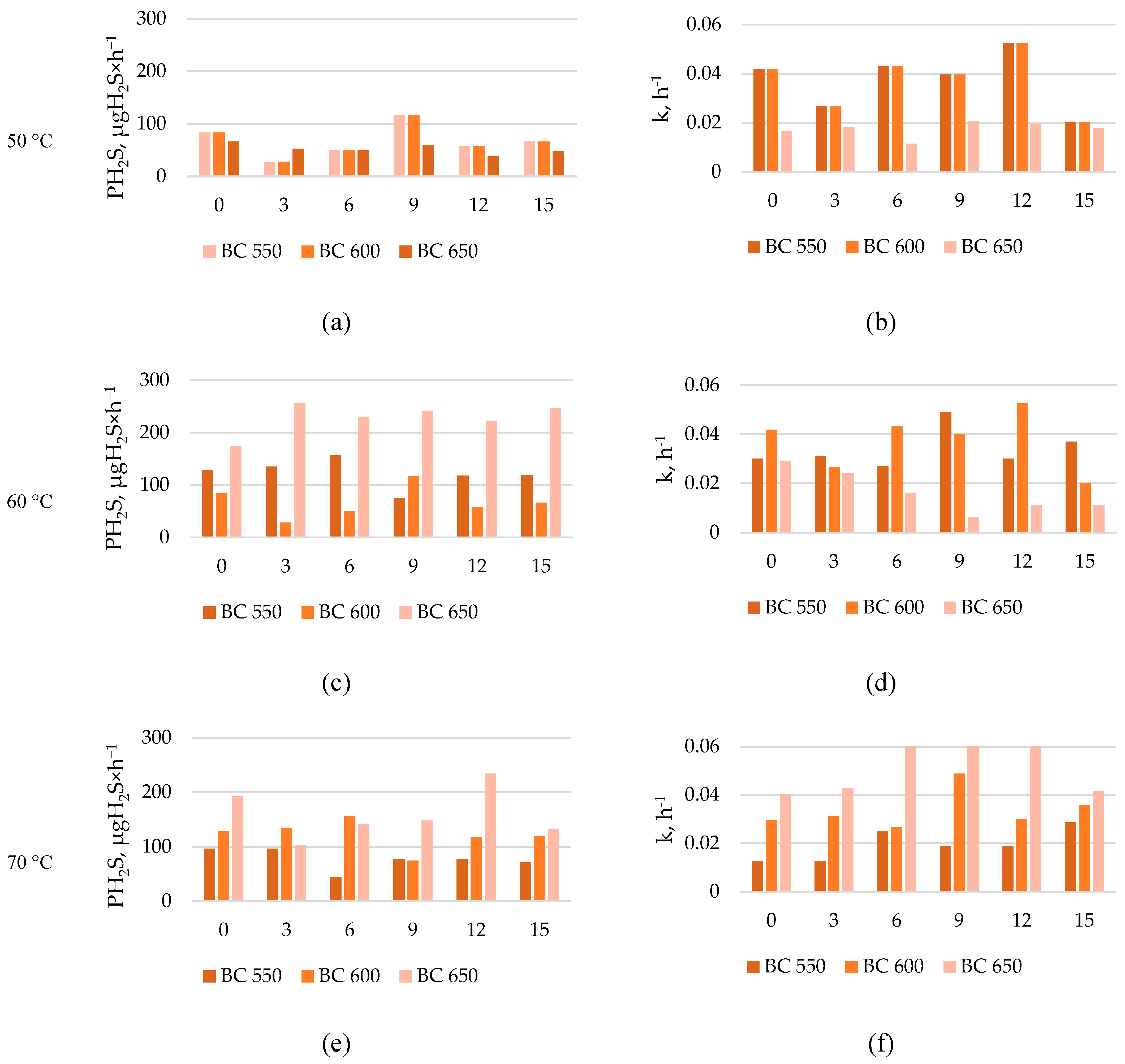
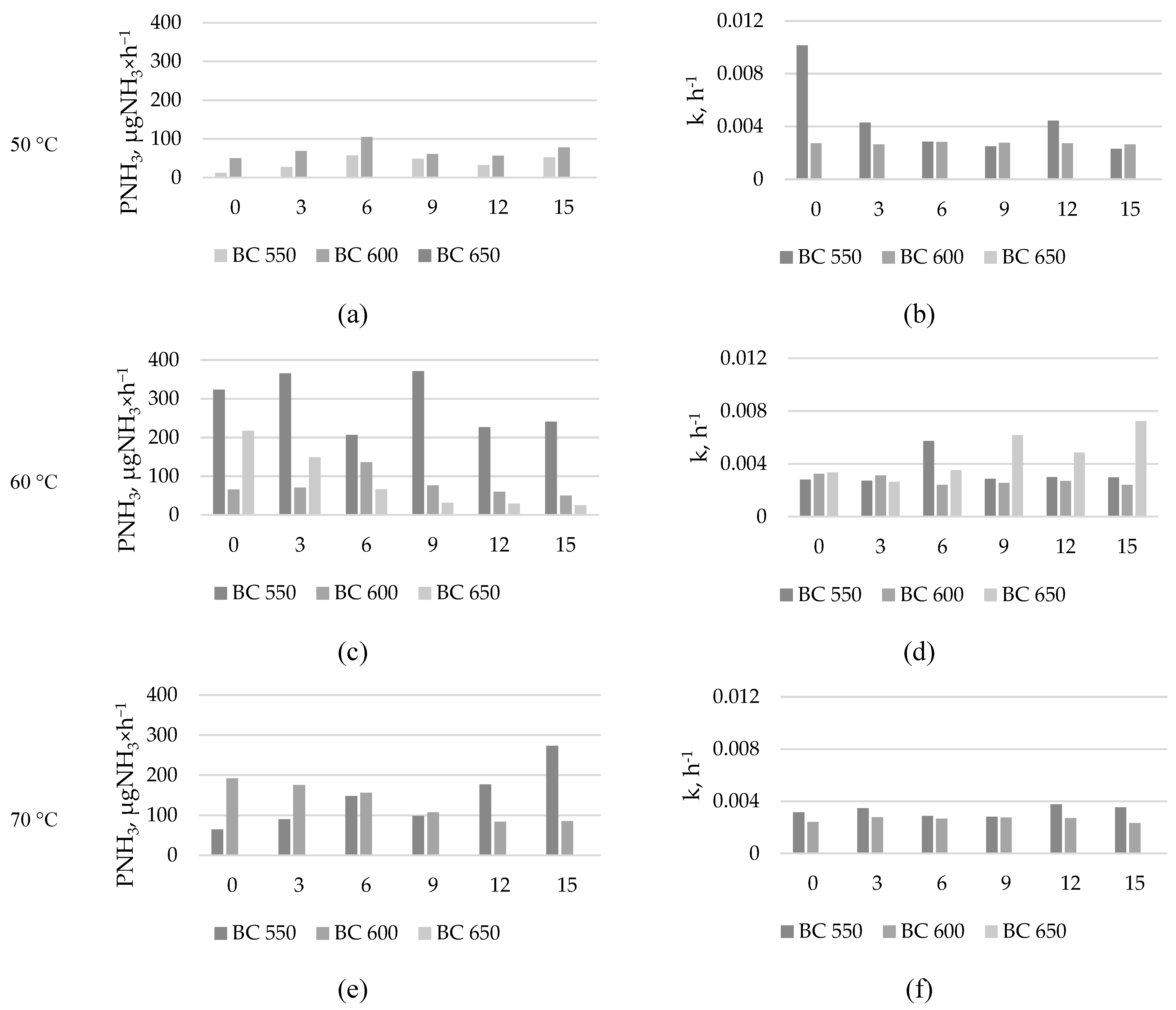
44]. In this study, the first-order kinetics equations were used to estimate the emissions potential during the first 10 days of composting (
Figure 3,
Figure 4,
Figure 5 and
Figure 6,
Supplementary Materials Table S1). The first-order kinetics believed the degradation of organic matter during composting is thought to be enzyme-mediated. The rate of the reaction is determined by the substrate concentration. Mathematical models can be a valuable tool for optimizing process performance in terms of costs, efficiency, and environmental impact by simulating and predicting the process outcome [
45]. Interpretive and optimization methods of MM and ML can be employed to analyze conversion patterns in composting. Previous studies have demonstrated that MM can be utilized to describe the intermediate conversion patterns of biomass, primarily employing empirical equations, Monod-type equations, and first-order kinetics. The first-order kinetic equation is commonly used for composting simulation, but it is less suitable for modeling organics conversion at constant temperature parameters. On the other hand, the first-order has been effectively utilized in estimating the emissions potential from composting. In this study, first-order equations were employed to compare their usefulness with matching learning in the estimation of emissions in composting. In previous research, R
2 was primarily 0.8-0.9 for CO
2 and CO [
22]. However, in this study, it was much lower at 0.5-0.9 (
Supplementary Materials Table S1). For other emissions (H
2S and NH
3), the first kinetic equations effect in wide range fit value – R
2 0.1-0.9 (
Supplementary Materials Table S1). As mentioned above the addition of biochar to composting effecting in change in its properties. This implies that the addition of biochar to compost, alters the emissions production patterns, and mechanism-derived mathematical models may no longer be sufficient.
These observations made the authors focus on predicting the composting process using ML. As shown so far, an ML in composting focuses mostly on predicting the compost maturity and compost properties i.e., pH, EC, GI, TN, TOC, etc, with only a few papers concerned with emissions [
46]. The accuracy of ML models used in composting process prediction changed in the range of 0.56-0.99 for R
2, but in most cases showed good fit >0.7. Common ML models used in composting are as follows: Random Forest (RF), Artificial Neural Network (ANN), Support Vector Regression (SVR), Decision Tree, and Decision Support (DS). RF and ANN are observed to have the best prediction performance, and the accuracy of R
2 was usually > 0.9. In comparison to this study, the best ML models were also ANN (Bayesian Regularized Neural Network), and DT (RPART).
There is a limited number of authors who concentrate on precise forecasts of CO
2 or NH
3 emissions from feedstock composting. Furthermore, no research centers on the anticipation of CO or H
2S during composting using machine learning techniques. Li. et. al. used various ML models to predict CO
2 emissions based on input variables such as TOC, TN, C/N ratio, cellulose, hemicellulose, and lignin. The different models had varying levels of RMSE, with AdaBoost at 49.8, Bagging at 80.6, Gradient Boost at 99.9, Random Forest at 83.0, KNN at 55.0, and Decision Tree at 101.8. These results are similar to ours, as shown in
Table 1. Li et al. found the highest R
2 score of 0.88 accuracy for Random Forest. Bayesian Regularized Neural Network had the best accuracy of 0.81 in the study, while RF achieved an R
2 score of 0.74 for CO
2 emissions production. This indicates that further research should explore the potential of this type of ML model. In other study for predicting NH
3 emissions during composting sewage sludge with straw, Artificial Neural Network (ANN) was utilized. The ANN achieved an R
2 score of over 0.97 by using temperature, pH, EC, C/N, and N-NH4 as input parameters [
47].
The findings of this study suggest that controlling gaseous emissions from green waste composting with compost’s biochar can be achieved by monitoring the emissions of other gases e.g., CO2 output from composting is controllable by CO, H2S, and NH3 emissions. It is important to note that the experimental data used in this study are based on the observations from previous publications and may not fully reflect the control of CO, CO2, H2S and NH3 emissions from composting. Nevertheless, this solution can provide valuable insights for future studies and practices with a larger dataset (especially collected in field study) and more sophisticated ML techniques.
4. Conclusions
This study utilized mathematical models (MM) and machine learning (ML) models to predict the emissions (CO, CO2, H2S, NH3) during first 10 days of composting with compost’s biochar addition. For the first time the ML models to predict CO and H2S during composting were demonstrated. MM has not been very effective in predicting emissions, (R2 0.1 - 0.9), while ML models such as acritical neural network (ANN) and decision tree (DT) have demonstrated satisfactory results. A quality assessment of the developed ML models has shown that the best predictive capacity was reached for ANN (Bayesian Regularized Neural Network; R2 accuracy CO:0,71, CO2:0,81, NH3:0,95, H2S:0,72) and DT (RPART; R2 accuracy CO:0,693, CO2:0,80, NH3:0,93, H2S:0,65). Further research in a semi-scale and field study composting with biochar is also needed to improve the accuracy of development models. In conclusion, this study provided new insights into the enhancement of the composting emissions process.
Figure 1.
Experiments configurations.
Figure 1.
Experiments configurations.
Figure 2.
Machine learning flowchart for predicting emissions from composting with biochar addition.
Figure 2.
Machine learning flowchart for predicting emissions from composting with biochar addition.
Figure 3.
Estimated maximum CO production (µg·g−1 d.m.), and production constant rate (h−1), during the different temperature incubations, biochar type, and biochar dose, a) maximum CO production at 50 °C, b) CO production constant rate at 50 °C, c) maximum CO production at 60 °C, d) CO production constant rate at 60 °C, e) maximum CO production at 70 °C, f) CO production constant rate at 70 °C.
Figure 4.
Estimated maximum CO2 production (mg·g−1 d.m.), and production constant rate (h−1), during the different temperature incubations, biochar type, and biochar dose a) maximum CO2 production at 50 °C, b) CO2 production constant rate at 50 °C, c) maximum CO2 production at 60 °C, d) CO2 production constant rate at 60 °C, e) maximum CO2 production at 70 °C, f) CO2 production constant rate at 70 °C.
Figure 5.
Estimated maximum H2S production (µg·g−1 d.m.), and production constant rate (h−1), during the different temperature incubations, biochar type, and biochar dose, a) maximum H2S production at 50 °C, b) H2S production constant rate at 50 °C, c) maximum H2S production at 60 °C, d) H2S production constant rate at 60 °C, e) maximum H2S production at 70 °C, f) H2S production constant rate at 70 °C.
Figure 6.
Estimated maximum NH3 production (µg·g−1 d.m.), and production constant rate (h−1), during the different temperature incubations, biochar type, and biochar dose, a) maximum NH3 production at 50 °C, b) NH3 production constant rate at 50 °C, c) maximum NH3 production at 60 °C, d) NH3 production constant rate at 60 °C, e) maximum NH3 production at 70 °C, f) NH3 production constant rate at 70 °C.
Figure 7.
Predicted CO production (µg·g−1 d.m.) based on biochar temperature production, incubation temperature and dose of biochar, using a) Generalized Boosted Regression Models °C, b) SVM with Radial Basis Function Kernel, c) Recursive Partitioning and Regression Trees, d) Bayesian Regularized Neural Network, e) Empirical data.
Figure 8.
Predicted CO2 production (mg·g−1 d.m.) based on biochar temperature production, incubation temperature and dose of biochar, using a) Generalized Boosted Regression Models °C, b) SVM with Radial Basis Function Kernel, c) Recursive Partitioning and Regression Trees, d) Bayesian Regularized Neural Network, e) Empirical data.
Figure 9.
Predicted H2S production (µg·g−1 d.m.) based on biochar temperature production, incubation temperature and dose of biochar, using a) Generalized Boosted Regression Models °C, b) SVM with Radial Basis Function Kernel, c) Recursive Partitioning and Regression Trees, d) Bayesian Regularized Neural Network, e) Empirical data.
Figure 10.
Predicted NH3 production (µg·g−1 d.m.) based on biochar temperature production, incubation temperature and dose of biochar, using a) Generalized Boosted Regression Models, b) SVM with Radial Basis Function Kernel, c) Recursive Partitioning and Regression Trees, d) Bayesian Regularized Neural Network, e) Empirical data.
Figure 11.
Network analysis of co-occurrence of important keywords.
Figure 11.
Network analysis of co-occurrence of important keywords.
Table 1.
Comparisons between particular models by values of R squared and RMSE.
Table 1.
Comparisons between particular models by values of R squared and RMSE.
| Model |
CO |
CO2
|
NH3
|
H2S |
| R2
|
RMSE |
R2
|
RMSE |
R2
|
RMSE |
R2
|
RMSE |
| Linear Regression |
0.304 |
376.870 |
0.538 |
120.130 |
0.350 |
36.010 |
0.141 |
83.533 |
| Random Forest |
0.463 |
331.256 |
0.741 |
89.841 |
0.918 |
12.791 |
0.567 |
59.277 |
| SVM with Linear Kernel |
0.255 |
389.928 |
0.503 |
124.443 |
0.212 |
39.644 |
0.072 |
86.811 |
| SVM with RBF Kernel |
0.636 |
272.579 |
0.776 |
83.699 |
0.900 |
14.125 |
0.602 |
56.888 |
| k-Nearest Neighbors |
0.466 |
330.187 |
0.730 |
91.852 |
0.895 |
14.453 |
0.261 |
77.461 |
| Bayesian Regularized Neural Network |
0.710 |
243.318 |
0.808 |
77.465 |
0.948 |
10.159 |
0.715 |
48.111 |
| RPART |
0.693 |
250.324 |
0.802 |
78.562 |
0.930 |
11.796 |
0.648 |
53.459 |
| Generalized Boosted Regression Models |
0.595 |
287.527 |
0.764 |
79.493 |
0.899 |
14.163 |
0.584 |
58.104 |
| Extreme Gradient Boosting Tree |
0.309 |
375.754 |
0.798 |
85.764 |
0.793 |
20.326 |
0.486 |
64.608 |
| Partial Least Squares Regression |
- |
- |
0.544 |
119.348 |
0.360 |
35.737 |
0.149 |
83.131 |
