A Streaming Algorithm for a Fast, Robust, and Memoryless Median Estimation on Sensor Data

Preprint

Article

A Streaming Algorithm for a Fast, Robust, and Memoryless Median Estimation on Sensor Data

Altmetrics

Downloads

Views

Comments

This version is not peer-reviewed

Submitted:

27 April 2024

Posted:

29 April 2024

You are already at the latest version

Alerts

Abstract

We propose a novel moving median estimator specifically designed for online detection of threshold crossings in multi-channel signals, such as extracellular neural recordings. This estimator offers two key advantages: a reduced sensitivity to outliers and the elimination of memory requirements for storing arrival times. Furthermore, its design facilitates parallel implementation on FPGAs, making it ideal for real-time processing of multi-channel recordings.

Keywords:

Subject: Computer Science and Mathematics - Probability and Statistics

1. Introduction

Median filtering is a widely used technique to remove or detect infrequent events in signal and image processing. Depending on what part of the raw signal is removed, the median filter can be employed to eliminate or to capture impulse noise from signals and images [1], as in the case of extracellular neuronal spikes or “pepper and salt” noise, respectively.

When those few frequent events are contaminated with Gaussian noise, as in the case of extracellular neuron recordings, an optimal threshold can be calculated to separate spikes from noise [2]. Indeed, most of the state-of-the art neuronal decoding techniques starts with threshold-based spikes detection, independently of what kind of analysis is done after this stage, i.e. multiunit or single unit spike sorting isolation decoding [3,4,5].

While it is straightforward to compute the median-based threshold in offline spike detection analysis, limitations related to speed and memory appear in real time neuronal decoding of multichannel recordings, mainly due to the huge amount of samples per seconds that arrive from the recording equipment and the non-stationary characteristics of those signals. In consequence, to have a fast and accurate real-time median-driven threshold estimator becomes critical.

In digital systems, sample median computations relies in sorting methods, which are a special case of selection algorithms. In an ordered odd buffer, the buffer middle sample results in the median of those samples. Thus, improving the efficiency of the sample ordering process impacts directly in the estimation speed,

N \cdot log (N)

[6].

In a moving (sliding window) median estimator, as soon as the window moves over a new sample, two alternatives can be used in order to estimate the new buffer median value, a naive one that implies to re-order the whole buffer as if it were a new and independent set of samples, or a more efficient one that results from dropping out the oldest sample in the buffer and inserting the new one in such a position that keep the buffer ordered. While the former affects the speed of median estimation, the latter need to keep in memory the temporal order in which every sample arrived to the buffer, requiring as many memory as positions in the buffer exist.

We present here an alternative method to compute the median in sliding windows and, in consequence, the optimal moving threshold to detect impulse noise from Gaussian one. The method avoids keeping in memory the order the sample arrival without re-ordering the whole buffer every time a sample comes in. We demonstrate that the proposed method is unbiased and robust compared to the traditional moving median, particularly when the underlying process is stationary. Furthermore, it adapts to a new sample distribution in at most 1.5 times the time required by the traditional method during significant shifts in the signal baseline, such as those encountered in extracellular recordings due to electrode movements.

2. Methods

Let

X (t)

be a continuous random process, with probability distribution density function

f_{X} (x)

, which we will only assume it is uni-modal. The classical moving median estimator can be computed, at time

t_{n}

μ_{t_{n}} = m e d i a n {x_{t_{n}}, x_{t_{n - 1}}, . . ., x_{t_{n - (L - 1)}}}

(1)

when using a buffer of length L.

A naive implementation for estimating a moving median requires tracking both the order of sample arrivals and sorting the entire buffer (window) each time a new sample is received, resulting in an algorithmic complexity of

O (N^{2})

. A more efficient approach involves maintaining a sorted copy of the window data, allowing for the insertion of new samples into their correct positions while simultaneously deleting the oldest element in the buffer and appropriately shifting the remaining samples. With this method, originating from an ordered buffer, the complexity diminishes to

O (N log N)

operations on average. However, it demands maintaining the history of sample arrivals to the buffer, which proves both memory and time-intensive. In real-time implementations, this poses a new challenge: ensuring that the output keeps pace with the input data rate to prevent data loss.

We propose a novel real-time median estimator where the new incoming samples are inserted into the buffer in an orderly fashion. In our algorithm, instead of discarding the oldest sample, we suggest removing a sample at the extremity of the buffer that is farthest from the new sample.

Given a buffer B with L positions (

{B_{1}, . . ., B_{L}}

), being L odd and

m = (L - 1) / 2

B (m)

is the element in the middle of the buffer, the update rule for a new sample x is:

(a) if x < B(m) then,

if exists k / x > B(k) with k < m then,

B=[B(1), B(2), ..., B(k), x, B(k+1), ..., B(m), ..., B(L-1)]

else

B=[x, B(1), ..., B(m), ..., B(L-1)]

(b) else if x > B(m) then,

if exists k / x < B(k) with k>m then,

B=[B(2), ..., B(m), ..., B(k-1), x, B(k), ..., B(L)]

else

B=[B(2), ..., B(m), ..., B(L), x]

(c) else, (x==B(m))

B=[B(2), ..., B(m), x, ..., B(L)]

or

B=[B(1), ..., x, B(m), ..., B(L-1)]

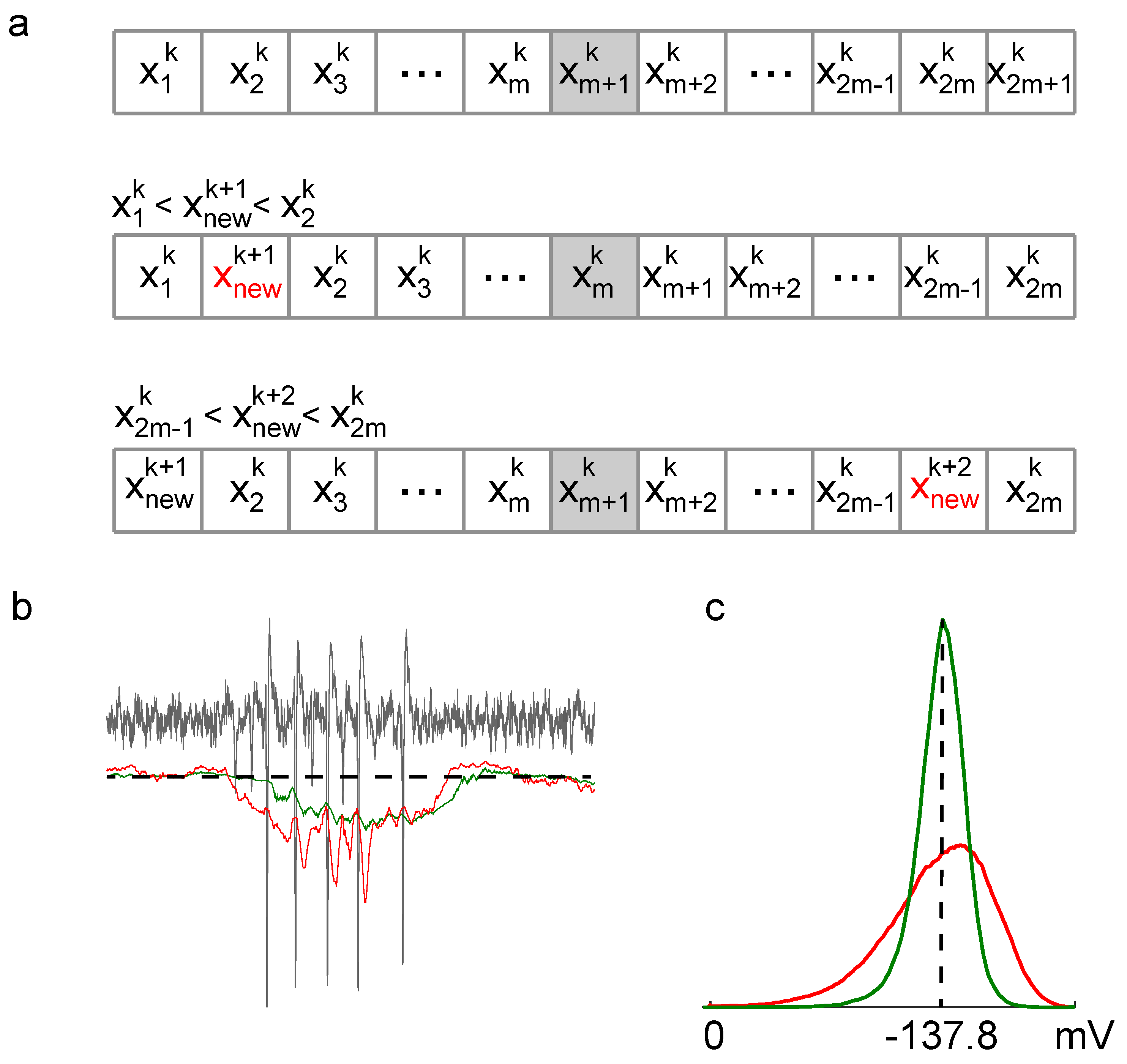
When a new sample x arrives, it can be lower, higher or equal to the element in the center of the buffer

B (m)

. In the first case, two situations can arise: the new sample can be higher than a given element of the buffer

x > B (k)

(and lower than

B (k + 1)

with

k < m

) in which case the new sample is inserted between

B (k)

and

B (k + 1)

, or lower than all the elements of the buffer in which case, the new sample is inserted in the first position of the buffer. In both these cases, the last element of the buffer

B (L)

is dropped. In case the new sample x is higher than

B (m)

, equivalent to the previous situation, the new sample will be inserted in the higher part of the buffer, and

B (1)

will be dropped. Finally, in the case that the new sample is equal to the element in the center of the buffer (

x = B (m)

), either the first element or the last element of the buffer is dropped.

It is important to remark that in this algorithm: a) the elements in the buffer B are consistently sorted, b) the new sample x is always inserted in the buffer, c) There is no requirement for information about the time of sample arrival.

To determine the position where the new element should be inserted, we must either locate an element of the same value in the buffer or conduct at least

O (log (N))

comparisons using a binary search algorithm.

3. Results

While median filtering finds applications in various domains, our focus will be on its application in extracellular neuron spike detection. Electrodes in a multichannel extracellular recording setup can detect abrupt electrical changes in their vicinity. However, they also capture the aggregate of numerous electrical signals originating from distant neuron populations, alongside various electrical artifacts.

Regardless of the individual probability distributions of these punctual sources, the central limit theorem dictates that their collective contribution approximates a normal distribution. Consequently, the stronger the electrical field perturbation caused by a nearby neuron spike on an electrode, the greater the likelihood of discerning it as a single-cell action potential. Thus, it is customary to define the signal-to-noise ratio (SNR) between spikes and background noise as the ratio of the spike peak voltage to the standard deviation of the background noise, denoted as

σ_{n o i s e}

. A SNR value of K indicates that the spike peak voltage is K times the standard deviation of the background noise, denoted as

σ_{n o i s e}

. In the case of Gaussian noise

N (0, σ_{n o i s e}^{2})

, a linear relationship exists between its standard deviation and the median of the half-normal distribution

y = | x |

σ_{n o i s e} = \frac{median \{| x |\}}{\sqrt{2} {e r f}^{- 1} (1 / 2)} \approx \frac{median \{| x |\}}{0.675}

(2)

Thus, computing a threshold T to detect events surpassing T reduces the computation of

σ_{n o i s e}

to the median of

y = | x |

, with

p (x) = N (0, σ_{n o i s e}^{2})

In Figure 1, we present a schematic illustrating the step-by-step insertion of new samples into the buffer and the subsequent discarding of samples according to the algorithm outlined in the methods section. Compared to the classical moving median estimator, the proposed method exhibits a smaller variance when applied to real neuronal extracellular recordings. This reduction in variance translates to fewer missed spikes and eliminates the erroneous detection of non-existent spikes, which is particularly important for accurate spike detection thresholding.

The reduction in variance in the estimation is attributed to the fact that samples are discarded from the buffer based on their position within it, rather than their arrival times. Specifically, in a buffer initially populated with the first L samples in order, the classical moving median (CMM) estimator discards the oldest sample in the buffer each time a new sample arrives, whereas our algorithm (NM) discards a sample from the buffer’s extremity. Intuitively, this can be understood as a compressing process of sample selection, ultimately resulting in a buffer populated with samples closer to the median.

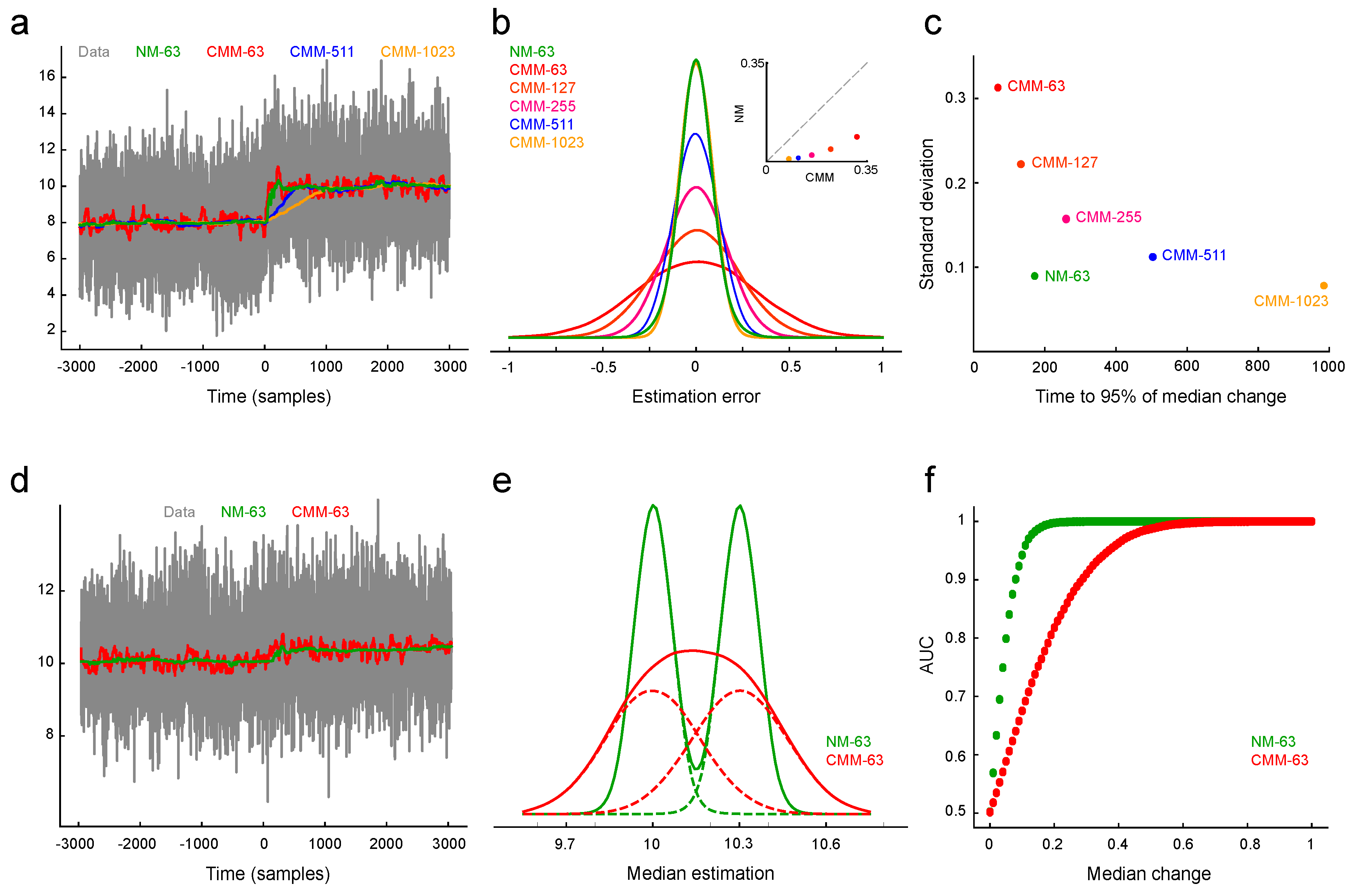
It is noteworthy that the classical algorithm maintains a true sampling distribution of the original signal, while ours does not fully reflect this distribution. We reasoned that while this characteristic may offer an advantage in a stationary process, it may result in a delay in reaching the new median value when a change in the median signal occurs. Furthermore, the delay in reaching the correct estimation of the median and the length of the buffer are also related. Larger buffers indeed offer less dispersion around the real median and provide more stability at the cost of slower responses to process changes. To investigate this phenomenon, we conducted a series of simulations using signals constructed from real recording noise and spikes, with spikes uniformly distributed among the basal noise. Therefore, for a set of buffers with lengths 63, 511, and 1023, we introduced a controlled change in the signal values at time 0 and examined the dynamic changes in the median estimation (see Figure 2).

Unlike the Classical Moving Median (CMM) estimator, where changes are reflected in the estimation within a fixed time window L, our algorithm’s response time depends on the magnitude of the change. For large changes with entirely new samples, our algorithm requires on average between

L / 2

and

3 L / 2

time steps to achieve the same. However, for small changes, the new samples are added to the edges of the buffer and may take longer than L steps to fully influence the estimate due to the discarding process.

To demonstrate the algorithm’s robustness against outliers, we analyzed the sample density dynamics within the buffer over time. To directly compare NM with the CMM algorithm, we initially filled both buffers with L pre-sorted samples. This ensures the NM estimator’s initial distribution reflects the underlying data. However, unlike CMM where this distribution remains constant, the NM estimator continuously compresses the buffer’s sample distribution towards the median value, typically within a few buffer cycles.

We ran the algorithm with a buffer length of L=1023 samples, feeding it data from a normal distribution

N (0, 1)

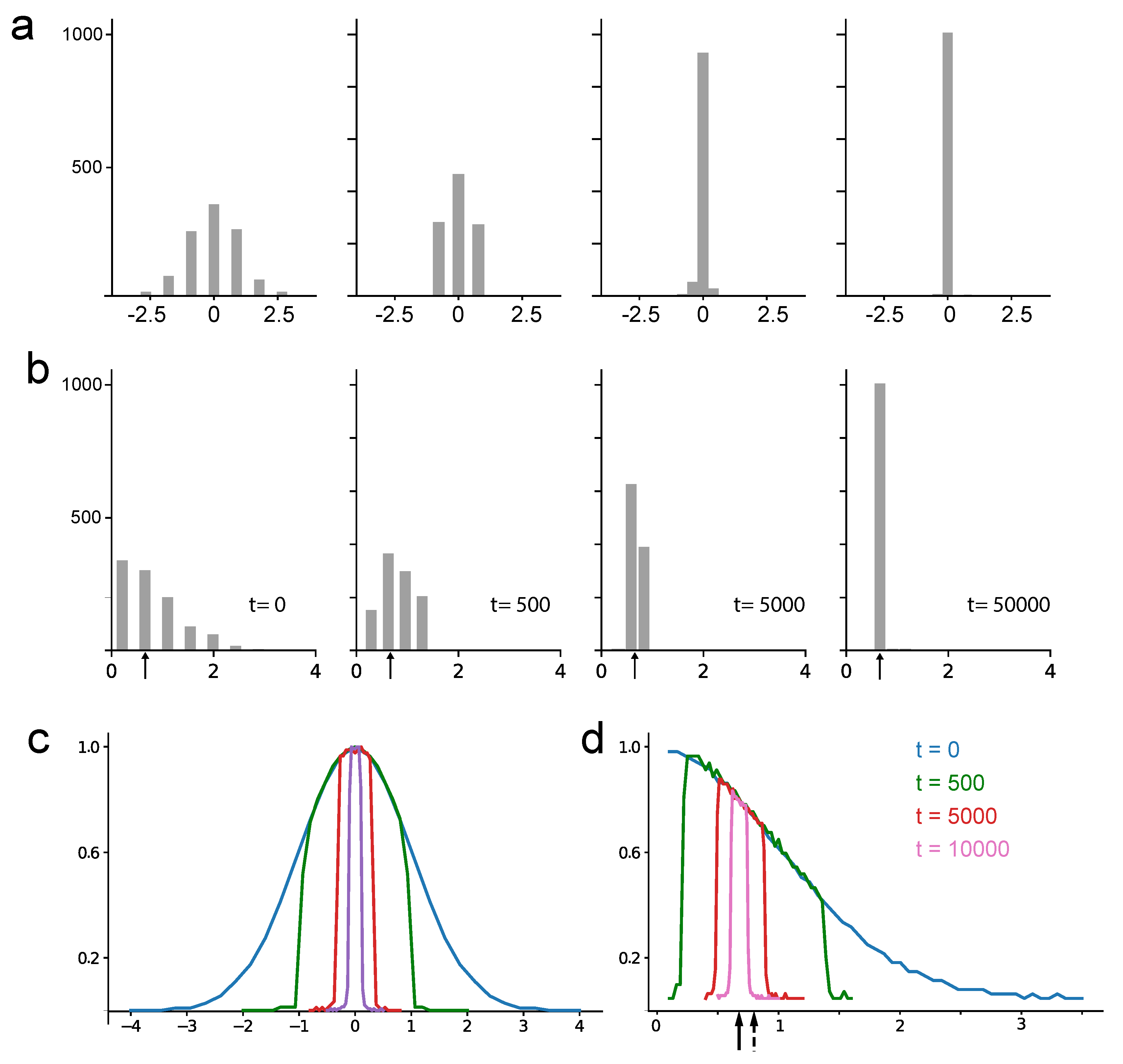
. We then analyzed the sample density within the buffer at different points in time, starting from when the buffer was initially filled. Figure 3a shows these sample density changes. Particularly noteworthy, the initially Gaussian distribution becomes progressively more concentrated around the data’s mean (or median for a normal distribution), approaching a uniform distribution with significantly reduced variance.

We repeated the analysis for a folded normal distribution (the distribution of

| x |

when

x \sim N (0, 1)

. Figure 3b shows the sample distribution within the buffer over time, starting from a buffer completely filled with fresh samples drawn from the folded normal distribution, and continuing up to

50, 000

time steps. This scenario, with a folded normal distribution, is more relevant to real extracellular recordings where the median and mean typically differ. As can be readily observed, the buffer samples distribute around the noise median in this case.

Interestingly, repeating both experiments 10,000 times and averaging their sample distributions across different time points reveals a consistent trend. The average sample distribution concentrates around the median value of the initial distribution, essentially copying its shape. This behavior is evident in Figure 3b for the normal distribution and Figure 3c for the folded normal distribution. Consequently, filling the buffer with values increasingly closer to the true median with each iteration enhances the method’s robustness against outlier perturbations.

By definition, the median m is the value that satisfy

\int_{- \infty}^{m} p (x) d x = \int_{m}^{- \infty} p (x) d x = \frac{1}{2}

(3)

for any other value

m_{x}

different to m we will have

A = \int_{- \infty}^{m_{x}} p (x) d x; B = \int_{m_{x}}^{- \infty} p (x) d x

(4)

with

A \neq B

If the value at the center of the buffer

m_{x}

is less than the true median m, there will be an imbalance. The distribution function,

F (x)

, tells us that there are more samples greater than

m_{x}

than expected

F (m) - F (m_{x}) > 0

. These additional high-value samples on the right side of the buffer tend to push

m_{x}

towards the left. This creates an opportunity for values greater than

m_{x}

to occupy the buffer center position. The opposite happens when

m_{x}

is larger than the true median.

This process can be likened to the diffusion of non-charged particles across a membrane, as described by Fick’s Laws [8]:

J = - D \frac{\partial ϕ}{\partial x}

(5)

where J is the net flux across the membrane, D is the diffusion coefficient (

D = 1

here) and

\frac{\partial ϕ}{\partial x}

is the concentration difference across the membrane.

The process reaches equilibrium, indicated by a zero net flux of zero particles across the membrane, when the concentration of particles on both sides becomes equal. In simpler terms, this occurs when the same proportion of samples are found above and below the central value,

A = B = 1 / 2

, which occurs when

m_{x}

itself equals the true median m.

By exploiting this natural dynamic, our algorithm achieves an unbiased estimation of the signal’s median under stationary conditions.

4. Discussion

There are two main categories of quantile estimators: those that calculate the statistics using the entire dataset and those that rely on a subset of the data.

There is a significant amount of research on computing median estimators in data streams, specifically to be applied to filtering techniques. These techniques often involve calculating the exact median of a window containing L samples and then using this value to estimate an appropriate threshold.

On the other hand, quantile estimation is a powerful technique for characterizing dataset properties. It enables the online estimation of various order statistics, including the minimum, maximum, median, quartiles, and any other quantiles (q-quantile).

In streaming algorithms, finding the minimum and maximum values only requires

O (1)

operations, while estimating the median requires at least

O (l o g L)

operations [9,10]. Efficient online computation of quantile statistics are mainly based on the work of Greenwald and Khanna [11,12]. These algorithms are designed to maintain statistics of arbitrary quantiles. While they are efficient in terms of memory usage and have optimal complexity performing order

O (1)

operations, these operations are not suitable for implementation on field-programmable logic arrays (FPGAs). FPGAs are often preferred for their low-power and high-performance capabilities in real-time applications, making them unsuitable for these specific algorithms. Consequently, the complexity and computational cost of implementing them outside of a traditional computer or embedded system are very high.

Although the proposed method is limited to estimating the median, its implementation on FPGAs for this specific task is remarkably straightforward. This efficiency stems from the fact that it only requires basic operations like comparisons and shifting, which are highly optimized for FPGAs and GPUs. Furthermore, it boasts a complexity of O(log L) when starting from an already sorted buffer.

Author Contributions

A.B., J.S.C. and S.E.L contributed equally to manuscript preparation. All authors have read and agreed to the published version of the manuscript.

Funding

This research was funded by Universidad de Buenos Aires, UBACyT 20020220200032BA.

Data Availability Statement

The original contributions presented in the study are included in the article, further inquiries can be directed to the corresponding author.

Conflicts of Interest

The authors declare no conflicts of interest.

Abbreviations

The following abbreviations are used in this manuscript:

CMM	Classical Moving Median
FPGA	Field Programmable Gates Arrays
GPU	Graphics Processing Unit
NM	New Median
SNR	Signal to Noise Ratio

References

Ibrahim, H.; Pik Kong, N.S.; Ng, T.F. Simple Adaptive Median Filter for the Removal of Impulse Noise from Highly Corrupted Images. IEEE Transactions on Consumer Electronics 2008, 54, 1920–1927. [Google Scholar] [CrossRef]
Donoho, D. De-Noising by Soft-Thresholding. IEEE Transactions on Information Theory 1995, 41, 613–627. [Google Scholar] [CrossRef]
Stark, E.; Abeles, M. Predicting Movement from Multiunit Activity. Journal of Neuroscience 2007, 27, 8387–8394. [Google Scholar] [CrossRef]
Flint, R.D.; Wright, Z.A.; Scheid, M.R.; Slutzky, M.W. Long Term, Stable Brain Machine Interface Performance Using Local Field Potentials and Multiunit Spikes. Journal of Neural Engineering 2013, 10, 056005. [Google Scholar] [CrossRef] [PubMed]
Quiroga, R.; Nadasdy, Z.; Ben-Shaul, Y. Unsupervised Spike Detection and Sorting with Wavelets and Superparamagnetic Clustering. Neural Computation 2004, 16, 1661–1687. [Google Scholar] [CrossRef]
Hoare, C.A.R. Algorithm 64: Quicksort. Communications of the ACM 1961, 4, 321. [Google Scholar] [CrossRef]
Mininni, C.J.; Caiafa, C.F.; Zanutto, B.S.; Tseng, K.Y.; Lew, S.E. Putative Dopamine Neurons in the Ventral Tegmental Area Enhance Information Coding in the Prefrontal Cortex. Scientific Reports 2018, 8, 11740. [Google Scholar] [CrossRef] [PubMed]
Fick, A. On liquid diffusion. The London, Edinburgh, and Dublin Philosophical Magazine and Journal of Science 1885, 10, 30–39. [Google Scholar] [CrossRef]
Ivkin, N.; Liberty, E.; Lang, K.; Karnin, Z.; Braverman, V. Streaming Quantiles Algorithms with Small Space and Update Time. Sensors 2022, 22, 9612. [Google Scholar] [CrossRef] [PubMed]
Raykov, P. An Optimal Algorithm for Sliding Window Order Statistics. 26th International Conference on Database Theory (ICDT 2023). Schloss Dagstuhl – Leibniz-Zentrum für Informatik, 2023. [CrossRef]
Greenwald, M.; Khanna, S. Space-Efficient Online Computation of Quantile Summaries. ACM SIGMOD Record 2001, 30, 58–66. [Google Scholar] [CrossRef]
Liang, C.; Li, M.; Liu, B. Online Computing Quantile Summaries Over Uncertain Data Streams. IEEE Access 2019, 7, 10916–10926. [Google Scholar] [CrossRef]

Figure 1. Median filtering of an extracellular recording. (a) The algorithm is illustrated during three time steps. In the upper part, the ordered buffer is displayed with elements from 1 to

2 m + 1

at time k. In the middle part, a new sample

x^{k + 1} new

arrives and is inserted into the corresponding bin in the buffer and all values starting from

x_{2}^{k}

are shifted to the right. Since the sample value is lower than

x_{m}^{k}

, the sample

x_{2 m + 1}^{k}

at the rightmost position is discarded. In the next time step, a sample

x_{new}^{k + 2}

arrives. Since this sample is larger than

x_{m}^{k}

, it is inserted into the corresponding position, and values from

x_{1}^{k}

x_{2 m - 1}^{k}

are shifted to the left. Consequently, the leftmost sample

x_{1}^{k}

is dropped. (b) The figure shows a portion of a real extracellular recording from the prefrontal cortex of a rat [7]. The recording is displayed in gray. Thresholds estimated from the classical moving median estimator and the proposed estimator are shown in red and green, respectively. The dashed line shows the threshold computed from the whole recording as

4 σ_{n o i s e}

. (c) The value distribution for both the classical and the new median estimators is illustrated. As can be observed, the classical median estimator has a longer tail towards negative values due to its sensitivity to outlier values resulting from spikes.

Figure 1. Median filtering of an extracellular recording. (a) The algorithm is illustrated during three time steps. In the upper part, the ordered buffer is displayed with elements from 1 to

2 m + 1

at time k. In the middle part, a new sample

x^{k + 1} new

arrives and is inserted into the corresponding bin in the buffer and all values starting from

x_{2}^{k}

are shifted to the right. Since the sample value is lower than

x_{m}^{k}

, the sample

x_{2 m + 1}^{k}

at the rightmost position is discarded. In the next time step, a sample

x_{new}^{k + 2}

arrives. Since this sample is larger than

x_{m}^{k}

, it is inserted into the corresponding position, and values from

x_{1}^{k}

x_{2 m - 1}^{k}

are shifted to the left. Consequently, the leftmost sample

x_{1}^{k}

4 σ_{n o i s e}

Figure 2. Time and spatial sensitivity to process changes. (a) A simulated extracellular recording (gray) with a median change at

t = 0

. Changes in the median estimator for buffers with lengths 63, 511, and 1023 are plotted in green, red, blue, and yellow respectively. (b) Dispersion around the true median value for different buffer lengths, including our algorithm (NM-63). (c) The compromise between dispersion and the time to reach 95% of the new median value after a change. (d),(e) Sensitivity of both algorithms using a 63-position buffer after a small change in the process. Solid lines in E depict the entire distribution of estimations before and after the change. (f) ROC analysis for changes in the median process ranging from 0 to 1.

Figure 2. Time and spatial sensitivity to process changes. (a) A simulated extracellular recording (gray) with a median change at

t = 0

Figure 3. Dynamical changes in the buffer population (

L = 1023

). (a) Sample distribution across time for

x \sim N (0, 1)

. (b) Sample distribution across time for

| x |

, when

x \sim N (0, 1)

, the arrow shows the true signal median. (c),(d) The sample distribution of the data across the buffer and over time is visualized (10,000 repetitions average) of the experiment for x and

| x |

, when

x \sim N (0, 1)

. Results were normalized in order to observe the magnification effect around the true signal’s median value as time progresses. Continuous arrow: true signal median. Dashed arrow: true signal mean.

Figure 3. Dynamical changes in the buffer population (

L = 1023

). (a) Sample distribution across time for

x \sim N (0, 1)

. (b) Sample distribution across time for

| x |

, when

x \sim N (0, 1)

, the arrow shows the true signal median. (c),(d) The sample distribution of the data across the buffer and over time is visualized (10,000 repetitions average) of the experiment for x and

| x |

, when

x \sim N (0, 1)

Disclaimer/Publisher’s Note: The statements, opinions and data contained in all publications are solely those of the individual author(s) and contributor(s) and not of MDPI and/or the editor(s). MDPI and/or the editor(s) disclaim responsibility for any injury to people or property resulting from any ideas, methods, instructions or products referred to in the content.

© 2024 by the authors. Licensee MDPI, Basel, Switzerland. This article is an open access article distributed under the terms and conditions of the Creative Commons Attribution (CC BY) license (http://creativecommons.org/licenses/by/4.0/).

Copyright: This open access article is published under a Creative Commons CC BY 4.0 license, which permit the free download, distribution, and reuse, provided that the author and preprint are cited in any reuse.

MDPI Initiatives

Important Links

Choose an area of interest and we will send you notifications of new preprints at your preferred frequency.

Disclaimer

A Streaming Algorithm for a Fast, Robust, and Memoryless Median Estimation on Sensor Data

Abstract

1. Introduction

2. Methods

3. Results

4. Discussion

Author Contributions

Funding

Data Availability Statement

Conflicts of Interest

Abbreviations

References

MDPI Initiatives

Important Links

Subscribe