1. Introduction
Distributed tracing (see [
1,
2,
3]) has emerged as a crucial tool for effectively monitoring and troubleshooting native cloud applications (see [
4,
5,
6,
7]). It plays a pivotal role in understanding the behavior and performance of applications across distributed environments. Native cloud applications often adopt a microservices architecture, decomposing the application into smaller, loosely coupled services. Each service performs a specific function and communicates with others via Application Programming Interfaces (APIs). Distributed tracing enables inspecting the flow of requests across the microservices, providing insights into how requests are processed and identifying any bottlenecks or issues within the system (see [
8]).
Cloud-native applications are designed to be highly scalable and dynamically allocate resources based on demand. Distributed tracing accommodates this dynamic nature by providing visibility into the performance of services as they scale up or down in response to changes in workload. This ensures that performance issues are detected and addressed in real-time, maintaining the application’s reliability and responsiveness. They often utilize containerization and container orchestration via Docker and Kubernetes, respectively. Those technologies enable applications to be deployed and managed efficiently in a distributed environment. Distributed tracing is integrated with container platforms for the tracking of requests as they traverse across containers and pods, providing insights into resource utilization and communication patterns.
Distributed tracing is typically part of a broader observability stack, including metrics and logging (see [
2,
9]). Integration with metrics allows for correlation between trace data and performance metrics, enabling a more profound analysis of application behavior. Similarly, integration with logging platforms provides context around specific events or errors captured in logs, enhancing the troubleshooting process (see [
10,
11,
12,
13,
14,
15,
16,
17,
18]).
Several critical points are made regarding the complexities and challenges associated with distributed tracing. One is the volume of traces. However, many requests are routine and unremarkable, often called normal requests. Sampling in distributed tracing involves capturing a subset of traces for analysis instead of storing every trace to manage costs. This subset includes "interesting" traces encompassing various events in a distributed architecture. Interest can be linked to a trace latency when traces surpassing a latency threshold are selectively sampled. This allows for the identification of performance bottlenecks and areas needing improvement.
Interest can also be linked to errors. Erroneous traces or exceptions are sampled to investigate and address system reliability and stability issues. It is possible to prioritize requests or services to help determine which traces to sample. High-priority components, such as critical services or specific user interactions, are given preference for sampling. Companies typically adopt one of two strategies for capturing these events.
The common (see [
2]) sampling strategy is head-based sampling, in which traces are randomly sampled based on a predefined rate or probability, such as
of all traces. This approach relies on the principle that a sufficiently large dataset will capture the most interesting traces. However, it is worth noting that sampling meaningfully diminishes the value of distributed tracing. While sampling is necessary to manage costs, it can limit the effectiveness of distributed tracing for troubleshooting and debugging purposes. Developers may encounter situations where important traces are missed due to sampling, leading to a loss of trust in the tracing data. Consequently, developers may revert to traditional debugging methods, such as logs, undermining the value of distributed tracing (see [
8]). The ideal scenario would involve analyzing the entire set of traces, identifying anomalies, and retaining them for thorough examination.
A more intelligent strategy is called tail-based sampling, when the system awaits completing all spans within a request before determining whether to retain the trace based on its entirety. What truly matters are around of traces that carry anomalies: errors, exceptions, instances of high latency, or other forms of soft errors.
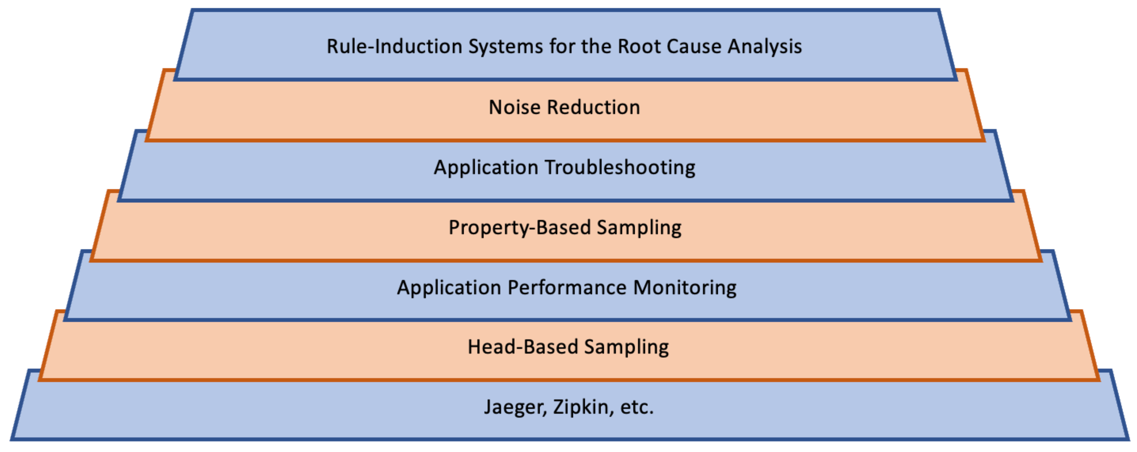
In this paper, we vote for a multi-purpose and hierarchical sampling strategy focusing on the efficiency of application troubleshooting and root cause analysis. We are considering a multi-layered approach to efficiently capture and preserve different types of information within a system (see
Figure 1). The first layer enables distributed tracing to track requests or transactions through the application we monitor. The second layer initiates head-based (rate-based) sampling for a general volume reduction. The goal is to obtain a manageable amount of data for further analysis in "Application Performance Monitoring" while retaining a representative sample of the overall system behavior.
The next layer, "Property-Based Sampling," retains information by incorporating sampling, which preserves useful properties like trace type, latency, errors, etc. Trace-type sampling involves categorizing traces based on their characteristics or origins within the system. Latency-based sampling, on the other hand, prioritizes the collection of traces associated with significant delays or performance bottlenecks. Error-based sampling identifies and retains traces associated with errors, exceptions, or other abnormal conditions within the application. Combining those approaches allows the system to store more diverse traces, ensuring that valuable information across different categories and performance metrics is captured. By isolating and storing those traces, developers and system administrators have the necessary data to diagnose and address issues effectively, improving overall system reliability and performance. The "Application Troubleshooting" layer monitors performance degradations by tracing traffic passing through different microservices. The visualization of the tracing traffic is known as the Application Map. It helps visualize malfunctioning services. The detection can be performed by increasing the percentage of erroneous traces or typical latencies. The issues will be analyzed by tracing traffic passing through that specific degraded microservice. The next layer performs noise reduction by rate-based sampling focusing on erroneous traces. It preserves all dominant normal and erroneous traces and removes the rare ones. This approach is acceptable when the problem has already been detected, and the goal is to explain it. The final layer applies rule learning systems to the tracing traffic, revealing recommendations connected to trace errors. The system administrators can inspect the recommendations to accelerate remediation.
Overall, this hierarchical sampling approach efficiently manages trace data by prioritizing information based on its relevance and importance for system analysis and troubleshooting. It balances the need to reduce data volume with the requirement to retain critical details for comprehensive understanding and problem resolution.
One of the main benefits of distributed tracing is improved application performance, resulting in reduced mean time to detect (MTTD) and mean time to repair (MTTR) IT issues. Distributed tracing enables penetration to the bottom of application performance issues faster, often before users notice anything wrong. Upon discovering an issue, tracing can rapidly identify the root cause and address it. It also provides early warning capabilities when microservices are in poor health and highlights performance bottlenecks anywhere. However, this task is only feasible for a few system administrators or site reliability engineers (SREs) due to the large scale of modern distributed environments. The solution is an AI for IT Operations (AIOps) strategy that leverages AI-powered software intelligence to automate developments, service deliveries, and troubleshooting. AIOps is a real game-changer for managing complex IT systems.
In AIOps, where machine learning algorithms analyze vast amounts of data to automate IT operations and decision-making processes, transparency and interpretability are paramount. Trust in AIOps hinges on implementing Explainable AI (XAI) solutions (see [
19]). Those techniques enable stakeholders to understand and interpret the decisions made by AI models, build confidence in their reliability, and facilitate human-AI collaboration. By providing insights into how AI algorithms arrive at their conclusions, XAI fosters trust among users, reduces the risk of biased or erroneous outcomes, and enhances the adoption and effectiveness of AIOps solutions. We focus on rule-learning systems and show their efficiency in combination with trace sampling. Rule induction systems, such as RIPPER (Repeated Incremental Pruning to Produce Error Reduction) (see [
20]) and C5.0 rules (see [
21]), are common examples of XAI solutions.
Figure 2 shows the transformation of erroneous traces into insights based on rule-induction systems. First, we construct features based on traces and their spans. The volume of traces after the sampling will be adequate to carry out that generation procedure. For some systems, the number of features can be rather large. Second, rule-learning methods solve the corresponding classification problem and generate rules that can explain/predict the nature of the group of traces that arrive as erroneous. These learning systems generate understandable rules based on input data. Humans can easily comprehend those rules, which provide clear insights into the decision-making process of the AI model. Unlike black-box machine learning models such as deep neural networks, where it’s often challenging to understand how the model arrives at its predictions, rule induction systems offer transparency. Users can inspect the rules to understand the underlying logic and reasoning behind the rules. This enhances the trustworthiness of the AI system.
This analysis reveals the underlying causes of the errors and potential areas for improvement or mitigation. By interpreting the induced rules, developers and system administrators can gain insights regarding the possible remediation of issues. The rules provide transparent and interpretable explanations of certain errors occurring under specific conditions or scenarios. Armed with insights from the root cause analysis, appropriate measures can be taken to optimize the system, fix bugs, or implement preventive measures to reduce the likelihood of similar errors occurring in the future.
Understanding how error-based sampling in the final stage affects the rules and simplifies the recommendations is one of our goals. It preserves dominant errors while potentially removing rare events across different types. Error-based sampling focuses on data points with higher errors or uncertainties. Certain errors in many datasets may occur more frequently or significantly impact the overall analysis. Rare events in a dataset often contribute to its overall uncertainty, especially if they are outliers or anomalies. These events may skew statistical measures or model predictions, making it challenging to draw reliable conclusions. Error-based sampling may downplay the influence of rare events by sampling them less frequently or excluding them altogether. We show how this reduction in outliers helps to stabilize the analyses and make recommendations more robust to extreme cases.
The paper is organized as follows.
Section 2 describes the main trends of trace sampling and rule-induction.
Section 3 explains the methods of trace sampling based on properties when the goal is to preserve all available types, latencies, and errors uniformly.
Section 4 presents the impact of noise reduction on a rule induction when the goal is to preserve only frequent erroneous traces across all types.
2. Related Work
Various companies and researchers are developing end-to-end distributed tracing technologies in which sampling is one of the core components as the prevailing approach to reducing tracing overheads. Instead of tracing every request, the sampling only captures and persists traces for a subset of requests to the system. To ensure the captured data is useful, sampling decisions are coherent per request – a trace is either sampled in its entirety, capturing the full end-to-end execution, or not at all. Sampling effectively reduces computational overheads; these overheads are only paid if a trace is sampled, so they can be easily reduced by reducing the sampling probability (see [
22,
23,
24,
25] with references therein).
Large technology companies such as Google, Microsoft, Amazon, and Facebook often develop methods to monitor and analyze the performance of their own systems and applications. Early tracing systems such as Google’s Dapper (see [
26]) and later Facebook’s Canopy (see [
27]) make sampling decisions immediately when a request enters the system. This approach, known as head-based sampling, avoids the runtime costs of generating trace data as it occurs uniformly at random, and the resulting data is simply a random subset of requests. In practice, sampling rates can be as low as
(see [
22]).
Tail-based sampling is an alternative to head-based sampling. It captures traces for all requests and only decides whether to keep a trace after it has been generated. While OpenTelemetry (see [
28]) offers a tail-based sampling collector, its implementation presents challenges as storing all spans of a trace until the request concludes demands a sophisticated data architecture and solutions. One such end-to-end tracing to enhance distributed system dependability by dynamically verifying and diagnosing correctness and performance issues is proposed in paper [
29]. The idea is based on clustering execution graphs to bias sampling towards diverse and representative traces, even when anomalies are rare.
Google has developed distributed tracing technologies, such as Google Cloud Trace and OpenCensus, which allow users to collect and analyze trace data from applications running on Google Cloud Platform and other environments. Each Google Cloud service makes its own sampling decisions. When sampling is supported, that service typically implements a default sample rate or a mechanism to use the parent’s sampling decision as a hint as to whether to sample the span or maximum sampling rate (see [
30]). OpenCensus provides "Always," "Never," "Probabilistic," and "RateLimiting" samplers. The last one tries to sample with a rate per time window, which by default is 0.1 traces/second (see [
31]).
Azure Application Insights sampling (see [
32]) aims to reduce telemetry traffic, data, and storage costs while preserving a statistically correct analysis of application data. It enables three different types of sampling: adaptive sampling, fixed-rate sampling, and ingestion sampling. Adaptive filtering automatically adjusts the sampling to stay within the given rate limit. If the application generates low telemetry, like during debugging or low usage, it doesn’t drop items as long as the volume stays under the limits. The sampling rate is adjusted to hit the target volume as the telemetry volume rises. Fixed-rate sampling reduces the traffic sent from web servers and web browsers. Unlike adaptive sampling, it reduces telemetry at a fixed rate a user decides. Ingestion sampling operates where web servers, browsers, and devices telemetry reaches the Application Insights service endpoint. Although it doesn’t reduce the telemetry traffic sent from an application, it does reduce the amount processed and retained (and charged for) by Application Insights. Microsoft researchers introduced an observability-preserving trace sampling method, denoted as STEAM, based on Graph Neural Networks, which aims to retain as much information as possible in the sampled traces (see [
33]).
In 2023, AWS announced the general availability of the tail sampling processor and the group-by-trace processor in the AWS Distro for OpenTelemetry collector (see [
34]). Advanced sampling refers to the strategy where the Group By Trace processor and Tail Sampling processor operate together to make sampling decisions based on set policies regarding trace spans. The Group By Trace processor gathers all of the spans of a trace and waits a pre-defined time before moving them to the next processor. This component is usually used before the tail sampling processor to guarantee that all the spans belonging to the same trace are processed together. Then, the Tail Sampling processor samples traces based on user-defined policies.
There are also many other companies developing such technologies. We will mention a few of them. Jaeger is an open-source distributed tracing system developed by Uber Technologies. It is widely used for monitoring and troubleshooting microservices-based applications (see [
35]). Zipkin is another open-source distributed tracing system originally developed by Twitter. It helps developers gather data for various components of their applications and troubleshoot latency issues (see [
36]). LightStep is a commercial company that offers tracing solutions for monitoring and troubleshooting distributed systems (see [
37]). Datadog is a monitoring and analytics platform that offers features for collecting and analyzing traces, logs, and metrics from applications and infrastructure (see [
38]). Dynatrace is a software intelligence platform that provides features for monitoring and analyzing the performance of applications and infrastructure, including distributed tracing capabilities (see [
39]). New Relic offers a monitoring and observability platform that includes features for collecting and analyzing traces, logs, and metrics from applications and infrastructure (see [
40]). AppDynamics is an application performance monitoring solution that provides features for monitoring and troubleshooting applications, including distributed tracing capabilities (see [
41]). Honeycomb is an observability platform that offers features for collecting and analyzing high-cardinality data, including traces, to debug and optimize applications (see [
42]). Grafana is an open-source analytics and visualization platform that can visualize traces, logs, and metrics collected from various sources, including distributed tracing systems (see [
43]). Elastic is the company behind Elasticsearch, Kibana, and other products in the Elastic Stack. Their solutions offer features for collecting, analyzing, and visualizing traces, logs, and metrics (see [
44]).
System administrators can no longer perform real-time decision-making due to the growth of large-scale distributed cloud environments with complicated, invisible underlying processes. Those systems require more advanced and ML/AI-empowered intelligent RCA with explainable and actionable recommendations (see [
45,
46,
47,
48,
49,
50,
51,
52,
53] with references therein).
XAI (see [
19]) builds user and AI trust, increases solutions’ satisfaction, and leads to more actionable and robust prediction and root cause analysis models. Many users think it is risky to blindly trust and follow AI recommendations and predictions, and they need to understand the foundation of those insights. Many ML approaches, like decision trees and rule-induction systems, have sufficient explainability capabilities for RCA. They can detect and predict performance degradations and identify the most critical features (processes) potentially responsible for the malfunctioning.
In many applications, explainable outcomes can be more valuable than conclusions based on more powerful approaches that act like black boxes. Rule learners are the best if outcomes’ simplicity and human interpretability are superior to the predictive power The list of known rule learners consists of many exciting approaches. We refer to [
54] for a more detailed description of available algorithms, their comparisons, and historical analysis. It contains relatively rich references and describes several applications (see also [
20,
21,
55,
56,
57,
58]). Rule learning algorithms have a long history in industrial applications (see [
7,
14,
59,
60,
61,
62,
63,
64,
65,
66]). Many such applications utilize classical classifiers like C5.0Rules (see [
21]) and JRip. The last one is the Weka implementation of RIPPER.
The recommendations derived from rule-learning systems can be additionally verified regarding uncertainty based on Dempster-Shafer’s theory (DST) of evidence [
67]. It is an inference framework with uncertainty modeling, where independent sources of knowledge (expert opinions) can be combined for reasoning or decision-making. In [
68], it is leveraged to build a classification method that enables a user-defined rule validation mechanism. These rules are "encoding" expert hypotheses as conditions on the data set features that might be associated with certain classes while making predictions for observations. It provides a “what-if” analysis framework for comprehending the underlying application, as it is applied in [
69]. This means that in the current study context, we can apply the same framework to estimate the effectiveness of the trace sampling approaches while comparing the rule validation results in the pre- and post-sampling stages. DST is overlooked in terms of learning algorithms that could be utilized in predictive system diagnostics (see the survey [
45], which emphasizes that gap). Therefore, its application in our use case of RCA-effective trace sampling is an additional novelty we introduce.
3. Trace Sampling Based on Type, Duration, and Errors
Modern distributed applications trigger an enormous number of traces. Direct storage of hundreds of thousands of traces heavily impacts users’ budgets. A sampling strategy is a procedure that decides which traces to store for further utilization. We describe a procedure that samples traces based on their types, durations, and/or errors. The final goal is to preserve sufficient information for application troubleshooting without possible distortion.
A trace type can be approximately identified by the root span or the span that arrived at the earliest. More strict identification is based on the analysis of its structure. However, the latest is rather resourceful and will require additional grouping/clustering approaches. The durations of traces (in milliseconds) are available in the corresponding metadata. It is possible to extract the durations for different trace types and estimate the average/typical durations of the corresponding processes. The information on errors is also available in trace metadata. Traces are composed of spans. We have detailed information regarding the spans in the corresponding tags that describe the micro-processes. One of the tags indicates the health of a span. We can assume that the entire trace is erroneous if at least one of its spans has a "True" error label. We suggest a parametric approach for all sampling scenarios, allowing us to modify the required percentage of compression rates accordingly.
3.1. Sampling by a Trace Type
Assume that we know how to determine a trace type. Let
M be the number of trace types for a specific period and
be the number of traces in each type. This information should be collected/updated for a recent period as the number of trace types and the trace-flow velocity are subject to rapid changes in modern applications. Let
N be the number of all traces before the sampling:
and
be the probability of the occurrence of the
k-th type. Let
and
,
be the sampling rate (the percentage/fraction of stored traces) and the number of traces after the sampling of the
k-th type, respectively:
where
should be rounded to the closest integer. Also, we denote by
the total number of all traces after the sampling
The ratio
is the final sampling rate. We propose to compute the sampling rate
as inversely proportional to the probability
:
where
is a parameter a user should determine to satisfy the needed final sampling rate
r. Generally, the more frequent a trace type, the lower the corresponding sampling rate
.
Let us see how the parameter
should be determined if the final user requirement is known:
where
It can be considered an analog of the Gini index showing the total sampling rate. For a specific dataset of traces, we can compute the values of
across different
and determine its value to satisfy a user’s requirement. We can try to estimate the proper value of
based on the recent collection of traces (say for the recent 2 hours) and dynamically update those values to meet the requirement.
Let us illustrate how this procedure works for a specific application.
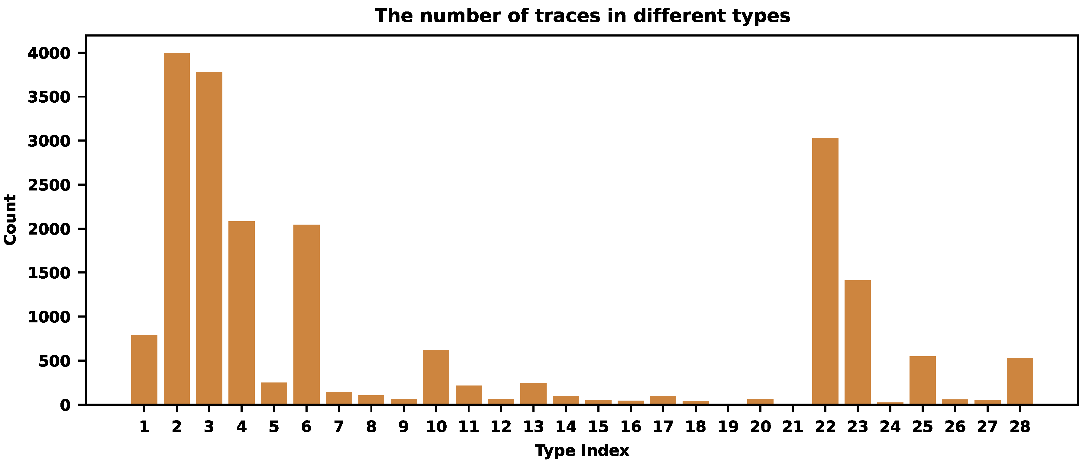
Figure 3 shows the distribution of traces across different trace types.
There are types with almost 4000 traces and very rare ones, like with 3 representatives. Overall, we detected 20425 traces distributed across 28 different trace types.
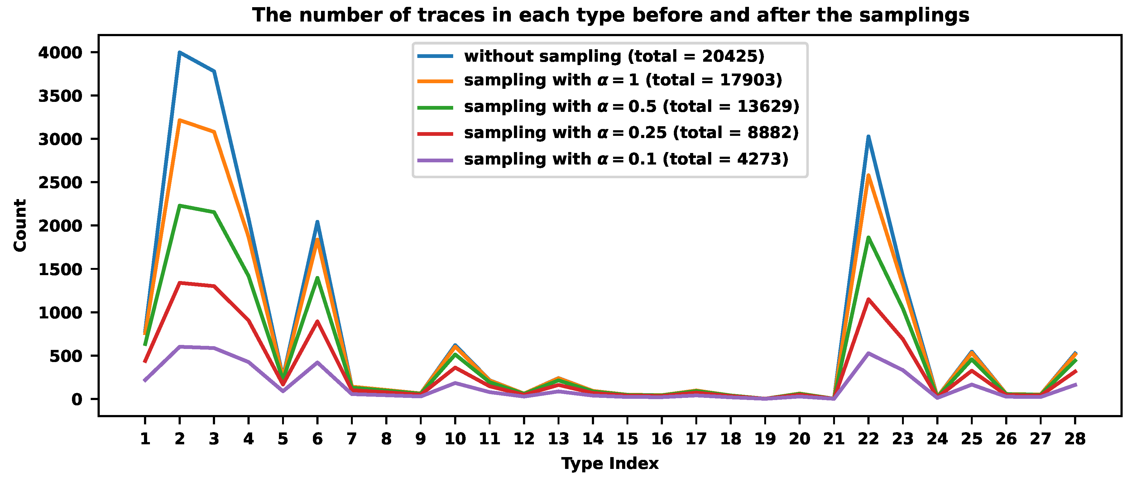
Figure 4 and
Table 1 reveal how different rates compress traces across types. We experimented with
and
. The sampling rate is always smaller for common trace types and larger for rare ones (see
Table 1). Smaller values of
correspond to smaller final sampling rates. When
, we store 17903 traces across all types,
of all traces. When
, we store 13629 traces,
of all traces. For
, we store 8882 traces,
. When
, we store 4273 traces,
of all traces.
Let us inspect some of the sampling rates for specific types. The most frequent type contains 3996 traces with the probability . The corresponding sampling rate (for ) is , and 3215 traces from this class were stored. One of the rarest types contains 3 traces with almost zero probability. The sampling rate is almost , and we store two or three traces for different .
The correct value of
that will satisfy a user requirement could be estimated by computing the
values.
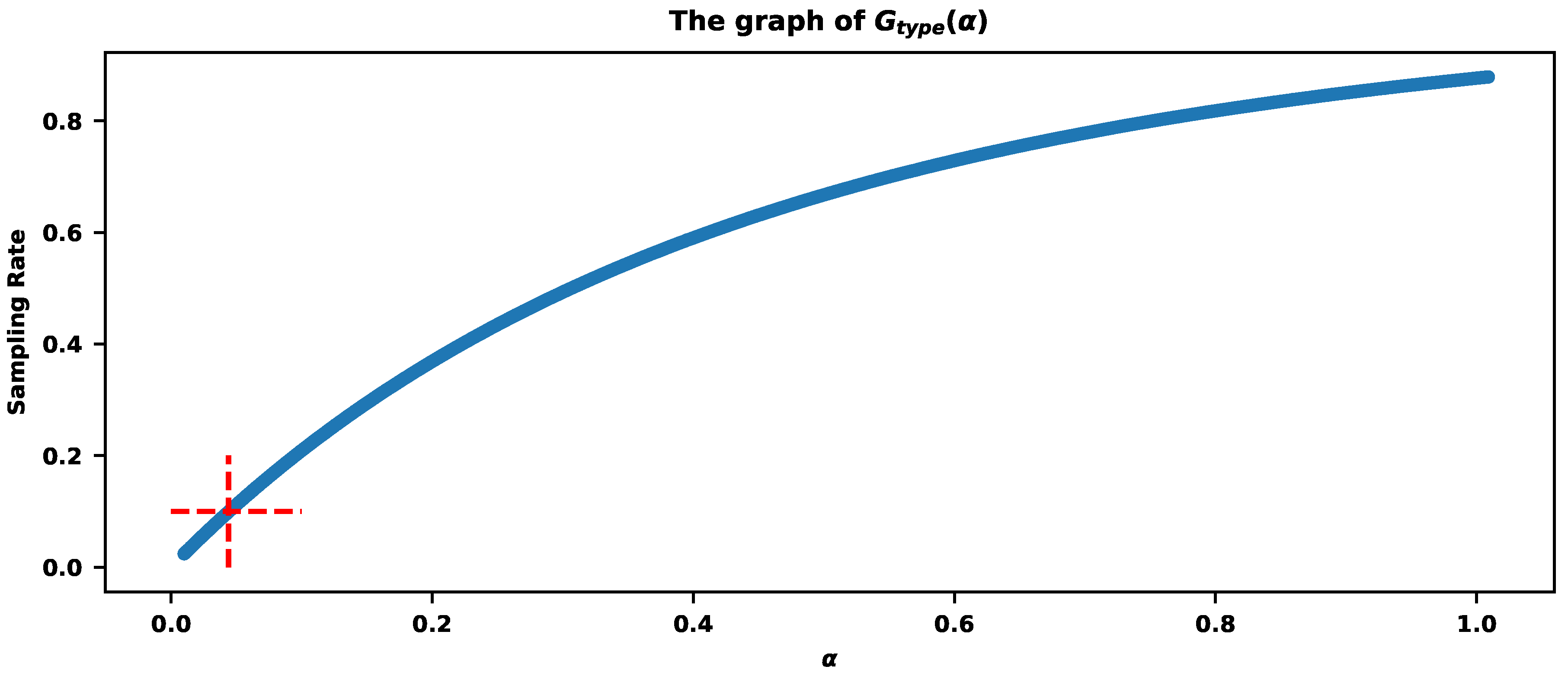
Figure 5 explains the procedure. Let us assume that the required sampling rate is
, meaning we want to store around that percentage of traces.
provides a sampling rate
.
This algorithm should be applied if trace types carry important information on an application, and both rare and frequent types should be preserved for further analysis. Mathematically, it means no more than, say, 50 trace types with diverse frequencies. Diversity can be inspected via the Gini index or entropy. If those measures are close to zero, the sampling will try to maximize them and store equal portions from all types.
3.2. Sampling by a Trace Duration
In this subsection, we consider the sampling of traces based on their durations. This setup is reasonable if we have a few trace types where traces have almost the same average durations. We would like to keep all traces with some average durations and those with extraordinary short or long ones.
Assume
N traces with durations
. Let
be the corresponding histogram of durations with
m number of bins:
where
,
be the number of traces with durations within intervals
,
and
with durations within
. Let
,
be the probability that a trace has a duration from the
s-th bin:
We determine the sampling rate
of a trace with duration within the
s-th bin to be inversely proportional to the corresponding probability
:
where
is the parameter to meet a user’s requirement.
Let
be the number of traces after the sampling in the
s-th bin:
Let
be the total number of traces after the sampling:
where
is the total sampling rate for different values of parameter
.
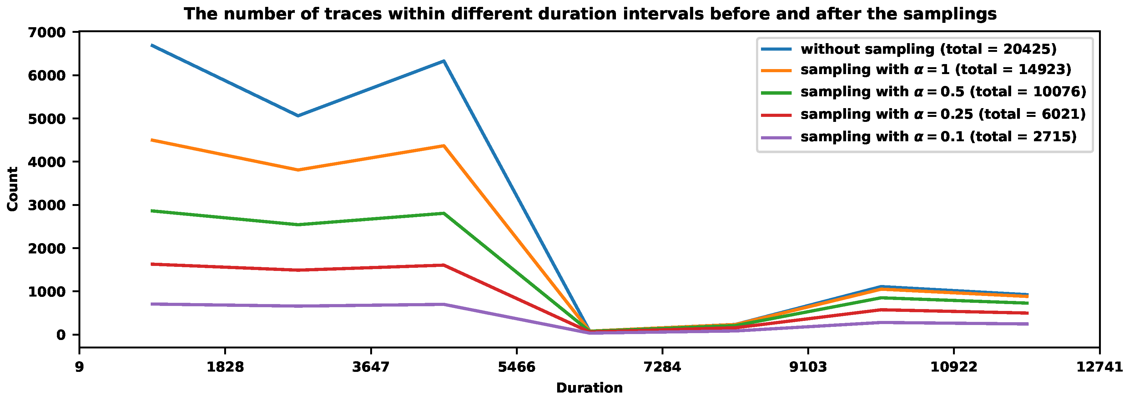
Let us illustrate how this procedure works for the same dataset of traces presented earlier. We will skip the trace types and will look into the trace durations.
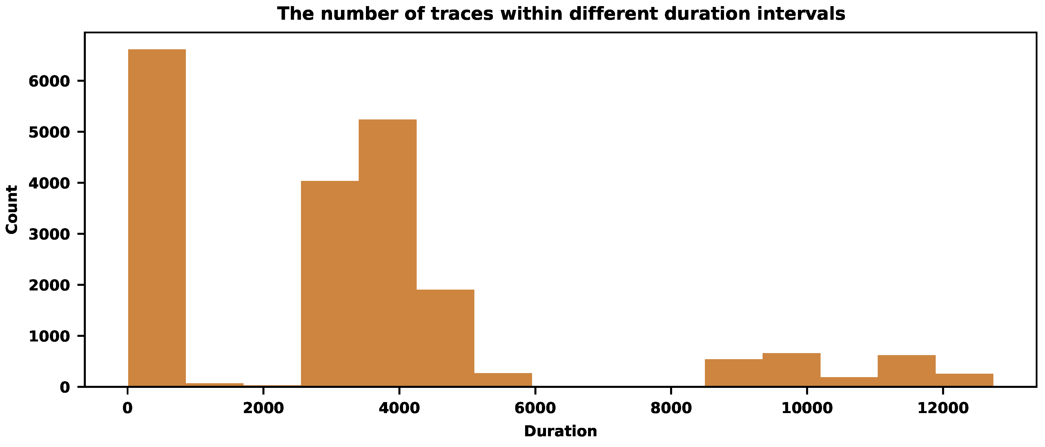
Figure 6 shows the distribution of traces with durations in different time intervals. It shows three dominant time intervals where the most traces are concentrated. We can aggressively sample those frequent traces and moderately sample the rare ones outside dense areas.
Table 2 shows how the sampling procedure works for different
parameter values (we use 7 bins).
The first column, "Time intervals" of
Table 2, shows the seven intervals of durations. The intervals have equal lengths, although the bins could be nonuniform. The second column shows the initial number of traces with the durations within the corresponding time intervals. The remaining columns show the numbers after the sampling with the corresponding
. The last row of
Table 2 reveals the final sampling rates. The bigger the value of
, the more severe the reduction of traces. The value
provides a sampling rate of around
.
Figure 7 visualizes the results of
Table 2.
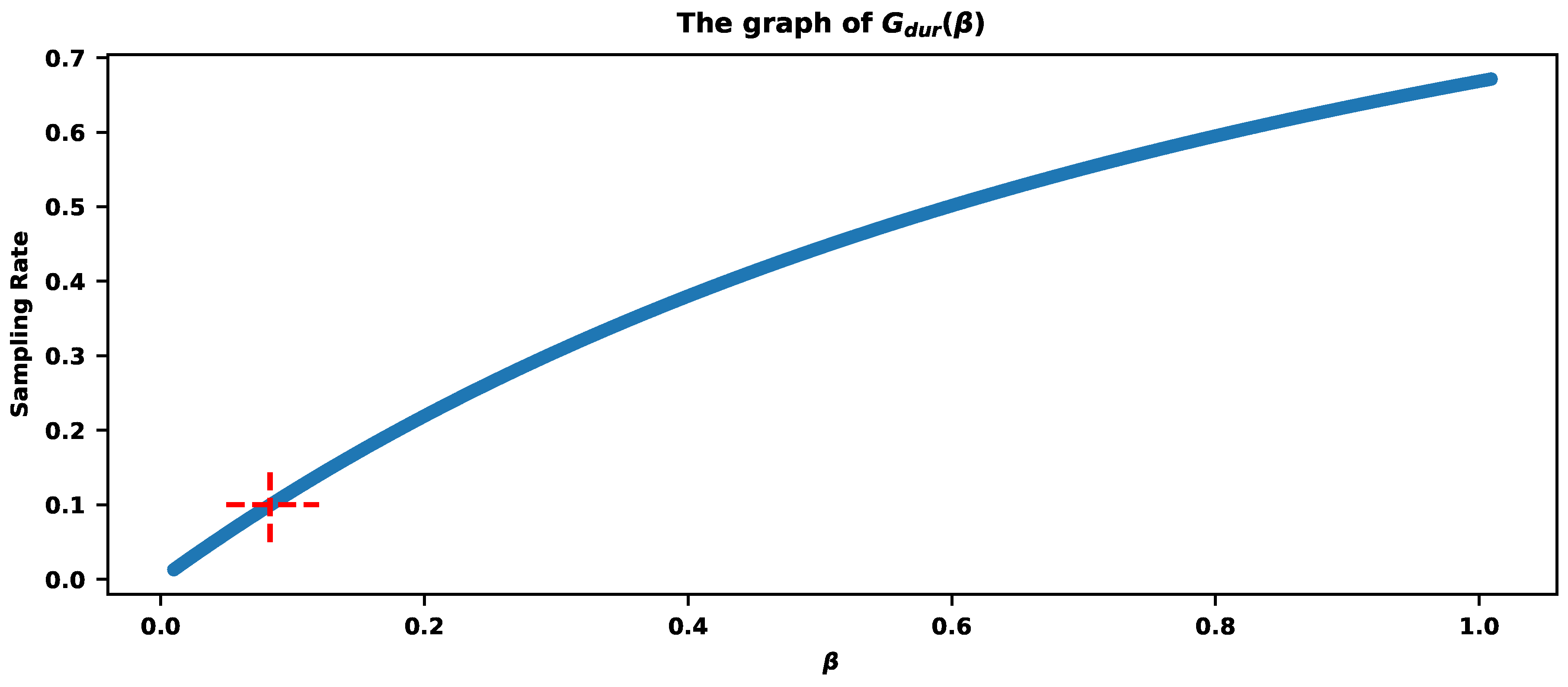
If the requirement is to sample exactly
of traces, then
Figure 8 shows the parameter
estimation based on the values of
. The red cross indicates that
provides the sampling rate
.
Proper histogram construction is a crucial milestone for frequency-based sampling. In general, the problem is the impact of outliers on the bin construction process. Standard procedures use an equidistant split of the data range, and data outliers can enlarge it, resulting in big bins with resolution distortion. The more accurate procedure should involve outlier detection to preserve them in separate bins with further application of the classical procedure for the main part of the data. We consider outlier detection via a modified MAD (median absolute deviation) algorithm (see [
70]) with a slight modification. We define upper and lower baselines as
and
quantiles of data:
where
is the
s-th quantile of data with
. We calculate the upper and lower distances:
where
are data points bigger than or equal
and
are data points smaller or equal than
. We set upper and lower MADs as
Based on the MADs, upper and lower thresholds are defined as:
and
All data points lying upper or lower than the corresponding thresholds are assumed to be upper and lower outliers, respectively. We cut outliers from the data and construct the classical histogram for the remaining data with some predefined number of bins (say bins = 5). Then, we calculate the number of lower and upper outliers and append them to the main histogram from left and right, respectively.
Hence, if data have small-value outliers, then the first bin of the histogram contains the number of data points within the interval . If data have big-value outliers, the last bin contains the number of data points within the interval . The main part of the histogram relates to data points within the interval . This procedure allows proper construction of the corresponding histograms with a small number of bins. It is worth noting that the main part of the histogram consists of uniform intervals, while the widths of the first and last bins could be different from those bins. Finally, if data have outliers from both sides, the corresponding histogram has final bins. If data have outliers only from one side, then the final number of bins is . No other bins are added to the classical histogram if data come without outliers.
3.3. Hybrid Approach Based on Types and Durations
The hybrid approach takes into account both trace type and duration information. This algorithm performs accurate sampling if both durations and types are important. Assume that traces are already grouped into trace types. We generate the histogram of durations for each group and apply the procedure described in the previous subsection. We also consider the probability of a trace type. Common types will be sampled more aggressively.
Let
be the histogram of durations of the
k-th trace type and
be the number of traces in the
s-th bin of the
k-th type. As above,
M is the number of different types, and
m is the number of bins in the histogram. Let
be the number of traces in the
k-th trace type:
Let
N be the total number of traces:
Let
and
We denote the sampling rate of a trace from the
s-th bin of the
k-th trace type by
. It shows the fraction of traces that should be stored. We compute it by the following formula as inversely proportional to the corresponding probabilities:
where
are some unknown parameters to be tuned to meet the requirement for the final sampling rate
r.
Let us show how it could be done. Let
be the number of traces in the
k-th trace type after the sampling. Let
be the number of traces in the
s-th bin and the
k-th trace type after the sampling:
Let
be the total number of traces after the sampling across all types and durations:
where
is the required final sampling rate that can be accomplished by appropriately selecting parameters
and
.
First, we will illustrate this procedure when
.
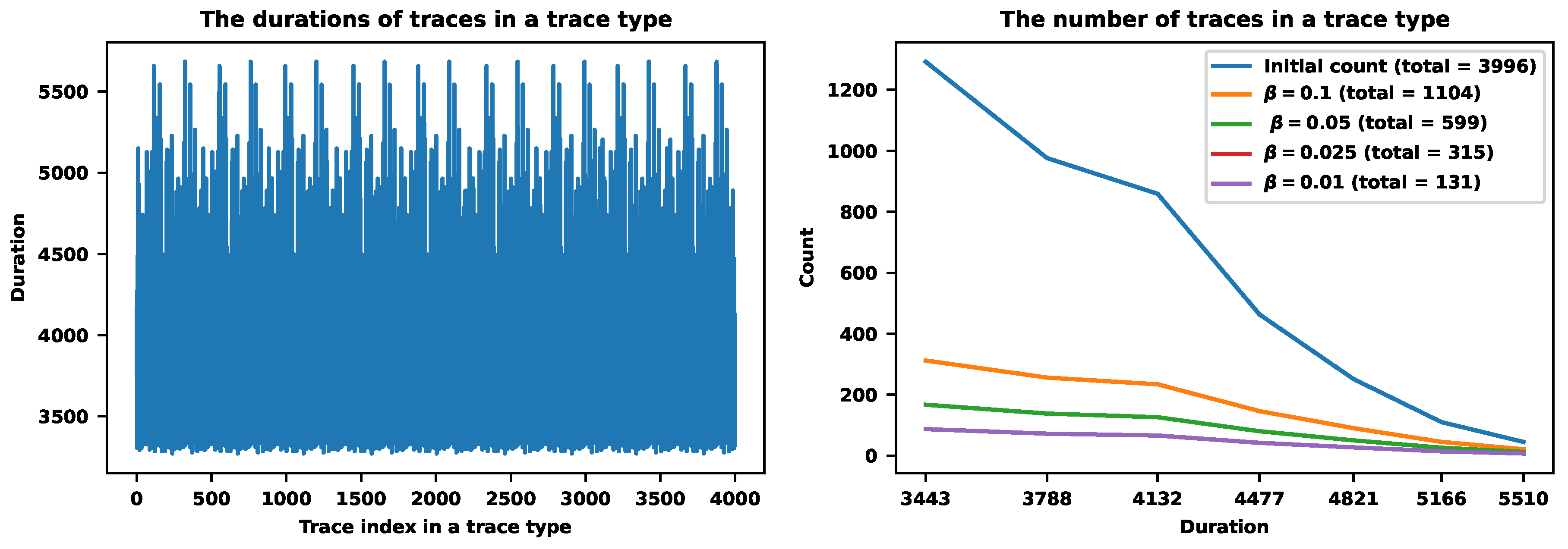
Figure 9 reveals the procedure for a specific trace type containing 3996 traces. The left figure shows the scatter plot of durations. The right figure shows the histogram of durations with 7 bins before and after the samplings. The value
corresponds to the sampling that stores 1104 traces. The next value
stores 599 traces. The value
corresponds to the sampling with 315 preserved traces. Finally, the value
stores 131 traces. The last one corresponds to the
sampling rate. By the way, the probability of this trace type is
, which also impacts the sampling rates with
setting.
Figure 9.
The hybrid approach for a specific trace type (N2 in
Figure 11). The left figure shows the plot of durations. The right figure shows the counts of traces in different bins before and after the samplings corresponding to different values of
.
Figure 9.
The hybrid approach for a specific trace type (N2 in
Figure 11). The left figure shows the plot of durations. The right figure shows the counts of traces in different bins before and after the samplings corresponding to different values of
.
Figure 10.
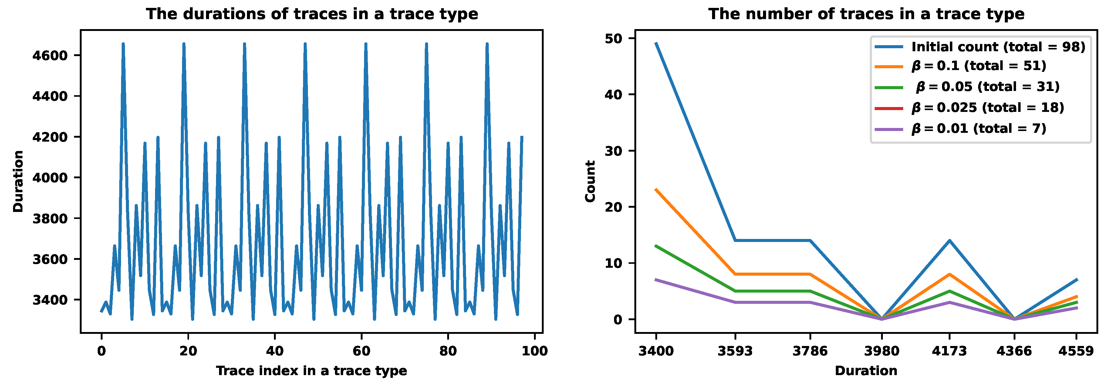
The hybrid approach for a specific trace type (N17 in
Figure 11). The left figure shows the plot of durations. The right figure shows the counts of traces for
.
Figure 10.
The hybrid approach for a specific trace type (N17 in
Figure 11). The left figure shows the plot of durations. The right figure shows the counts of traces for
.
Figure 11.
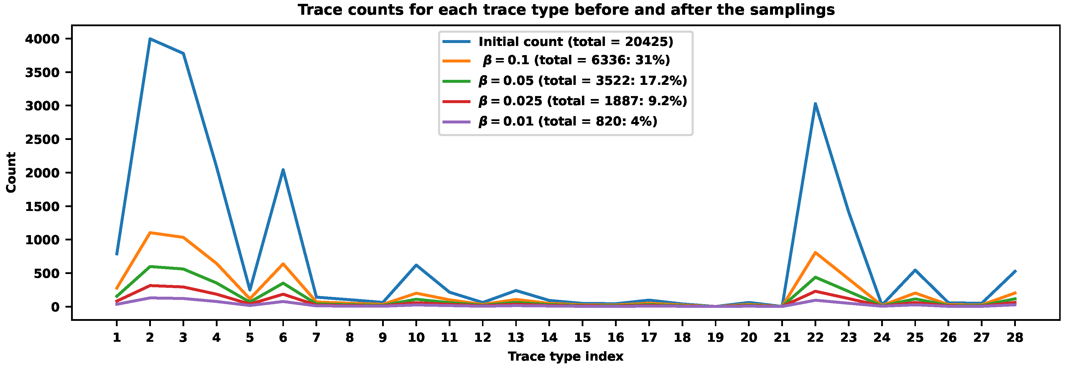
The hybrid sampling approach for .
Figure 11.
The hybrid sampling approach for .
Figure 10 shows the hybrid procedure for another trace type with the probability
. It contains only 98 traces and is a rare type compared to the previous example. It also corresponds to the setting
. The right figure shows the sampling results for different values of
. For example, the value
corresponds to the sampling that stores only 7 traces of this specific type. It corresponds to the
sampling rate. The value
corresponds to the
sampling rate. The value
stores 31 traces and corresponds to the
sampling rate. Finally, the value
corresponds to the sampling rate
.
Figure 11 shows the result of the hybrid approach across different trace types when
. The total sampling rate is
for
. The values
correspond to the sampling rate
. It means that the values of
and
can control the sampling rates in a wide range of values. If we need to accomplish a strict requirement, we can turn to the
values corresponding to the sampling rates.
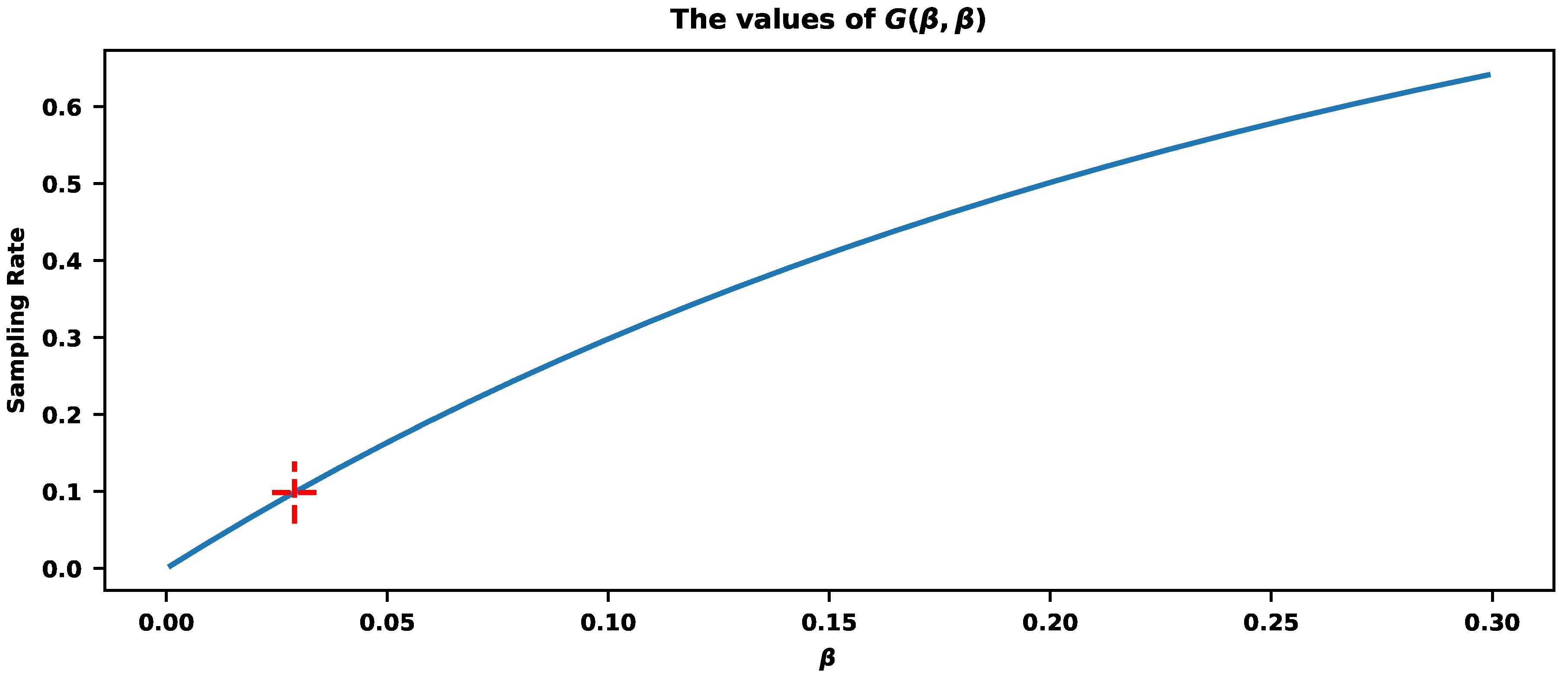
Figure 12 shows the values of
, where the red cross corresponds to the sampling rate of
(the exact value of
G is
) with
. We can also tune the values of
and
independently.
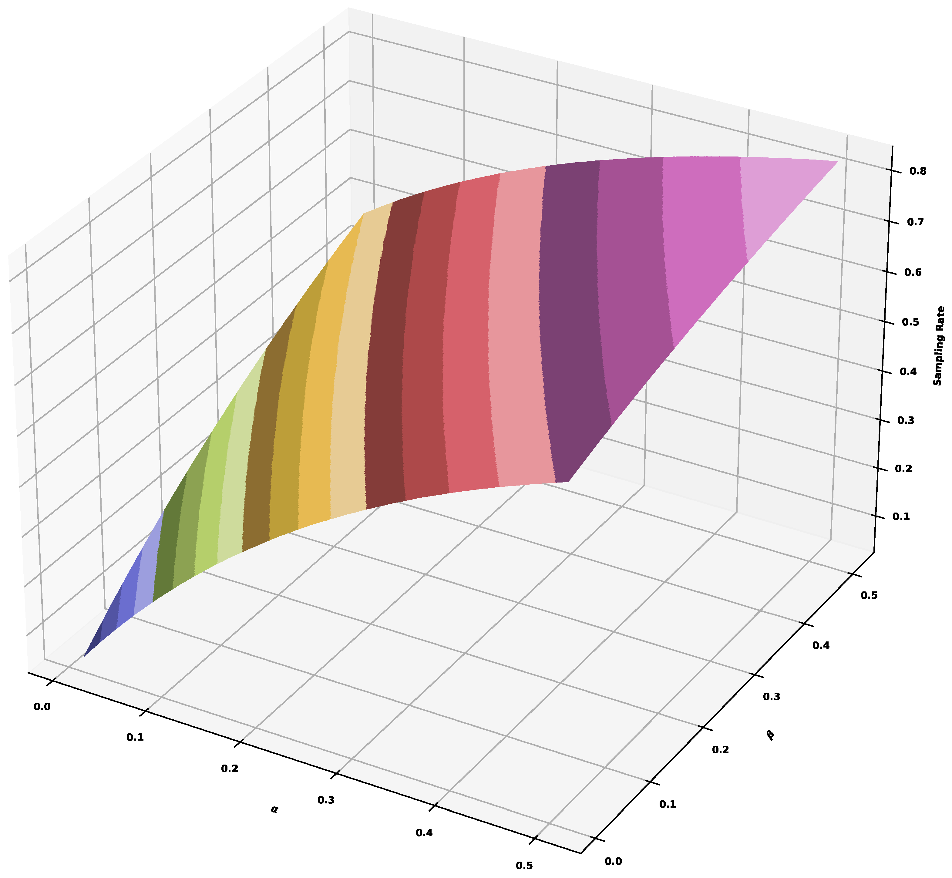
Figure 13 shows the surface of sampling rates corresponding to different values. For example, the total sampling rate of
can be accomplished by
, or
, or
, or
, or
, etc.
Parameter optimization can be performed without the utilization of long historical data. We can take an initially random value for the parameters and, after each hour, verify the actual compression ratio. Then, by increasing or decreasing the values, we achieve the required sampling. This will work especially for dynamic applications when relying on available historical information is impossible.
How, in practice, can we sample a trace? When a specified trace (with known type and duration) is detected with a known sampling rate r, a random variable from distribution should be generated. This random variable has a boolean outcome with the value 1 that has probability r and value 0 with the probability . If the outcome is 1, we store the specified trace; otherwise, we ignore it. This will allow us to store the traces with the required sampling rates in the long run.
Returning to the problem of histogram construction, we refer to a powerful approach known as the t-digest algorithm (see[
71]), which addresses several problems in histogram construction. The first concern corresponds to storing time series data with trace durations. For each trace type, we need to store the corresponding time series of durations for further histogram construction, and we need those time series with sufficient statistics. For 28 trace types, as in our experiments, we need to store the 28 time series. The second concern corresponds to the process of histogram construction. Each time when we need those histograms, sorting should be applied to the corresponding data of durations, and the procedure must be repeated each time in case of some new arrivals. The concern is the impact of outliers. An efficient solution to the mentioned problems is the t-digest algorithm. Instead of storing the entire time series data, it stores only the result of data cluster centroids and data counts in each cluster. The efficient merging approach allows for combining different t-digest histograms, making the entire process streaming. The t-digest is very precise while estimating extreme data quantiles (close to 0 and 1), making the procedure robust to outliers.
3.4. The Sampling of Erroneous Traces
In specific frameworks, sampling should preserve other important properties besides durations and types. One such property is the normality/abnormality of a trace, which characterizes microservices performance and could be used for troubleshooting and root-cause analysis. In the described approach, we can’t guarantee a sufficient number of important erroneous traces in the sampled dataset, as there was no requirement to preserve them. Now, we will try to address that requirement by discussing various approaches.
The first approach is the natural modification of the previous one, assuring the existence of enough erroneous traces in each trace type after the sampling. More precisely, we verify the existence of erroneous traces in each trace type. If they exist, we divide the corresponding type into two types containing only normal or erroneous traces. Then, we can apply the approach that has already been considered (sampling by type, duration, or hybrid) to the same dataset but with renewed trace types.
Dividing erroneous traces into additional types by the corresponding error codes is also possible. Assume that trace type "A" has erroneous traces containing error codes "400-Bad Request" and "401-unauthorized". Then, we can divide it into three new trace types "A-we" (without errors), "A-400" (with 400 code), and "A-401" (with 401 code). It is also possible to divide erroneous traces into types by their error codes independently of the types. Say, collect all traces with "400" error codes together in a single type, independently of their original types. Let us show how this approach works.
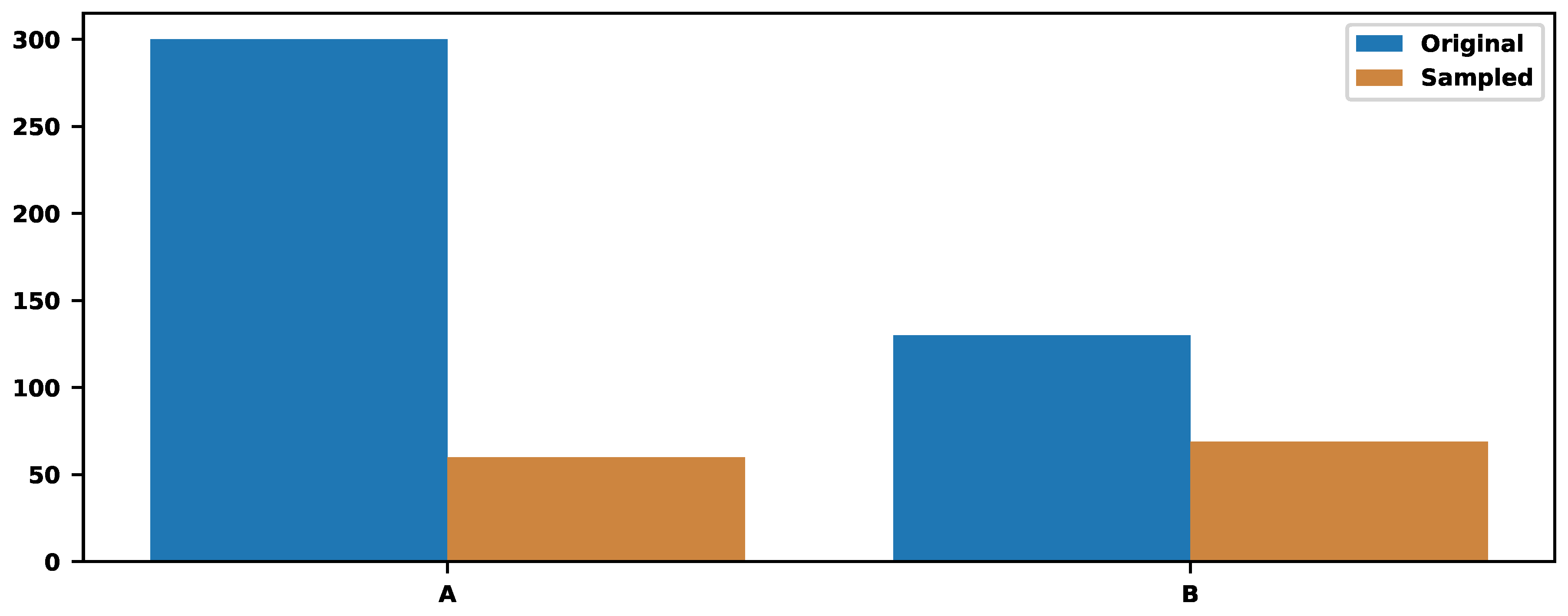
Assume two trace types: 300 traces of type "A" and 130 of type "B," and we must store only
of the traces. The sampling, based only on the trace types, provides the value
. It means storing 60 traces of type "A" and 69 of type "B".
Figure 14 illustrate those numbers.
Now, let us also consider erroneous traces. Assume type "A" has 200 normal and 100 erroneous traces. Thus, types "A" and "A*" contain 200 and 100 traces, respectively. Then, assume type "B" has 60 normal and 70 erroneous traces. Thus, "B" and "B*" contain 60 and 70 traces, respectively. Now, instead of two types, there are four ones. The type-based sampling provides the value , which leads to sampling rates , , , and , respectively.
Figure 15 shows the distributions before and after the samplings. As a result, from 260 normal and 170 erroneous traces, the approach sampled 66 and 63, respectively (see the right figure of
Figure 15). Now, we can guarantee that the final sampled set also contains erroneous traces across different types. It is possible to apply the hybrid approach that will also consider the duration of the erroneous traces.
The second approach tries to control better the percentage of erroneous traces in the sampled dataset. Let
be the final required sampling rate. Assume that
and
are the sampling rates of erroneous and normal traces, respectively:
and
where
and
are the number of normal and erroneous traces before the sampling, respectively, and
and
after the sampling.
Can we also put some requirements on
? We have
and
If the requirements on
h and
lead to the value
, then the requirements can be accomplished. Otherwise, if
turns out to be a negative number, it is impossible, and we must ask to change the requirements.
Let us return to the previous example with two trace types. Can we sample
of traces while preserving
of erroneous ones? We put
and
and try to find appropriate values for
. Our calculations show that
will work. We will preserve the
of erroneous traces and
of normal traces by sampling
of all traces.
Figure 16 illustrates the choices.
4. Troubleshooting of Applications
The ultimate goal of distributed tracing is to monitor application performance, detect malfunctioning microservices, and explain the root causes of problems so that they can be resolved quickly. This is feasible by inspecting the tracing traffic passing through specific microservices, detecting erroneous traces/spans, and trying to explain their origin. Thus, the explainability of ML models is the most crucial property. We consider two highly explainable approaches.
One is RIPPER (see [
20]), which is state-of-the-art in inductive rule learning (see [
55]). It has important technical characteristics, like supporting missing values, numerical and categorical variables, and multiple classes. We experimented with Weka’s RIPPER implementation, or JRip (see [
72]). Application of RIPPER for the inspection of erroneous traces is discussed in [
7]. We are not going into such details but show the impact of noise reduction on the rules.
Next is the Dempster-Shafer classifier considered in [
68]. It is a far more complex approach but has interesting implications. One important characteristic is the ability to measure the uncertainty of specific rules. It should be interesting to compare the uncertainties of the same rules before and after the samplings.
Tracing traffic passing through a malfunctioning microservice can still contain many traces, even after a series of samplings. In this final stage, we apply the sampling of erroneous traces for reducing the volume and simplifying the application of rule induction methods. We aim to understand how the sampling impacts the rule-generation process regarding precision, recall, or uncertainty. It is worth noting that in this stage, the goal of the sampling is not to preserve all possible types and durations of erroneous traces. Exactly the opposite: the goal should be to remove rare erroneous traces and preserve dominant/common ones, as they probably explain the problems of a microservice. This procedure is very straightforward. We separate normal and erroneous traces and additionally separate them by trace types. Then, in all those groups, we sample at the same rate. As a result, some of the groups (rare ones) can vanish. Trace errors or durations can label the resulting dataset (see [
7]). In case of errors, "output=0" corresponds to a normal trace and "output=1" to the erroneous one. We apply RIPPER to explain the origin of erroneous traces.
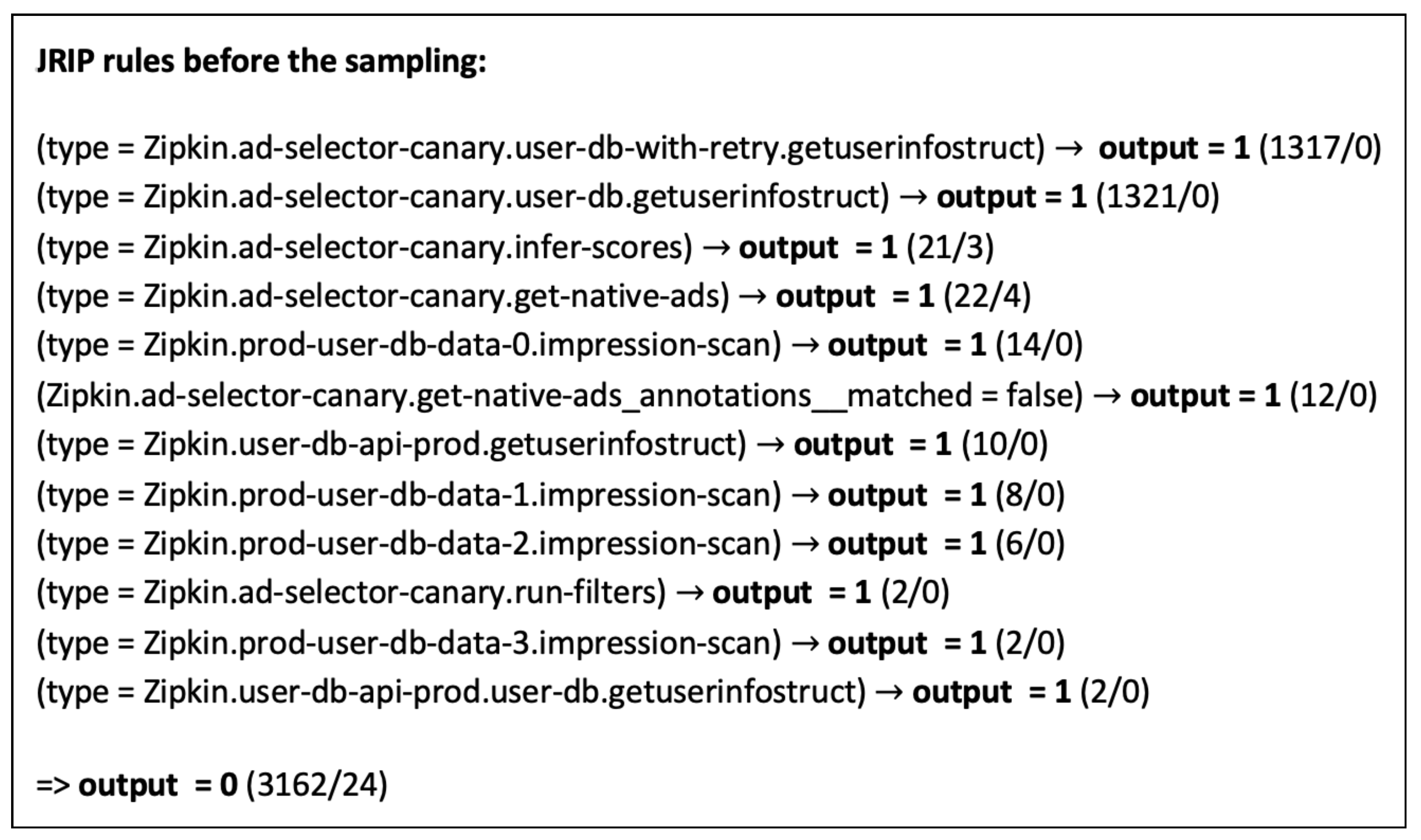
Let us apply this procedure to a real customer cloud environment. The visualization of a tracing traffic is known as an application map. It shows which microservices malfunction and which traces must be collected for troubleshooting. We collected 5899 traces with some 4917 features that should explain the origin of errors. We have 3145 normal and 2754 erroneous traces. JRip (RIPPER) runs for
seconds outputting 13 rules (see
Figure 17).
The first 12 rules describe the erroneous traces. they are mostly connected with the type. Only one of the rules is connected with the tag "-annotations-matched". The fraction at the end of the rule shows how many traces were fired by the rule (numerator) and how many misfired (denominator). The first two rules have large coverage and are precise. The others should be connected with the noise in the dataset. We hope that the sampling will remove the noise. However, the accuracy of this classifier is . The precision and recall of both classes are also bigger than .
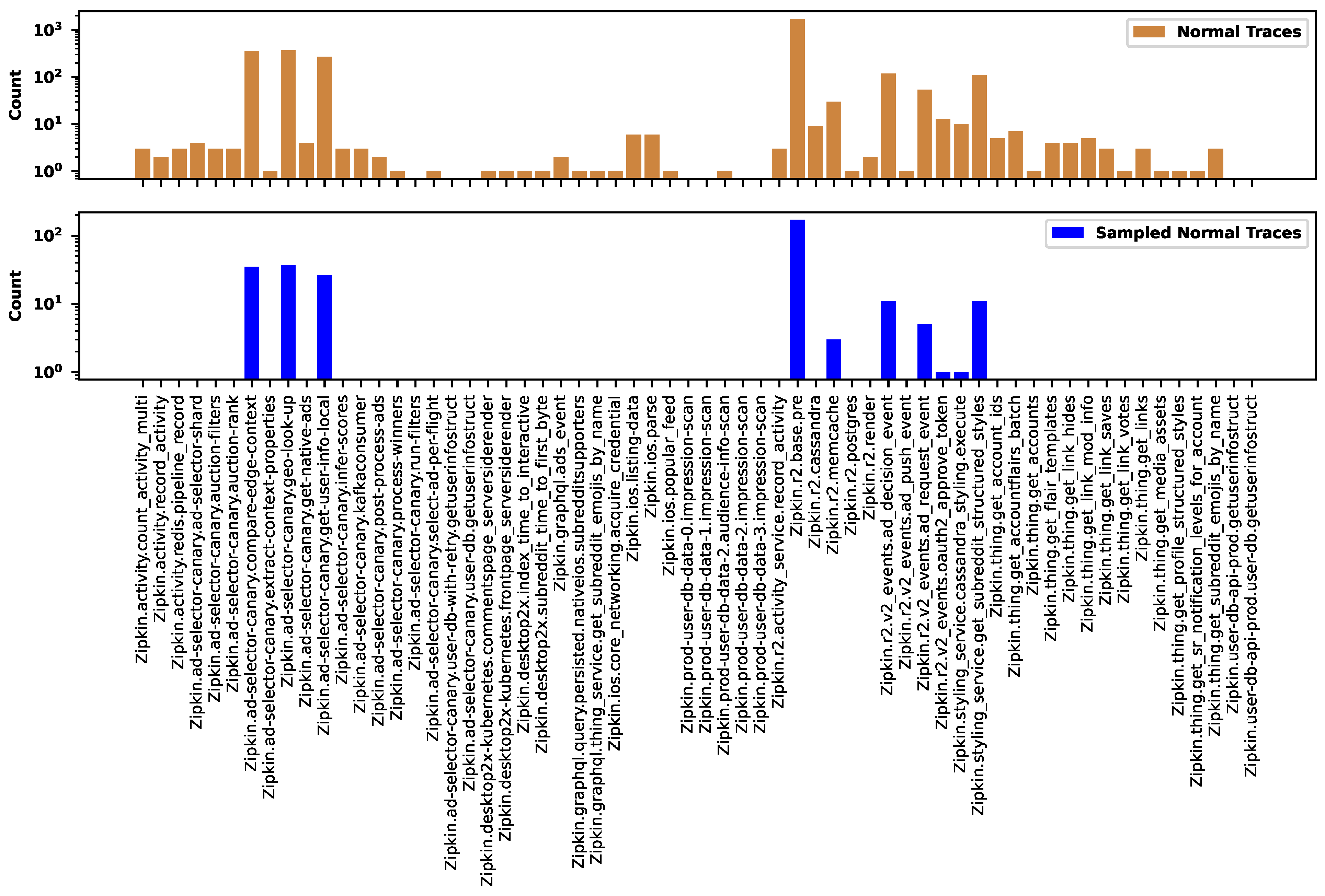
Figure 18 shows the distribution of normal traces across different types before (the top figure) and after (the bottom figure) the sampling. There are many types containing just a single representative. The sampling preserves only the common groups and removes all rare types. Here, we applied
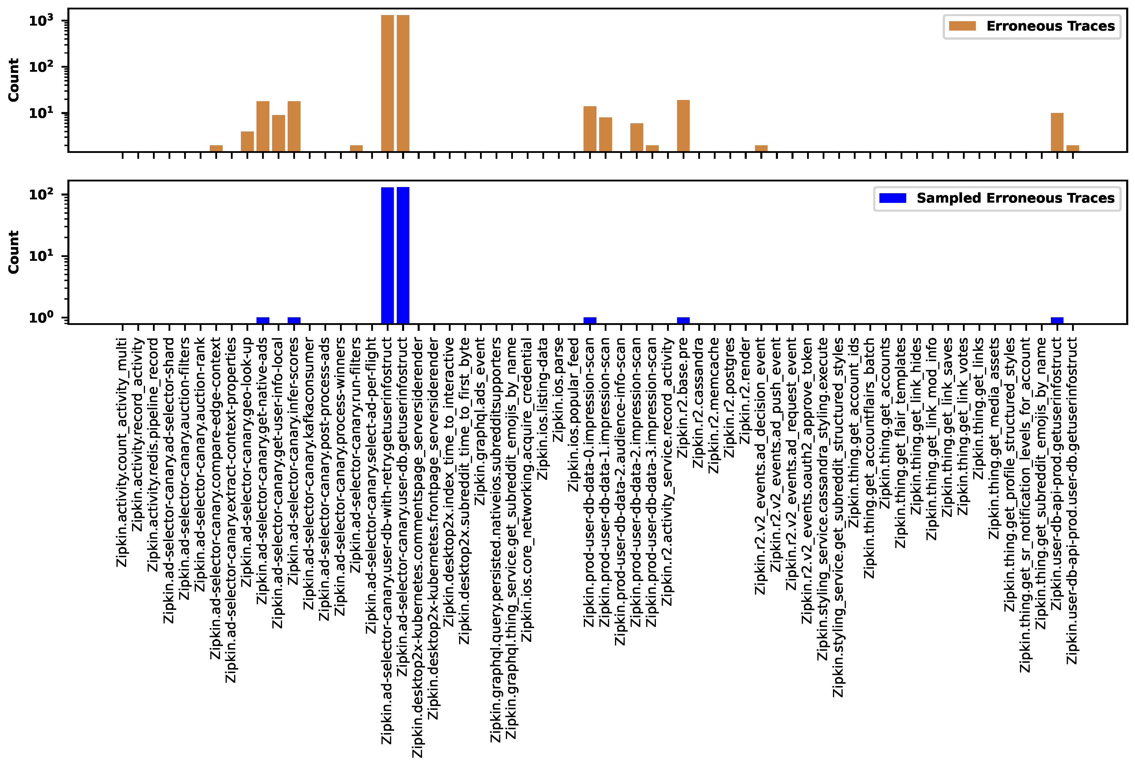
sampling rate. Similarly,
Figure 19 shows the distribution of erroneous traces. In both figures, the labels on the horizontal axes show the names of trace types. We identified the trace type by the root span.
Figure 20 reveals the JRip rules after the sampling, which preserved the first two important rules and removed the others connected with the noise. The sampled dataset contains 300 normal and 268 erroneous traces. The classifier applied to the sampling dataset shows
accuracy. It misclassified 5 traces. The execution time is
seconds. As a result, the sampling reduces the execution time, especially for noisy datasets. Moreover, it shortens the list of top recommendations so that users can focus on the most important ones.
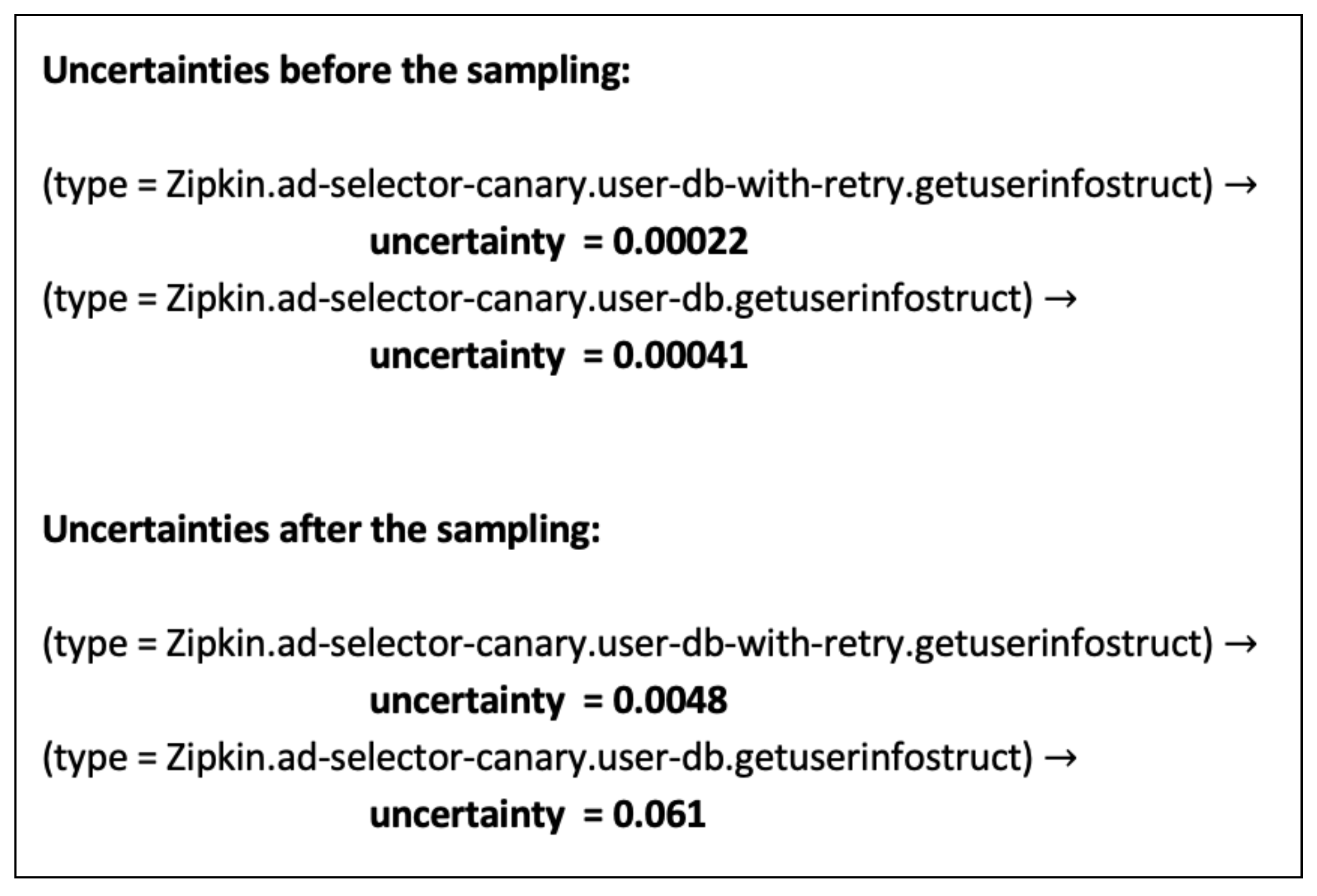
As we mentioned before, the sampling is degrading the statistical evidence. The classifiers cannot describe it. Quite the opposite, the accuracy of classifiers increases or remains almost the same. We can refer to the Dempster-Shafer theory and compare the uncertainties of the rules. The theory of belief functions, also referred to as evidence theory or Dempster–Shafer theory is a general framework for reasoning with uncertainty. It offers an alternative to traditional probabilistic theory for the mathematical representation of uncertainty.
Figure 21 shows how the sampling affects the uncertainties. It shows the uncertainties of the first two rules before and after the sampling.
5. Conclusions
Distributed tracing is essential for gaining visibility into the complex interactions and dependencies within native cloud applications. By tracing the requests across microservices, containers, and dynamic environments, users can effectively monitor, manage, and troubleshoot their cloud-native applications to ensure optimal performance and reliability. Despite the efforts, adopting this technology encounters several challenges, and one of the most crucial is the volume of data and the corresponding resource consumption needed to handle it.
Sampling is a technique that alleviates the overhead of collecting, storing, and processing vast amounts of trace data. It reduces the volume of data by selectively capturing only a fraction of traces. This approach offers benefits such as decreased latency, reduced resource consumption, and improved scalability. However, sampling introduces challenges, particularly in maintaining representative samples and preserving the accuracy of analysis results. Striking a balance between sampling rate and data fidelity is crucial to ensure effective troubleshooting and performance analysis in distributed systems. Overall, distributed tracing sampling plays a vital role in managing the complexity of distributed environments while optimizing resource utilization and maintaining analytical efficacy.
We explored several approaches for sampling that preserved traces with some specific properties. One such property was the type of trace that described the transaction similarity. The traces of the same type normally should have almost the same structure. The goal of such sampling was to preserve traces across all available types. Another property was the duration of the trace. This approach could or might not be combined with the information regarding the type. Trace durations were important as they described the transaction duration. Similar transactions had some typical/ average durations. Atypical durations indicated a transaction/microservice malfunction. The next important trace characteristic was its normality. Erroneous traces carried important information regarding the problems. Hence, it was natural to try to keep all representatives while monitoring the performance of microservices. The flow of erroneous traces would show which microservices had degraded performance. Further, those traces were critical sources of information for troubleshooting application issues.
We sampled only dominant/common errors at the troubleshooting stage, trying to remove the rare ones. This removed the noise and made explanations more confident. The root cause analysis could be performed by tracing traffic passing through a malfunctioning microservice. Rule learning ML methods could help generate explicit rules that explain the problems and clarify the remediation process. We showed how rule-induction systems like RIPPER solved this problem and provided recommendations system administrators could follow to accelerate the resolution process. We also showed that the sampling could dramatically decrease the time of the program execution and provide more clear recommendations. However, as mentioned before, the sampling degraded the statistics, and sometimes rare but important evidence could escape the analysis.
6. Patents
Poghosyan A., Harutyunyan A., Grigoryan N., Pang C., Oganesyan G., Baghdasaryan D., Automated methods and systems that facilitate root-cause analysis of distributed-application operational problems and failures by generating noise-subtracted call-trace-classification rules. Filed: Oct 1, 2021. Application No.: US 17/492,099. Patent No.: US 11880272 B2. Granted: Jan 23, 2024.
Poghosyan A., Harutyunyan A., Grigoryan N., Pang C., Oganesyan G., Baghdasaryan D., Automated methods and systems that facilitate root cause analysis of distributed-application operational problems and failures. Filed: Oct 1, 2021. Application No.: US 17/491,967. Patent No.: US 11880271 B2. Granted: Jan 23, 2024.
Poghosyan, A., Harutyunyan, A., Grigoryan, N., Pang, C., Oganesyan, G., and Avagyan, K., Methods and systems for intelligent sampling of application traces. Application filed by VMware LLC in 2021. Application No.: US 17/367,490. Patent No.: US 11940895 B2. Granted: Mar 26, 2024.
Poghosyan, A.V., Harutyunyan, A.N., Grigoryan, N.M., Pang, C., Oganesyan, G., and Avagyan, K., Methods and systems for intelligent sampling of normal and erroneous application traces. Application filed by VMware LLC in 2021. Application No.: US 17/374,682. Publication of US 20220291982 A1 in 2022.
Poghosyan, A.V., Harutyunyan, A.N., Grigoryan, N.M., N. M., Pang, C., Oganesyan, G., and Baghdasaryan, D., Automated methods and systems that facilitate root cause analysis of distributed-application operational problems and failures. Application filed by VMware LLC in 2021. Application No.: US 17/491,967 and 17/492,099.
Grigoryan N.M., Poghosyan A., Harutyunyan A.N., Pang C., Nag D.A., Methods and Systems that Identify Dimensions Related to Anomalies in System Components of Distributed Computer Systems using Clustered Traces, Metrics, and Component-Associated Attribute Values. Filed: Dec 12, 2020. Application No.: US 17/119,462. Patent No.: US 11,416,364 B2. Granted: Aug 16, 2022.
Author Contributions
Conceptualization, Arnak Poghosyan, Ashot Harutyunyan and Nelson Baloian; Data curation, Edgar Davtyan and Karen Petrosyan; Formal analysis, Arnak Poghosyan and Ashot Harutyunyan; Investigation, Arnak Poghosyan and Ashot Harutyunyan; Methodology, Arnak Poghosyan and Ashot Harutyunyan; Project administration, Nelson Baloian; Resources, Nelson Baloian; Software, Edgar Davtyan and Karen Petrosyan; Supervision, Nelson Baloian; Validation, Arnak Poghosyan and Ashot Harutyunyan; Visualization, Edgar Davtyan and Karen Petrosyan; Writing – original draft, Arnak Poghosyan and Ashot Harutyunyan; Writing – review and editing, Arnak Poghosyan, Ashot Harutyunyan, Edgar Davtyan, Karen Petrosyan and Nelson Baloian.
Funding
This research was funded by ADVANCE Research Grants from the Foundation for Armenian Science and Technology.
Data Availability Statement
Data is confidential. However, we can share data upon request without unveiling the customers and their environments from where the data were taken.
Acknowledgments
The authors are thankful to the anonymous reviewers for very constructive recommendations and comments, which helped improve the presentation of this material.
Conflicts of Interest
The authors declare no conflicts of interest. The funders had no role in the design of the study, in the collection, analyses, or interpretation of data, in the writing of the manuscript, or in the decision to publish the results.
Abbreviations
The following abbreviations are used in this manuscript:
| AI |
Artificial Intelligence |
| AIOps |
AI for IT Operations |
| API |
Application Programming Interface |
| AWS |
Amazon Web Services |
| DST |
Dempster-Shafer Theory |
| IT |
Information Technologies |
| MAD |
Median absolute Deviation |
| ML |
Machine Learning |
| MTTD |
Mean Time to Detect |
| MTTR |
Mean Time to Repair |
| SRE |
Site Reliability Engineer |
| XAI |
Explainable Artificial Intelligence |
References
- Parker, A.; Spoonhower, D.; Mace, J.; Sigelman, B.; Isaacs, R. Distributed Tracing in Practice: Instrumenting, Analyzing, and Debugging Microservices; O’Reilly Media, Incorporated, 2020.
- Shkuro, Y. Mastering Distributed Tracing: Analyzing performance in microservices and complex systems; Packt Publishing, 2019.
- Opentracing. What is distributed tracing? https://opentracing.io/docs/overview/what-is-tracing/, 2019. Accessed: 2021-01-26.
- Cai, Z.; Li, W.; Zhu, W.; Liu, L.; Yang, B. A real-time trace-level toot-cause diagnosis system in Alibaba datacenters. IEEE Access 2019, 7, 142692–142702.
- Liu, D.; He, C.; Peng, X.; Lin, F.; Zhang, C.; Gong, S.; Li, Z.; Ou, J.; Wu, Z. MicroHECL: High-Efficient Root Cause Localization in Large-Scale Microservice Systems. 2021 IEEE/ACM 43rd International Conference on Software Engineering: Software Engineering in Practice (ICSE-SEIP), 2021, pp. 338–347.
- Poghosyan, A.V.; Harutyunyan, A.N.; Grigoryan, N.M.; Pang, C. Root Cause Analysis of Application Performance Degradations via Distributed Tracing. Third CODASSCA Workshop, Yerevan, Armenia: Collaborative Technologies and Data Science in Artificial Intelligence Applications; Hajian, A.; Baloian, N.; Inoue, T.; Luther, W., Eds.; Logos Verlag: Berlin, 2022; pp. 27–31.
- Poghosyan, A.; Harutyunyan, A.; Grigoryan, N.; Pang, C. Distributed Tracing for Troubleshooting of Native Cloud Applications via Rule-Induction Systems. JUCS - Journal of Universal Computer Science 2023, 29, 1274–1297.
- Distributed Tracing - Past, Present and Future.https://www.zerok.ai/post/distributed-tracing-past-present-future, 2023.
- Young, T.; Parker, A. Learning OpenTelemetry; O’Reilly Media, 2024.
- Cotroneo, D.; De Simone, L.; Liguori, P.; Natella, R. Run-time failure detection via non-intrusive event analysis in a large-scale cloud computing platform. Journal of Systems and Software 2023, 198, 111611.
- Zhang, X.; Lin, Q.; Xu, Y.; Qin, S.; Zhang, H.; Qiao, B.; Dang, Y.; Yang, X.; Cheng, Q.; Chintalapati, M.; Wu, Y.; Hsieh, K.; Sui, K.; Meng, X.; Xu, Y.; Zhang, W.; Shen, F.; Zhang, D. Cross-dataset Time Series Anomaly Detection for Cloud Systems. 2019 USENIX Annual Technical Conference (USENIX ATC 19); USENIX Association: Renton, WA, 2019; pp. 1063–1076.
- Poghosyan, A.; Harutyunyan, A.; Grigoryan, N.; Pang, C.; Oganesyan, G.; Ghazaryan, S.; Hovhannisyan, N. An Enterprise Time Series Forecasting System for Cloud Applications Using Transfer Learning. Sensors 2021, 21.
- Abad, C.; Taylor, J.; Sengul, C.; Yurcik, W.; Zhou, Y.; Rowe, K. Log correlation for intrusion detection: A proof of concept. 19th Annual Computer Security Applications Conference, 2003. Proceedings., 2003, pp. 255–264.
- Suriadi, S.; Ouyang, C.; van der Aalst, W.; ter Hofstede, A. Root cause analysis with enriched process logs. Business Process Management Workshops, International Workshop on Business Process Intelligence (BPI 2012). Volume 132 of Lecture Notes in Business Information Processing; Rosa, M.L.; Soffer, P., Eds.; Springer-Verlag: Berlin, 2013; pp. 174–186.
- BigPanda. Incident Management. https://docs.bigpanda.io/docs/incident-management, 2020. Accessed: 2021-01-26.
- Josefsson, T. Root-cause analysis through machine learning in the cloud; Uppsala Universitet, 2017.
- Tak, B.; Tao, S.; Yang, L.; Zhu, C.; Ruan, Y. LOGAN: Problem diagnosis in the cloud using log-based reference models. 2016 IEEE International Conference on Cloud Engineering (IC2E) 2016, pp. 62–67.
- Mi, H.; Wang, H.; Zhou, Y.; Lyu, M.R.; Cai, H. Localizing root causes of performance anomalies in cloud computing systems by analyzing request trace logs. SCIENCE CHINA Information Sciences 2012, 55, 2757–2773.
- Barredo Arrieta, A.; Díaz-Rodríguez, N.; Del Ser, J.; Bennetot, A.; Tabik, S.; Barbado, A.; Garcia, S.; Gil-Lopez, S.; Molina, D.; Benjamins, R.; Chatila, R.; Herrera, F. Explainable Artificial Intelligence (XAI): Concepts, taxonomies, opportunities and challenges toward responsible AI. Information Fusion 2020, 58, 82 – 115.
- Cohen, W.W. Fast Effective Rule Induction. Proceedings of the Twelfth International Conference on Machine Learning. Morgan Kaufmann, 1995, pp. 115–123.
- Quinlan, J.R. C4.5: Programs for machine learning; Elsevier, 2014.
- Las-Casas, P.; Papakerashvili, G.; Anand, V.; Mace, J. Sifter: Scalable Sampling for Distributed Traces, without Feature Engineering. Proceedings of the ACM Symposium on Cloud Computing; Association for Computing Machinery: New York, NY, USA, 2019; SoCC ’19, p. 312–324.
- Thereska, E.; Salmon, B.; Strunk, J.; Wachs, M.; Abd-El-Malek, M.; Lopez, J.; Ganger, G.R. Stardust: Tracking activity in a distributed storage system. Proceedings of Joint International Conference on Measurement and Modeling of Computer Systems (SIGMETRICS’06); ACM, , 2006.
- Sambasivan, R.R.; Zheng, A.X.; Rosa, M.D.; Krevat, E.; Whitman, S.; Stroucken, M.; Wang, W.; Xu, L.; Ganger, G.R. Diagnosing performance changes by comparing request flows. 8th USENIX Symposium on Networked Systems Design and Implementation (NSDI), 2011.
- Fonseca, R.; Porter, G.; Katz, R.H.; Shenker, S.; Stoica, I. X-trace: A pervasive network tracing framework. Proceedings of the 4th USENIX Conference on Networked Systems Design & Implementation; USENIX Association: USA, 2007; NSDI’07, p. 20.
- Sigelman, B.H.; Barroso, L.A.; Burrows, M.; Stephenson, P.; Plakal, M.; Beaver, D.; Jaspan, S.; Shanbhag, C. Dapper, a Large-Scale Distributed Systems Tracing Infrastructure. Technical report, Google, Inc., 2010.
- Kaldor, J.; Mace, J.; Bejda, M.; Gao, E.; Kuropatwa, W.; O’Neill, J.; Ong, K.W.; Schaller, B.; Shan, P.; Viscomi, B.; Venkataraman, V.; Veeraraghavan, K.; Song, Y.J. Canopy: An End-to-End Performance Tracing And Analysis System. Proceedings of the 26th Symposium on Operating Systems Principles; Association for Computing Machinery: New York, NY, USA, 2017; SOSP ’17, p. 34–50.
- OpenTelemetry. https://opentelemetry.io/, 2024.
- Las-Casas, P.; Mace, J.; Guedes, D.; Fonseca, R. Weighted Sampling of Execution Traces: Capturing More Needles and Less Hay. Proceedings of the ACM Symposium on Cloud Computing; Association for Computing Machinery: New York, NY, USA, 2018; SoCC ’18, p. 326–332.
- Google Cloud Observability: Trace Sampling. https://cloud.google.com/trace/docs/trace-sampling, 2024.
- OpenCensus: Sampling. https://opencensus.io/tracing/sampling/ , 2024.
- Azure Monitor: Sampling in Application Insights.https://learn.microsoft.com/en-us/azure/azure-monitor/app/sampling-classic-api, 2024.
- He, S.; Feng, B.; Li, L.; Zhang, X.; Kang, Y.; Lin, Q.; Rajmohan, S.; Zhang, D. STEAM: Observability-Preserving Trace Sampling. FSE’23 Industry, 2023.
- AWS: Advanced Sampling using ADOT.https://aws-otel.github.io/docs/getting-started/advanced-sampling#best-practices-for-advanced-sampling, 2024.
- Jaeger: Sampling. https://www.jaegertracing.io/docs/1.55/sampling/, 2024.
- Anomaly Detection in Zipkin Trace Data.https://engineering.salesforce.com/anomaly-detection-in-zipkin-trace-data-87c8a2ded8a1/, 2024.
- LightStep: Sampling, verbosity, and the case for (much) broader applications of distributed tracing.https://medium.com/lightstephq/sampling-verbosity-and-the-case-for-much-broader-applications-of-distributed-tracing-f3500a174c17, 2024.
- Datadog: Trace Sampling Use Cases.https://docs.datadoghq.com/tracing/guide/ingestion_sampling_use_cases/, 2024.
- Partial trace sampling: A new approach to distributed trace sampling.https://engineering.dynatrace.com/blog/partial-trace-sampling-a-new-approach-to-distributed-trace-sampling/, 2024.
- New Relic: Technical distributed tracing details.https://docs.newrelic.com/docs/distributed-tracing/concepts/how-new-relic-distributed-tracing-works/#sampling, 2024.
- OpenTelemetry Trace Sampling.https://docs.appdynamics.com/observability/cisco-cloud-observability/en/application-performance-monitoring/opentelemetry-trace-sampling, 2024.
- When to Sample. https://docs.honeycomb.io/manage-data-volume/sample/guidelines/, 2024.
- An introduction to trace sampling with Grafana Tempo and Grafana Agent.https://grafana.com/blog/2022/05/11/an-introduction-to-trace-sampling-with-grafana-tempo-and-grafana-agent/, 2024.
- Application Performance Monitoring: Transaction sampling.https://www.elastic.co/guide/en/observability/current/apm-sampling.html, 2024.
- Solé, M.; Muntés-Mulero, V.; Rana, A.I.; Estrada, G. Survey on models and techniques for root-cause analysis. ArXiv:1701.08546, 2017, [arXiv:cs.AI/1701.08546].
- Harutyunyan, A.N.; Poghosyan, A.V.; Grigoryan, N.M.; Hovhannisyan, N.A.; Kushmerick, N. On machine learning approaches for automated log management. J. Univers. Comput. Sci. (JUCS) 2019, 25, 925–945.
- Poghosyan, A.; Ashot, N.; G.M., N.; Kushmerick, N. Incident Management for Explainable and Automated Root Cause Analysis in Cloud Data Centers. JUCS - Journal of Universal Computer Science 2021, 27, 1152–1173.
- Poghosyan, A.V.; Harutyunyan, A.N.; Grigoryan, N.M. Managing cloud infrastructures by a multi-layer data analytics. 2016 IEEE International Conference on Autonomic Computing, ICAC 2016, Wuerzburg, Germany, July 17-22, 2016; Kounev, S.; Giese, H.; Liu, J., Eds. IEEE Computer Society, 2016, pp. 351–356.
- Poghosyan, A.; Harutyunyan, A.; Grigoryan, N.; Pang, C.; Oganesyan, G.; Ghazaryan, S.; Hovhannisyan, N. An Enterprise Time Series Forecasting System for Cloud Applications Using Transfer Learning. Sensors 2021, 21.
- Marvasti, M.A.; Poghosyan, A.V.; Harutyunyan, A.N.; Grigoryan, N.M. Pattern detection in unstructured data: An experience for a virtualized IT infrastructure. 2013 IFIP/IEEE International Symposium on Integrated Network Management, IM 2013, Ghent, Belgium, May 27-31, 2013; Turck, F.D.; Diao, Y.; Hong, C.S.; Medhi, D.; Sadre, R., Eds. IEEE, 2013, pp. 1048–1053.
- Reynolds, P.; Killian, C.E.; Wiener, J.L.; Mogul, J.C.; Shah, M.A.; Vahdat, A. Pip: Detecting the Unexpected in Distributed Systems. Symposium on Networked Systems Design and Implementation, 2006.
- Harutyunyan, A.; Poghosyan, A.; Harutyunyan, L.; Aghajanyan, N.; Bunarjyan, T.; Vinck, A.H. Challenges and Experiences in Designing Interpretable KPI-diagnostics for Cloud Applications. JUCS - Journal of Universal Computer Science 2023, 29, 1298–1318. [CrossRef]
- Harutyunyan, A.N.; Poghosyan, A.V.; Grigoryan, N.M.; Hovhannisyan, N.A.; Kushmerick, N. On Machine Learning Approaches for Automated Log Management. JUCS - Journal of Universal Computer Science 2019, 25, 925–945. [CrossRef]
- Fürnkranz, J.; Gamberger, D.; Lavrač, N. Foundations of rule learning; Cognitive Technologies, Springer, Heidelberg, 2012; pp. xviii+334. With a foreword by Geoffrey I. Webb.
- Fürnkranz, J.; Kliegr, T. A brief overview of rule learning. Rule technologies: Foundations, tools, and applications; Bassiliades, N.; Gottlob, G.; Sadri, F.; Paschke, A.; Roman, D., Eds.; Springer International Publishing: Cham, 2015; pp. 54–69.
- Fürnkranz, J. Pruning Algorithms for Rule Learning. Mach. Learn. 1997, 27, 139–172.
- Fürnkranz, J.; Widmer, G. Incremental reduced error pruning. Proc. 11th International Conference on Machine Learning. Morgan Kaufmann, 1994, pp. 70–77.
- Hühn, J.; Hüllermeier, E. FURIA: An algorithm for unordered fuzzy rule induction. Data Min. Knowl. Discov. 2009, 19, 293–319.
- Lin, F.; Muzumdar, K.; Laptev, N.P.; Curelea, M.V.; Lee, S.; Sankar, S. Fast Dimensional Analysis for Root Cause Investigation in a Large-Scale Service Environment. Proceedings of the ACM on Measurement and Analysis of Computing Systems 2020, 4, 1–23.
- Lee, W.; Stolfo, S.J. Data Mining Approaches for Intrusion Detection. Proceedings of the 7th Conference on USENIX Security Symposium - Volume 7; USENIX Association: USA, 1998; SSYM’98, p. 6.
- Helmer, G.; Wong, J.; Honavar, V.; Miller, L. Intelligent agents for intrusion detection. Proceedings IEEE Information Technology Conference, Syracuse, NY. Springer, 1998, pp. 121–124.
- Helmer, G.; Wong, J.S.; Honavar, V.; Miller, L. Automated discovery of concise predictive rules for intrusion detection. Journal of Systems and Software 2002, 60, 165–175.
- Mannila, H.; Toivonen, H.; Verkamo, A.I. Discovering Frequent Episodes in Sequences Extended Abstract. Proceedings of the First International Conference on Knowledge Discovery and Data Mining. AAAI Press, 1995, KDD’95, p. 210–215.
- Liu, H.; Motoda, H., Perspectives of Feature Selection. In Feature Selection for Knowledge Discovery and Data Mining; Springer US: Boston, MA, 1998; pp. 17–41.
- John, G.H.; Kohavi, R.; Pfleger, K. Irrelevant features and the subset selection problem. Machine Learning: Proceedings of the 11th International Conference. Morgan Kaufmann, 1994, pp. 121–129.
- Agrawal, R.; Imieliński, T.; Swami, A. Mining association rules between sets of items in large databases. Proceedings of the 1993 ACM SIGMOD international conference on Management of data, 1993, pp. 207–216.
- Shafer, G. A Mathematical Theory of Evidence; Princeton University Press: Princeton, 1976.
- Peñafiel, S.; Baloian, N.; Sanson, H.; Pino, J.A. Applying Dempster–Shafer theory for developing a flexible, accurate and interpretable classifier. Expert Syst. Appl. 2020, 148.
- Poghosyan, A.; Harutyunyan, A.; Davtyan, E.; Petrosyan, K.; Baloian, N. A Study on Automated Problem Troubleshooting in Cloud Environments with Rule Induction and Verification. Applied Sciences 2024, 14.
- Leys, C.; Ley, C.; Klein, O.; Bernard, P.; Licata, L. Detecting outliers: Do not use standard deviation around the mean, use absolute deviation around the median. Journal of Experimental Social Psychology 2013, 49, 764–766.
- Dunning, T. The t-digest: Efficient estimates of distributions. Software Impacts 2021, 7, 100049.
- Witten, I.H.; Frank, E.; Hall, M.A.; Pal, C.J. Practical machine learning tools and techniques. Morgan Kaufmann 2005.
Figure 1.
Trace sampling multi-layer design.
Figure 1.
Trace sampling multi-layer design.
Figure 2.
Rule-induction systems are applied for the root cause analysis of the problems, also revealing the potential bottlenecks and recommending optimizations.
Figure 2.
Rule-induction systems are applied for the root cause analysis of the problems, also revealing the potential bottlenecks and recommending optimizations.
Figure 3.
The distribution of traces across different types for a specific application.
Figure 3.
The distribution of traces across different types for a specific application.
Figure 4.
The sampling of traces of
Figure 3 for different values of the parameter
.
Figure 4.
The sampling of traces of
Figure 3 for different values of the parameter
.
Figure 5.
The values of show the final sampling rates for different . The red-cross corresponds to with the final sampling rate (around ).
Figure 5.
The values of show the final sampling rates for different . The red-cross corresponds to with the final sampling rate (around ).
Figure 6.
The distribution of traces with different durations (in milliseconds).
Figure 6.
The distribution of traces with different durations (in milliseconds).
Figure 7.
The sampling of traces of
Figure 6 for different values of the parameter
.
Figure 7.
The sampling of traces of
Figure 6 for different values of the parameter
.
Figure 8.
The values of show the sampling rates for the different parameter values . The red cross corresponds to with the total sampling rate (around ).
Figure 8.
The values of show the sampling rates for the different parameter values . The red cross corresponds to with the total sampling rate (around ).
Figure 12.
The sampling rates corresponding to different values . The red cross corresponds to with .
Figure 12.
The sampling rates corresponding to different values . The red cross corresponds to with .
Figure 13.
The sampling rates that correspond to different values of and .
Figure 13.
The sampling rates that correspond to different values of and .
Figure 14.
The sampling of two trace types without counting the errors.
Figure 14.
The sampling of two trace types without counting the errors.
Figure 15.
The sampling of two trace types also counts the errors.
Figure 15.
The sampling of two trace types also counts the errors.
Figure 16.
The sampling of two trace types with more strict requirements on the percentage of erroneous traces. Now we preserve of normal traces and of erroneous ones. The final sampling rate is .
Figure 16.
The sampling of two trace types with more strict requirements on the percentage of erroneous traces. Now we preserve of normal traces and of erroneous ones. The final sampling rate is .
Figure 17.
JRip rules before the sampling.
Figure 17.
JRip rules before the sampling.
Figure 18.
The distribution of normal traces across the types before and after the sampling.
Figure 18.
The distribution of normal traces across the types before and after the sampling.
Figure 19.
The distribution of erroneous traces across the types before and after the sampling.
Figure 19.
The distribution of erroneous traces across the types before and after the sampling.
Figure 20.
JRip rules after the sampling.
Figure 20.
JRip rules after the sampling.
Figure 21.
The uncertainties of rules before and after the sampling.
Figure 21.
The uncertainties of rules before and after the sampling.
Table 1.
The number of traces before and after the samplings.
Table 1.
The number of traces before and after the samplings.
| Type Index |
Original Numbers |
|
|
|
|
| 1 |
788 |
758 |
634 |
439 |
219 |
| 2 |
3996 |
3215 |
2229 |
1339 |
602 |
| 3 |
3778 |
3080 |
2154 |
1301 |
587 |
| 4 |
2082 |
1870 |
1418 |
906 |
426 |
| 5 |
249 |
246 |
222 |
167 |
89 |
| 6 |
2043 |
1839 |
1397 |
895 |
421 |
| 7 |
142 |
142 |
131 |
101 |
56 |
| 8 |
104 |
104 |
97 |
77 |
43 |
| 9 |
64 |
64 |
61 |
49 |
29 |
| 10 |
621 |
603 |
513 |
362 |
184 |
| 11 |
216 |
214 |
194 |
147 |
79 |
| 12 |
62 |
62 |
59 |
48 |
28 |
| 13 |
241 |
239 |
215 |
162 |
87 |
| 14 |
93 |
93 |
87 |
69 |
39 |
| 15 |
49 |
49 |
47 |
39 |
23 |
| 16 |
44 |
44 |
42 |
35 |
21 |
| 17 |
98 |
98 |
92 |
73 |
41 |
| 18 |
41 |
41 |
40 |
33 |
19 |
| 19 |
3 |
3 |
3 |
3 |
2 |
| 20 |
63 |
63 |
60 |
49 |
28 |
| 21 |
3 |
3 |
3 |
3 |
2 |
| 22 |
3028 |
2580 |
1863 |
1150 |
527 |
| 23 |
1413 |
1316 |
1042 |
689 |
332 |
| 24 |
23 |
23 |
23 |
19 |
12 |
| 25 |
546 |
532 |
457 |
326 |
166 |
| 26 |
58 |
58 |
55 |
45 |
26 |
| 27 |
51 |
51 |
49 |
40 |
23 |
| 28 |
526 |
513 |
442 |
316 |
162 |
| Total |
20425 |
17903 |
13629 |
8882 |
4273 |
| Rate |
- |
87.7% |
66.7% |
43.5% |
20.9% |
Table 2.
The number of traces before and after the samplings.
Table 2.
The number of traces before and after the samplings.
| Time Intervals |
Original Numbers |
|
|
|
|
|
6685 |
4498 |
2861 |
1629 |
707 |
|
5061 |
3808 |
2542 |
1491 |
660 |
|
6328 |
4368 |
2806 |
1607 |
700 |
|
81 |
81 |
76 |
61 |
35 |
|
235 |
233 |
210 |
159 |
85 |
|
1111 |
1051 |
852 |
575 |
281 |
|
925 |
884 |
729 |
499 |
247 |
| Total |
20425 |
14923 |
10076 |
6021 |
2715 |
| Rate |
- |
73.1% |
49.3% |
29.5% |
13.3% |
|
Disclaimer/Publisher’s Note: The statements, opinions and data contained in all publications are solely those of the individual author(s) and contributor(s) and not of MDPI and/or the editor(s). MDPI and/or the editor(s) disclaim responsibility for any injury to people or property resulting from any ideas, methods, instructions or products referred to in the content. |
© 2024 by the authors. Licensee MDPI, Basel, Switzerland. This article is an open access article distributed under the terms and conditions of the Creative Commons Attribution (CC BY) license (http://creativecommons.org/licenses/by/4.0/).
